Multi-Class, Multi-Server Queueing Inventory System with Batch Service

Abstract

In this paper, we consider a queueing inventory system with batch arrival and batch service processes. Customers arrive in batches of sizes $1,2,\dots ,k$, according to a marked compound Poisson process. We call a batch of customers as belonging to j when there are j individual customers in that batch. The service facility has waiting rooms for each category of customers and also a room to serve them. Except for category 1, all other customers have finite waiting rooms. The service room has only a limited number of seats. These seats are arranged in such a fashion that customers belonging to category j have groups of seats, each with j seats for $j=1,2,\dots ,k$. Customers are taken for service according to the availability of seats designated to each category. A category j customer can be taken for service only if j items are available in the inventory. The service time of customers of category j is exponentially distributed with parameter depending on j for $j=1,2,\dots ,k$. The number of seats available in the service room for each category of customers is restricted to a finite number. The replenishment for items follows the $(s,S)$ policy: fill up to S at the time of replenishment. Lead time follows an exponential distribution. We analyze the system in the equilibrium state. Performance characteristics are evaluated and a number of numerical illustrations are provided.

1. Introduction

In real-life applications, customers might arrive in batches of different sizes. Members in each batch are to be served together. Thus, an inventory requirement of a category j batch depends on the number of persons in that batch, which is j. Several researchers studied queueing models with batch arrival and/batch service. Nevertheless, these are without an inventory requirement. In other words, those are pure queueing theoretic problems, whereas the present one is of a queueing-inventory type, which means an inventory with positive service time. These included Niranjan and Indhira [1], Li et al. [2], Jayaramn and Matis [3], Baruah et al. [4], Chen et al. [5], Banerjee et al. [6], Sikdar and Samanta [7] and Al Maqbali et al. [8]. Adan and Resing [9] studied a multi-server batch-service queueing model. In this model, customers arrive one by one according to a Poisson process. These customers are served in batches. However, Chakravarthy and Dudin [10] studied a c-server queueing model and customers arrive according to a batch Markovian arrival process. They are served in groups of different sizes.

Krishnamoorthy and Joshua [11] studied exhaustively a very general batch arrival, batch service single server queue in which successive arriving batch sizes and also successive service batch sizes form two independent Markov chains on two distinct state spaces that are finite. Arrival and service processes were independent batch Markovian (BMAP and BMSP) processes. This was extended in Krishnamoorthy, Joshua, and Kozyrev [12] to study a single server queueing inventory system in which the server utilizes its idle time (arising in distinct ways) to process items (inventory) to be served to the customers. It was assumed that each batch being served needs only one item from the inventory, irrespective of the batch size. However, customers arriving in the same batch were NOT assumed to be served together in that paper.

Zhao and Lian [13] studied a queueing inventory system with two classes of customers. Each service used one item in the attached inventory. Yadavalli et al. [14] studied a queueing inventory system with three different types of customers and two types of items. Al Maqbali et al. [15] studied a queueing inventory system in a transport problem. In their study, they considered the batch arrival of customers to a transport station.

In this paper, we consider a queueing inventory system with batch arrival and batch service. There are k servers, one for each category of customers. Customers arrive in batches of sizes $1,2,\dots ,k$, according to a marked compound Poisson process, with arrival rate $\lambda P_j$, where $P_j$ is the probability that the batch size is j. We label each batch of size j customers as belonging to Type j, meaning that there are j customers in that batch. Type j customers are taken for service only if there is a seat (meaning that seats for j customers belonging to that group) designated to that category and at least j items are available in the inventory. At this point, it is essential to mention that the inventory is counted in units: one item, two items, …, up to the maximum S items, depending on its availability.

Customers are taken for service from the respective queues, designated to each category of customers, according to availability of seats in the service station. Thus, though within a category, the first in first out (FIFO) discipline is applied, for the whole system of customers the FIFO is violated. At this point one may wonder whether the system being analyzed consists of k parallel queues and so why should it not be studied in that form rather than the system as a whole. The fact of the matter is that the inventory is drawn from a common pool. Furthermore, the inventory is not available in abundance. This leads to the dependence of various queues involved. Thus, depending on the availability of vacant seats to each category of customers and also depending on the inventory available, customers are taken for service. The service time of each type j batch is $T_j$, which is exponentially distributed with parameters ${\mu }_j$.

As mentioned in the abstract, there are two distinct types of rooms for each category of customers, the waiting room and the service room for type j, where $j=1,2,\dots ,k$. The waiting room for type j is of finite capacity $W_j$ for $j\ne 1$. However, the waiting room for type 1 is of infinite capacity. The service room for each type is of finite capacity and the maximum number of batches of type j that can be accommodated is $C_j,j=1,2,\dots ,k$.

An inventory of commodities is attached to the service stations as common pool. Each type j requires j units of the items for service, $j=1,2,\dots ,k.$ On being admitted for service, a type j batch takes away j units of inventory. The replenishment for items follows the $(s,S)$ policy: fill up to S at the time of replenishment. The condition imposed on s in terms of $1,2,\dots ,k$ is the following: $\frac{k(k+1)}{2}$; s is chosen so that it is at least as large as r times $\frac{k(k+1)}{2}$, where r is a positive integer. The optimal value of r will be available when we compute that for s. The lead time for replenishment follows an exponential distribution with parameter $\theta .$

Though stated earlier, we wish to stress that there are two conditions, both of which must be satisfied to allow a type j batch to go to the service room. The first condition is that at least j units of inventory are available in store. The second one is that there is enough space in the j-type service room. It is assumed that when inventory for a batch of size b is available and at least one seat for that category is vacant without customers of that type waiting, no other suitable batch of customers is selected for service. This is done to avoid a fractional part of a batch remaining.

If the inventory level reaches s or below for the first time after the previous replenishment, an order is immediately placed to bring the inventory level to S after the random lead time elapses.

If a type 1 customer finds one of these two conditions not satisfied, it must wait in the waiting room for type 1 (infinite capacity) until both conditions are satisfied. For $j=2,\dots ,k,$ a type j arrival can join the system only if the j-type waiting room is not full. Upon joining, it can go to the service station designated for it only if both conditions are satisfied. For example, 100 customers of type 1 in a waiting room for type $1.$ There are no customers of type 1 in the service station and no inventory. Suppose $C_1=9.$ Then, 9 customers of type 1 are transferred to the service station upon replenishment. The system evolves in this fashion.

Though we started this work based on the functioning of a restaurant there are several other areas of application for this model. Cargo loading and unloading may also be modeled as described in this present situation. In restaurants, seats are arranged according to customers arriving in batches of different sizes (subject to a finite maximum quantity). The seat arrangements are depicted in Figure 1 and Figure 2. In case a vacancy for a batch of size b arises in the restaurant with adequate inventory for that batch and no batch size b customers are available, the items cannot be served for a batch of size larger than b. This is because only a fraction of such a batch can be served with the available inventory; further seats for such batches may not be vacant. Furthermore, it leads to redistribution of customers of that batch (of a size larger than b). Customers of the same batch prefer to be served together. However, batches of a size smaller than b can be chosen to be served, provided seats for that category are available and customers of that type are waiting.

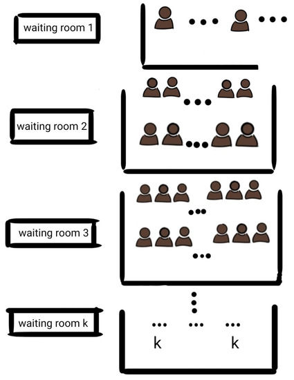
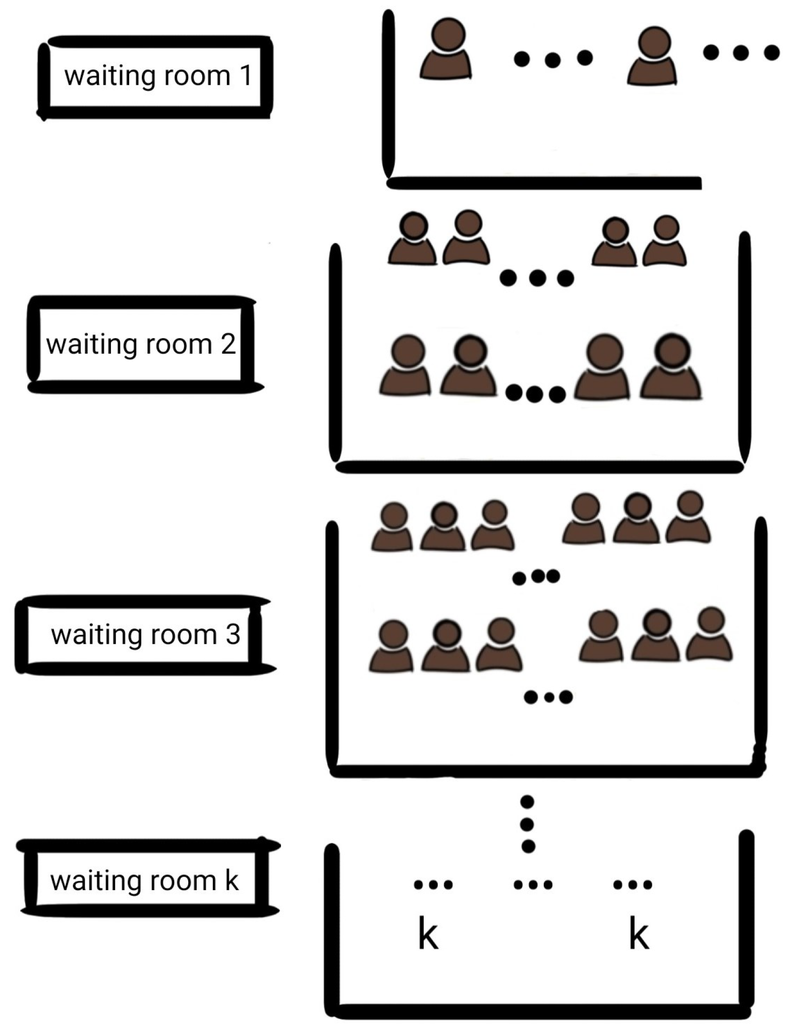
Figure 1. Waiting room for type j where j = 1,2,...,k.

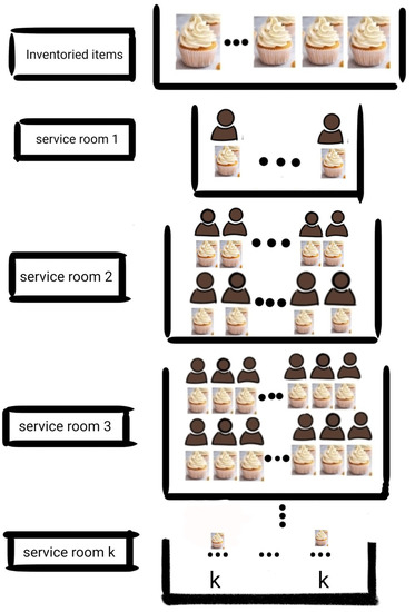
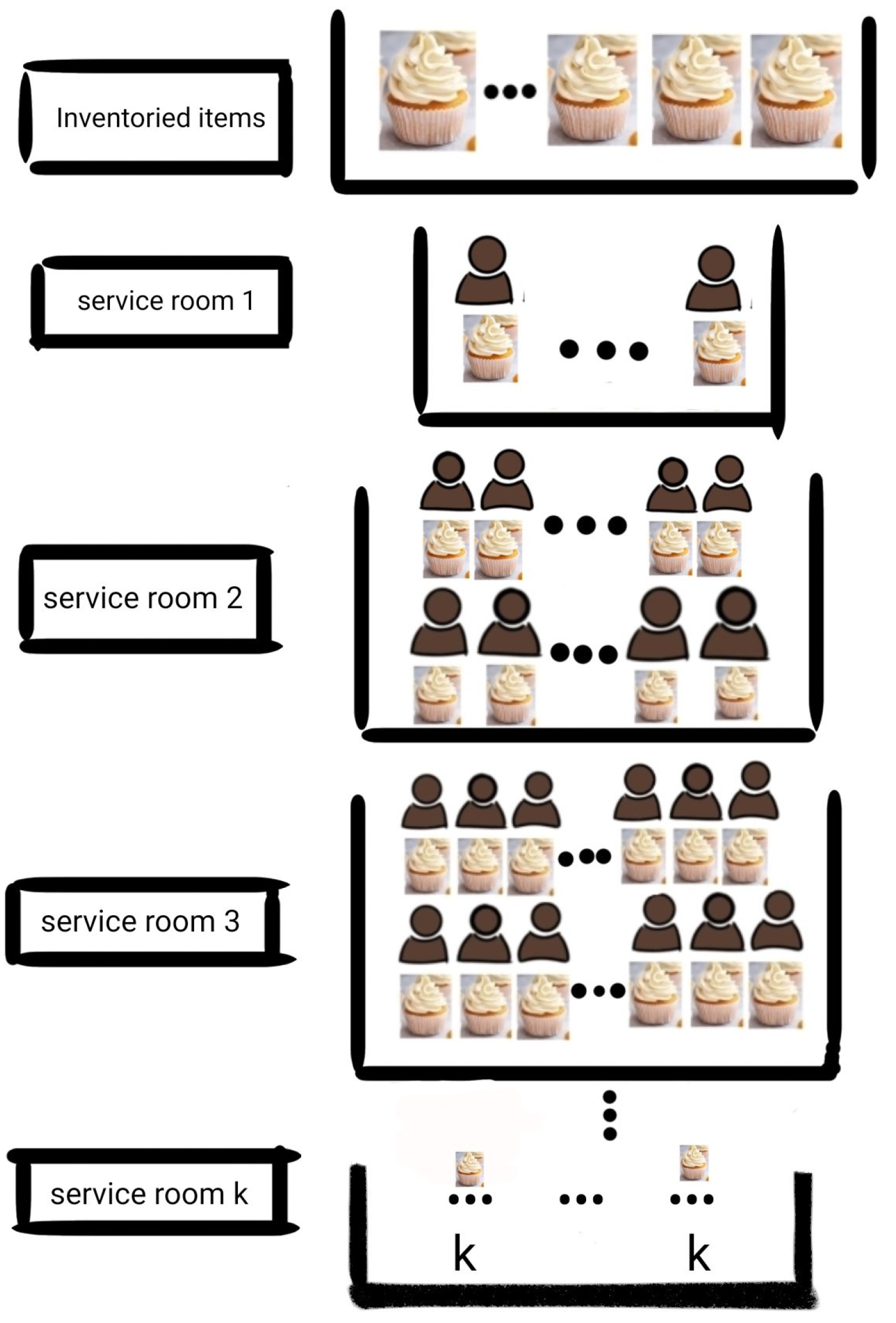
Figure 2. Service room for type j where j = 1,2,...,k.

In theaters seat arrangements are also made, as indicated in the previous example. Nevertheless, a redistribution of seats is made in case groups of a certain size, with seats reserved for the show, do not turn up. In packing of items in boxes this scheme can be adopted to optimally utilize the space while loading into containers.

The salient features of this paper are:

• A multi-class, multi-server queueing-inventory model is discussed for the first time in the literature.
• Arrival of customers forms a marked compound Poisson process.
• Inventory drops down by $1,2,\dots ,k$ units by admitting a batch of size $1,2,\dots ,k$, respectively, for service.
• A very important feature of this model is the drop of type 1 customers in the waiting room: dropping by $1,2,\dots ,C_1$ consequent to a replenishment. This calls for redefining the level to obtain a continuous time Markov chain (CTMC), which is a level-independent quasi-birth-death process (LIQBD).
• In [12], only one item was served to customers belonging to a service batch, irrespective of the number of customers in it. In the present that restriction is removed.

Though the problem discussed in [12] may appear to be more general at a glance, a closer look at the two will reveal that the present work is dealing with a much more complex situation. For example, this paper considers a multi-server problem. Instead of inventory processing by a server, considered in [12], here we consider the purchase of inventory from outside, which is kept in a common pool to serve customers belonging to different types. This is in contrast to [12], where only one item is served to each batch of customers being served, irrespective of the batch size. This is not the case with the problem considered in this paper. Thus, except for the BMAP and BMSP and Markov chain dependence of successive arrival/service batches considered in [12], the present work has many features that are not considered in [12].

The greatest challenge one faces while dealing with this type of modeling is the dimensionality problem. However, this is nothing compared to the information we gain while studying such systems. Further modern computational facilities help in tackling the dimensionality problem to a certain extent.

This paper is arranged as follows. Section 2 discusses the mathematical modeling of the problem under investigation. In Section 3, the stability of the system is investigated and the stationary system state distribution is computed. Performance measures are elaborated in Section 4. In Section 5, the expected cycle length is provided. A cycle is defined as starting from the epoch when inventory on stock drops to s or below for the first time after the previous replenishment, until the next epoch at which the replenishment order is placed. The duration of a chain cycle is referred to as the cycle length. In Section 6, a numerical investigation of the model is elaborated. The optimization problem is elaborated in Section 7. Finally, we finish with a concluding section.

2. Mathematical Description of the Model

We redefine the levels using modulo $C_1.$ This is because when a replenishment takes place, the number of customers of any type in the waiting room can decrease by more than $1.$ This, in particular, results in a decrease by $1,2,\dots ,C_1$ customers of type $1.$

For the analysis of the queueing inventory model, we introduce the following notations:

For $j=1,2,\dots ,k$:

$N_j\left(t\right)$: the number of batches of type j in its waiting room at time t.

$I\left(t\right)$: the number of inventoried items (only the simple type is considered and these are kept in a common pool) at time t.

$M_j\left(t\right)$: the number of batches of type j in its service room at time t.

$X\left(t\right)=\left\{(N_1\left(t\right),N_2\left(t\right),\dots ,N_{k\dots 1}\left(t\right),N_k\left(t\right),I\left(t\right),M_1\left(t\right),M_2\left(t\right),\dots ,M_{k-1}\left(t\right),M_k\left(t\right))\right\}$.

Then, $\left\{X\right(t);t\ge 0\}$ is a continuous time Markov chain on the state space

$\Omega =\left\{(n_1,n_2,\dots ,n_{k-1},n_k,i,m_1,m_2,\dots ,m_{k-1},m_k)\right\}$ with the following restrictions on the possible values:

(I)

If $m_j=C_j$, then $0\le n_j\le W_j; j=2,3,\dots ,k.$

(II)

If $m_1=C_1$, then $n_1\ge 0$.

(III)

$0\le i\le S.$

(IV)

If $i=0$, then $0\le n_1.$

(V)

If $i<j$, then $0\le n_j\le W_j; j=2,3,\dots ,k.$

(VI)

If $i<j$ and $0\le m_j<C_j$, then $0\le n_j\le W_j; j=2,3,\dots ,k.$

(VII)

If $i\ge j$ and $0\le m_j<C_j$, then $n_j=0; j=1,2,\dots ,k.$

(VIII)

If $i=0$ and $0\le m_1<C_1$, then $0\le n_1.$

where $C_j$ is the maximum number of tables size j in a j-type service room for batches of type j where $j=1,2,\dots ,k$, and $W_j$ is the maximum number of tables size j in a j-type waiting room for batches of type j where $j=2,3,\dots ,k$. The waiting rooms and the service rooms are visualized in Figure 1 and Figure 2 below, respectively.

We analyze this model as a level-independent quasi-birth-death (LIQBD) process.

The terms of transitions of the states are given in Table 1, Table 2 and Table 3.

Table 1. Arrival rates.

From	$(0,0,\dots ,0,0,i,m_1,m_2,\dots ,m_{k-1},m_k)$
To	$(0,0,\dots ,0,0,i^{{}^{\prime }},m_1^{{}^{\prime }},m_2^{{}^{\prime }},\dots ,m_{k-1}^{{}^{\prime }},m_k^{{}^{\prime }})$
	$m_j,m_j^{{}^{\prime }}$ where $j=1,2,\dots ,k;$ $0\le i\le S;$
Description	$j\le i$ and $0\le m_j<C_j$
	$i^{{}^{\prime }}=i-j$ and $m_j^{{}^{\prime }}=m_j+1.$
	Only one among $m_1,m_2,\dots ,m_{k-1},m_k$ can be changed with positive probability.
Arrival rate	$\lambda P_j$ where $j=1,2,\dots ,k$
From	$(n_1,n_2,\dots ,n_{k-1},n_k,i,m_1,m_2,\dots ,m_{k-1},m_k)$
To	$(n_1^{{}^{\prime }},n_2^{{}^{\prime }},\dots ,n_{k-1}^{{}^{\prime }},n_k^{{}^{\prime }},i^{{}^{\prime }},m_1^{{}^{\prime }},m_2^{{}^{\prime }},\dots ,m_{k-1}^{{}^{\prime }},m_k^{{}^{\prime }})$
	$n_j,n_j^{{}^{\prime }},m_j,m_j^{{}^{\prime }}$ where $j=1,2,\dots ,k;$
	$0\le i\le S;$
	Subject to one of the following:
	(1) $j\le i$; $n_j=0$; $m_j\ne C_j$; $i^{{}^{\prime }}=i-j$ and $m_j^{{}^{\prime }}=m_j+1$
	(2) $n_j=0$; $m_j=C_j$; $n_j^{{}^{\prime }}=1$ and $i^{{}^{\prime }}=i$
	(3) $0<n_j<W_j$; $m_j=C_j$; $n_j^{{}^{\prime }}=n_j+1$ and $i^{{}^{\prime }}=i.$
Description	(4) $0<n_1$; $m_1=C_1$; $n_1^{{}^{\prime }}=n_1+1$ and $i^{{}^{\prime }}=i.$
	( 5) $j>i$; $0\le n_j<W_j$; $n_j^{{}^{\prime }}=n_j+1$ and $i^{{}^{\prime }}=i.$
	(6) $0\le n_1$; $i=0$; $n_1^{{}^{\prime }}=n_1+1$ and $i^{{}^{\prime }}=0.$
	Only one among $n_1,n_2,\dots ,n_{k-1},n_k,m_1,m_2,\dots ,m_{k-1},m_k$ can be changed with positive probability.
Arrival rate	$\lambda P_j$ where $j=1,2,\dots ,k$

Table 2. Departure rates.

From	$(0,0,\dots ,0,0,i,m_1,m_2,\dots ,m_{k-1},m_k)$
To	$(0,0,\dots ,0,0,i,m_1^{{}^{\prime }},m_2^{{}^{\prime }},\dots ,m_{k-1}^{{}^{\prime }},m_k^{{}^{\prime }})$
	$m_j,m_j^{{}^{\prime }}$ where $j=1,2,\dots ,k;$ $0\le i\le S$
Description	$0<m_j\le C_j$ and $m_j^{{}^{\prime }}=m_j-1$.
	Only one among $m_1,m_2,\dots ,m_{k-1},m_k$ can be changed with positive probability.
Departure rate	${\mu }_j$ where $j=1,2,\dots ,k$.
From	$(n_1,n_2,\dots ,n_{k-1},n_k,i,m_1,m_2,\dots ,m_{k-1},m_k)$
To	$(n_1^{{}^{\prime }},n_2^{{}^{\prime }},\dots ,n_{k-1}^{{}^{\prime }},n_k^{{}^{\prime }},i^{{}^{\prime }},m_1^{{}^{\prime }},m_2^{{}^{\prime }},\dots ,m_{k-1}^{{}^{\prime }},m_k^{{}^{\prime }})$
	$n_j,n_j^{{}^{\prime }},m_j,m_j^{{}^{\prime }}$ where $j=1,2,\dots ,k;$
	Subject to one of the following:
	(1) $1\le n_j\le W_j$; $1\le i\le S$; $j\le i$;
	$m_j=C_j$; $n_j^{{}^{\prime }}=n_j-1$ and $i^{{}^{\prime }}=i-j$;
	where $j=2,3,\dots ,k.$
Description	(2) $1\le n_1$; $1\le i\le S$; $1\le i$; $m_1=C_1$;
	$n_1^{{}^{\prime }}=n_1-1$ and $i^{{}^{\prime }}=i-1$.
	(3) $j>i$; $1\le m_j\le C_j$;
	$m_j^{{}^{\prime }}=m_j-1$; and $i^{{}^{\prime }}=i.$
	(4) $i=0$; $1\le m_1\le C_1$; $m_1^{{}^{\prime }}=m_1-1$; and $i^{{}^{\prime }}=0.$
	Only one among $n_1,n_2,\dots ,n_{k-1},n_k,m_1,m_2,\dots ,m_{k-1},m_k$ can be changed with positive probability.
Departure rate	${\mu }_j$ where $j=1,2,\dots ,k$

Table 3. Replenishment rates.

From	$(0,0,\dots ,0,0,i,m_1,m_2,\dots ,m_{k-1},m_k)$
To	$(0,0,\dots ,0,0,S,m_1,m_2,\dots ,m_{k-1},m_k)$
	$m_j$ where $j=1,2,\dots ,k;$
Description	$0\le i\le s$ and $0\le m_j\le C_j$.
Replenishment rate	$\theta$
From	$(n_1,n_2,\dots ,n_{k-1},n_k,i,C_1,C_2,\dots ,C_{k-1},C_k)$
To	$(n_1,n_2,\dots ,n_{k-1},n_k,S,C_1,C_2,\dots ,C_{k-1},C_k)$
	$n_j$ where $j=1,2,\dots ,k;$ $0\le i\le s$;
Description	$0\le n_1$; $0\le n_j\le W_j$ where $j=2,3,\dots ,k;$
Replenishment rate	$\theta$
From	$(n_1,n_2,\dots ,n_{k-1},n_k,i,m_1,m_2,\dots ,m_{k-1},m_k)$
To	$(n_1^{{}^{\prime }},n_2^{{}^{\prime }},\dots ,n_{k-1}^{{}^{\prime }},n_k^{{}^{\prime }},i^{{}^{\prime }},m_1^{{}^{\prime }},m_2^{{}^{\prime }},\dots ,m_{k-1}^{{}^{\prime }},m_k^{{}^{\prime }})$
	$n_j,n_j^{{}^{\prime }},n_j^{{}^{\prime \prime }},m_j,m_j^{{}^{\prime }}$ where $j=1,2,\dots ,k;$
	$0\le i\le s$.
Description	$0\le m_j<C_j;j=1,2,\dots ,k;$ and
	$1\le n_j\le W_j;j=2,3,\dots ,k$; $1\le n_1;$
	$n_j^{{}^{\prime }}=n_j-n_j^{{}^{\prime \prime }}$ and $m_j^{{}^{\prime }}=m_j+n_j^{{}^{\prime \prime }}$ $\forall j$;
	$0\le n_j^{{}^{\prime }}\le W_j;j=2,3,\dots ,k$; $0\le m_j^{{}^{\prime }}\le C_j;$$0\le n_1^{{}^{\prime }};$
	$i^{{}^{\prime }}=S-{\sum }_{j=1}^{k}j{n}_j^{{}^{\prime \prime }}$.
	Note: If $i\ge j$ and $0<n_1$ or $0<n_j\le W_j$ then $m_j=C_j;j=1,2,\dots ,k.$
Replenishment rate	$\theta$

We have to consider two distinct cases: (i) $C_1>S$ and ($ii$) $C_1<S$. This is required because customers of type 1 waiting when the inventory level is equal to zero could fall into one of the above two categories. Accordingly, when replenishment takes place, either S type 1 customers are transferred to the service station provided that $n_1>S$ (case (i)) or $C_1$ customers are transferred to the service station if $n_1>C_1$. If $n_1<min(C_1,S)$, then all of type 1 are transferred to the service station. There could be transfers of customers of other types also resulting in sub-level changes. We have to be equally concerned about level drops in the customers of type 1 because these drops result in the infinitesimal generator of the process obtaining a structure that is not tridiagonal; it can be non-zero because up to a minimum of $(C_1,S)$ to the left of the diagonal is of the $GI/M/1$ type. This is demonstrated in the following example. Suppose $n_1>max(C_1,S)$ and $S>C_1.$ Then, with $S=50,C_1=15$ and $n_1=60$ we will have 15 non-zero blocks below the diagonal. In what follows we assume that $C_1<S.$ Therefore, we redefine the level using modulo $C_1.$ This leads to the infinitesimal generator of the model in the following form:

$$\begin{array}{c}\hfill Q=\left(\begin{array}{ccccccc}{B}_{00}& B_{01}& & & & & \\ B_{10}& A_1& A_0& & & & \\ & A_2& A_1& A_0& & & \\ & & A_2& A_1& A_0& & \\ & & & \ddots & \ddots & \ddots & \end{array}\right);where\end{array}$$

$$\begin{array}{c}\hfill B_{00}=\left(\begin{array}{ccccc}{E}_{00}& E_{01}& E_{02}& \dots & E_{0(k-1)}\\ E_{10}& E_{11}& E_{12}& \dots & E_{1(k-1)}\\ E_{20}& E_{21}& E_{22}& \dots & E_{2(k-1)}\\ ⋮& ⋮& ⋮& \dots & ⋮\\ E_{(k-1)0}& E_{(k-1)1}& E_{(k-1)2}& \dots & E_{(k-1)(k-1)}\end{array}\right);\end{array}$$

$$\begin{array}{c}\hfill B_{01}=\left(\begin{array}{cccc}{E}_{0k}& O& \dots & O\\ E_{1k}& O& \dots & O\\ E_{2(k-1)}& O& \dots & O\\ ⋮& ⋮& ⋮& ⋮\\ E_{(k-1)k}& O& \dots & O\end{array}\right);\end{array}$$

$$\begin{array}{c}\hfill B_{10}=\left(\begin{array}{ccccc}{E}_{k0}& E_{k1}& E_{k2}& \dots & E_{k(k-1)}\\ E_{(k+1)0}& E_{(k+1)1}& E_{(k+1)2}& \dots & E_{(k+1)(k-1)}\\ E_{(k+2)0}& E_{(k+2)1}& E_{(k+2)2}& \dots & E_{(k+2)(k-1)}\\ ⋮& ⋮& ⋮& \dots \\ E_{(k+C_1-1)0}& E_{(k+C_1-1)1}& E_{(k+C_1-1)2}& \dots & E_{(k+C_1-1)(k-1)}\end{array}\right);\end{array}$$

$$\begin{array}{c}\hfill A_1=\left(\begin{array}{cccccccccc}{H}_1& H_0& O& O& O& O& O& O& \dots & O\\ H_2& H_1& H_0& O& O& O& O& O& \dots & O\\ E_0& H_2& H_1& H_0& O& O& O& O& \dots & O\\ E_1& E_0& H_2& H_1& H_0& O& O& O& \dots & O\\ E_2& E_1& E_0& H_2& H_1& H_0& O& O& \dots & O\\ E_3& E_2& E_1& E_0& H_2& H_1& H_0& O& \dots & O\\ \ddots & \ddots & \ddots & \ddots & \ddots & \ddots & \ddots & \ddots & & ⋮\\ E_{\left(l\right)}& E_{(l-1)}& \dots & E_4& E_3& E_2& E_1& E_0& H_2& H_1\end{array}\right);\end{array}$$

$$\begin{array}{c}\hfill A_0=\left(\begin{array}{cccc}O& O& \dots & O\\ O& O& \dots & O\\ O& O& \dots & O\\ ⋮& ⋮& ⋮& ⋮\\ H_0& O& \dots & O\end{array}\right);\end{array}$$

$$\begin{array}{c}\hfill A_2=\left(\begin{array}{cccccccccc}E& E_{\left(l\right)}& E_{(l-1)}& E_{(l-2)}& E_{(l-3)}& \dots & E_2& E_1& E_0& H_2\\ O& E& E_{\left(l\right)}& E_{(l-1)}& E_{(l-2)}& \dots & E_3& E_2& E_1& E_0\\ O& O& E& E_{\left(l\right)}& E_{(l-1)}& \dots & E_4& E_3& E_2& E_1\\ ⋮& ⋮& & \ddots & \ddots & \ddots & \ddots & \ddots & \ddots & \ddots \\ O& O& O& O& O& O& O& O& O& E\end{array}\right);\end{array}$$

where all sub-matrices (the zero matrices, $E,E_{\left(l\right)},\dots ,E_0$ and $H_0,H_1,H_2$) are square matrices of order $r^{\prime }$ where $r^{\prime }=(C_k+1)(C_{(k-1)}+1)\dots (C_1+1)(W_k+1)(W_{(k-1)}+1)\dots (W_2+1)+(C_k+1)(C_{(k-1)}+1)\dots (C_2+1)(W_k+1)(W_{(k-1)}+1)\dots (W_2+1)+(C_k+1)(C_{(k-1)}+1)\dots (C_2+1)(W_k+1)(W_{(k-1)}+1)\dots (W_3+1)+(C_k+1)(C_{(k-1)}+1)\dots (C_3+1)(W_k+1)(W_{(k-1)}+1)\dots (W_3+1)W_2+(C_k+1)(C_{(k-1)}+1)\dots (C_3+1)(C_2+1)(W_k+1)(W_{(k-1)}+1)\dots (W_4+1)+(C_k+1)(C_{(k-1)}+1)\dots (C_4+1)(W_k+1)(W_{(k-1)}+1)\dots W_3{W}_2+\dots +(C_k+1)(C_{(k-1)}+1)\dots (C_2+1)+\dots +(C_k+1)(C_{(k-1)}+1)\dots (C_3+1)W_2.$

For example, when $k=2,C_1=2,C_2=3,W_2=2$ and $s=3$, we obtain the matrices shown in Appendix A.

3. Steady-State Analysis

3.1. Stability Condition

Theorem 1.

The queueing inventory system generated by Q is stable if and only if:

$${\mathit{\pi }}_{{}_{{\mathit{C}}_{\mathbf{1}}}}\lambda P_1{I}_{\left(r^{\prime }\right)}{\mathit{e}}_{{\mathit{r}}^{\prime }}<\phi$$

where:

$$\phi =\sum _{i=1}^{C_1}{\mathit{\pi }}_{\mathit{i}}E{\mathit{e}}_{{\mathit{r}}^{\prime }}+\sum _{i=1}^{(C_1-1)}{\mathit{\pi }}_{\mathit{i}}{E}_{\left(l\right)}{\mathit{e}}_{{\mathit{r}}^{\prime }}+\sum _{i=1}^{(C_1-2)}{\mathit{\pi }}_{\mathit{i}}{E}_{(l-1)}{\mathit{e}}_{{\mathit{r}}^{\prime }}$$

$$+\dots +\sum _{i=1}^4{\mathit{\pi }}_{\mathit{i}}{E}_2{\mathit{e}}_{{\mathit{r}}^{\prime }}+\sum _{i=1}^3{\mathit{\pi }}_{\mathit{i}}{E}_1{\mathit{e}}_{{\mathit{r}}^{\prime }}+\sum _{i=1}^2{\mathit{\pi }}_{\mathit{i}}{E}_0{\mathit{e}}_{{\mathit{r}}^{\prime }}+{\mathit{\pi }}_{\mathit{1}}{H}_2{\mathit{e}}_{{\mathit{r}}^{\prime }}$$

and $H_0=\lambda P_1{I}_{\left(r^{\prime }\right)}$ where $I_{\left(r^{\prime }\right)}$ is an identity matrix of order $r^{\prime }$ and $\mathit{\pi }$$=({\mathit{\pi }}_{\mathbf{1}},{\mathit{\pi }}_{\mathbf{2}},\dots ,{\mathit{\pi }}_{{\mathit{C}}_{\mathbf{1}}})$ is the stationary vector of A where $A=A_2+A_1+A_0$.${\mathit{\pi }}_{\mathit{i}}$ is a sub-vector of order $1\times r^{\prime }$ where $i=1,2,\dots ,C_1$ and $e_{r^{\prime }}$ is a column vector of dimension $r^{\prime }$ consisting of all 1’s.

Proof. 

Let $A=A_2+A_1+A_0$. We can notice that A is an irreducible matrix. Thus, the stationary vector $\mathit{\pi }$ of A exists such that:

$$\mathit{\pi }A=0$$

$$\mathit{\pi }\mathit{e}=1.$$

The Markov chain with the infinitesimal generator Q of the level-independent quasi-birth-death (LIQBD) is stable if and only if:

$$\mathit{\pi }{A}_0\mathit{e}<\mathit{\pi }{A}_2\mathit{e}.$$

Recall that $A_0$ is a square matrix and $A_0=\left(\begin{array}{cccc}O& O& \dots & O\\ O& O& \dots & O\\ O& O& \dots & O\\ ⋮& ⋮& ⋮& ⋮\\ H_0& O& \dots & O\end{array}\right).$

$$\mathit{\pi }{A}_{0}e=({\mathit{\pi }}_{\mathbf{1}},{\mathit{\pi }}_{\mathbf{2}},{\mathit{\pi }}_{\mathbf{2}},\dots ,{\mathit{\pi }}_{{}_{{\mathit{C}}_{\mathbf{1}}}})A_0\mathit{e};$$

where ${\mathit{\pi }}_{\mathbf{1}},{\mathit{\pi }}_{\mathbf{2}},\dots ,{\mathit{\pi }}_{{}_{{\mathit{C}}_{\mathbf{1}}}}$ are sub-vectors of the order $1\times r^{\prime }.$

$$\begin{array}{cc}\mathit{\pi }{A}_0\mathit{e}& =({\mathit{\pi }}_{{}_{{\mathit{C}}_{\mathbf{1}}}}{H}_0,\mathit{O},\mathit{O},\dots ,\mathit{O})\left(\begin{array}{c}{\mathit{e}}_{{\mathit{r}}^{\prime }}\\ {\mathit{e}}_{{\mathit{r}}^{\prime }}\\ ⋮\\ {\mathit{e}}_{{\mathit{r}}^{\prime }}\end{array}\right);\hfill \\ & ={\mathit{\pi }}_{{}_{{\mathit{C}}_{\mathbf{1}}}}{H}_0{\mathit{e}}_{{\mathit{r}}^{\prime }}={\mathit{\pi }}_{{}_{{\mathit{C}}_{\mathbf{1}}}}\lambda P_1{I}_{\left(r^{\prime }\right)}{\mathit{e}}_{{\mathit{r}}^{\prime }}\hfill \end{array}$$

where $H_0=\lambda P_1{I}_{\left(r^{\prime }\right)}$ and $I_{\left(r^{\prime }\right)}$ are an identity matrix of order $r^{\prime }.$

Recall that $A_2$ is a square matrix and

$$A_2=\left(\begin{array}{cccccccccc}E& E_{\left(l\right)}& E_{(l-1)}& E_{(l-2)}& E_{(l-3)}& \dots & E_2& E_1& E_0& H_2\\ O& E& E_{\left(l\right)}& E_{(l-1)}& E_{(l-2)}& \dots & E_3& E_2& E_1& E_0\\ O& O& E& E_{\left(l\right)}& E_{(l-1)}& \dots & E_4& E_3& E_2& E_1\\ ⋮& ⋮& & \ddots & \ddots & \ddots & \ddots & \ddots & \ddots & \ddots \\ O& O& O& O& O& O& O& O& O& E\end{array}\right).$$

$\mathbf{\pi }{A}_{2}e=({\mathit{\pi }}_{\mathbf{1}},{\mathit{\pi }}_{\mathbf{2}},{\mathit{\pi }}_{\mathbf{2}},\dots ,{\mathit{\pi }}_{{}_{{\mathit{C}}_{\mathbf{1}}}})A_2\mathit{e};$ where ${\mathit{\pi }}_{\mathbf{1}},{\mathit{\pi }}_{\mathbf{2}},\dots ,{\mathit{\pi }}_{{}_{{\mathit{C}}_{\mathbf{1}}}}$ are sub-vectors of order $1\times r^{\prime }.$

$$\begin{array}{cc}\hfill \mathit{\pi }{A}_2\mathit{e}& =({\mathit{\pi }}_{\mathbf{1}}E,({\mathit{\pi }}_{\mathbf{1}}{E}_{\left(l\right)}+{\mathit{\pi }}_{\mathbf{2}}E),({\mathit{\pi }}_{\mathbf{1}}{E}_{(l-1)}+{\mathit{\pi }}_{\mathbf{2}}{E}_{\left(l\right)}+{\mathit{\pi }}_{\mathbf{3}}E),\dots ,({\mathit{\pi }}_{\mathbf{1}}{H}_2+{\mathit{\pi }}_{\mathbf{2}}{E}_0+{\mathit{\pi }}_{\mathbf{3}}{E}_1\hfill \\ & +\dots +{\mathit{\pi }}_{{}_{{\mathit{C}}_{\mathbf{1}}}}E\left)\right)\left(\begin{array}{c}{\mathit{e}}_{{\mathit{r}}^{\prime }}\\ {\mathit{e}}_{{\mathit{r}}^{\prime }}\\ ⋮\\ {\mathit{e}}_{{\mathit{r}}^{\prime }}\end{array}\right);\hfill \\ & ={\mathit{\pi }}_{\mathbf{1}}(E+E_{\left(l\right)}+E_{(l-1)}+\dots +E_2+E_1+E_0+H_2){\mathit{e}}_{{\mathit{r}}^{\prime }}\hfill \\ & +{\mathit{\pi }}_{\mathbf{2}}(E+E_{\left(l\right)}+E_{(l-1)}+\dots +E_2+E_1+E_0){\mathit{e}}_{{\mathit{r}}^{\prime }}\hfill \\ & +{\mathit{\pi }}_{\mathbf{3}}(E+E_{\left(l\right)}+E_{(l-1)}+\dots +E_2+E_1){\mathit{e}}_{{\mathit{r}}^{\prime }}\hfill \\ & +{\mathit{\pi }}_{\mathbf{4}}(E+E_{\left(l\right)}+E_{(l-1)}+\dots +E_2){\mathit{e}}_{{\mathit{r}}^{\prime }}\hfill \\ & +⋮\hfill \\ & +{\mathit{\pi }}_{{}_{({\mathit{C}}_{\mathbf{1}}-\mathbf{1})}}(E+E_{\left(l\right)}){\mathit{e}}_{{\mathit{r}}^{\prime }}\hfill \\ & +{\mathbf{\pi }}_{{}_{{\mathit{C}}_{\mathbf{1}}}}E{\mathit{e}}_{{\mathit{r}}^{\prime }}\hfill \end{array}$$

Then,

$$\mathit{\pi }{A}_2\mathit{e}=\sum _{i=1}^{C_1}{\mathit{\pi }}_{\mathit{i}}E{\mathit{e}}_{{\mathit{r}}^{\prime }}+\sum _{i=1}^{(C_1-1)}{\mathit{\pi }}_{\mathit{i}}{E}_{\left(l\right)}{\mathit{e}}_{{\mathit{r}}^{\prime }}+\sum _{i=1}^{(C_1-2)}{\mathit{\pi }}_{\mathit{i}}{E}_{(l-1)}{\mathit{e}}_{{\mathit{r}}^{\prime }}$$

$$+\dots +\sum _{i=1}^4{\mathit{\pi }}_{\mathit{i}}{E}_2{\mathit{e}}_{{\mathit{r}}^{\prime }}+\sum _{i=1}^3{\mathit{\pi }}_{\mathit{i}}{E}_1{\mathit{e}}_{{\mathit{r}}^{\prime }}+\sum _{i=1}^2{\mathit{\pi }}_{\mathit{i}}{E}_0{\mathit{e}}_{{\mathit{r}}^{\prime }}+{\mathit{\pi }}_{\mathbf{1}}{H}_2{\mathit{e}}_{{\mathit{r}}^{\prime }}=\phi ;$$

Since $\mathit{\pi }{A}_0\mathit{e}={\mathit{\pi }}_{{\mathit{C}}_{\mathbf{1}}}\lambda P_1{I}_{\left(r^{\prime }\right)}{\mathit{e}}_{{\mathit{r}}^{\prime }}$ and $\mathit{\pi }{A}_2\mathit{e}=\phi ,$ then the queueing inventory system is stable if and only if:

$${\mathit{\pi }}_{{}_{{\mathit{C}}_{\mathbf{1}}}}\lambda P_1{I}_{\left(r^{\prime }\right)}{\mathit{e}}_{{\mathit{r}}^{\prime }}<\phi .$$

□

3.2. Stationary Distribution

The stationary distribution of the Markov chain under consideration can obtained by solving the set of Equations (1) and (2).

$$\mathbf{X}Q=0;$$

(1)

$$\mathbf{X}e=1.$$

(2)

Let $\mathbf{X}$ be decomposed with Q as follows:

$\mathbf{X}=({\mathbf{X}}_0,{\mathbf{X}}_1,{\mathbf{X}}_2,\dots ),$ where ${\mathbf{X}}_h=({\mathbf{Y}}_{C_{1}h-C_1+1},{\mathbf{Y}}_{C_{1}h-C_1+2},\dots ,{\mathbf{Y}}_{C_{1}h});h=1,2,\dots$

${\mathbf{X}}_0=({\mathbf{X}}_{0\dots 0},{\mathbf{X}}_{0\dots 1},{\mathbf{X}}_{0\dots 2},\dots ,{\mathbf{X}}_{0\dots C_k},{\mathbf{X}}_{0\dots 1m_k},{\mathbf{X}}_{0\dots 2m_k},{\mathbf{X}}_{0\dots 3m_k},\dots ,{\mathbf{X}}_{0\dots C_{(k-1)}{m}_k},{\mathbf{X}}_{0\dots 1m_{(k-1)}{m}_k},$

${\mathbf{X}}_{0\dots 2m_{(k-1)}{m}_k},{\mathbf{X}}_{0\dots 3m_{(k-1)}{m}_k},\dots ,{\mathbf{X}}_{0\dots C_{(k-2)}{m}_{(k-1)}{m}_k},\dots ,{\mathbf{X}}_{1m_3\dots m_k},{\mathbf{X}}_{2m_3\dots m_k},{\mathbf{X}}_{3m_3\dots m_k},\dots ,$

${\mathbf{X}}_{C_2{m}_3\dots m_k},{\mathbf{X}}_{1m_2\dots m_k},{\mathbf{X}}_{2m_2\dots m_k},{\mathbf{X}}_{3m_2\dots m_k},\dots ,{\mathbf{X}}_{C_1{m}_2\dots m_k});$ where $0\le m_j\le C_j;j=1,2,\dots ,k;$

${\mathbf{X}}_{m_1{m}_2\dots m_k}=({\mathbf{X}}_{0m_1{m}_2\dots m_k},{\mathbf{X}}_{1m_1{m}_2\dots m_k},{\mathbf{X}}_{2m_1{m}_2\dots m_k},\dots ,{\mathbf{X}}_{S{m}_1{m}_2\dots m_k});$

${\mathbf{X}}_{0m_1{m}_2\dots m_k}=({\mathbf{X}}_{n_{k}0m_1{m}_2\dots m_k},{\mathbf{X}}_{n_{(k-1)}{n}_{k}0m_1{m}_2\dots m_k},\dots ,{\mathbf{X}}_{n_2{n}_3\dots n_{k}0m_1{m}_2\dots m_k});$ where $0\le n_j\le W_j$; $j=2,3,\dots ,k;$

${\mathbf{X}}_{i{m}_1{m}_2\dots m_k}=({\mathbf{X}}_{n_{k}i{m}_1{m}_2\dots m_k},{\mathbf{X}}_{n_{(k-1)}{n}_{k}i{m}_1{m}_2\dots m_k},\dots ,{\mathbf{X}}_{0n_2{n}_3\dots n_{k}i{m}_1{m}_2\dots m_k});$ if $0<n_j\le W_j$ and $i\ge j$ then $m_j=C_j$; where $i=1,2,\dots ,S;j=2,3,\dots ,k;$

${\mathbf{Y}}_{n_1}=({\mathbf{Y}}_{n_{1}0\dots 00},{\mathbf{Y}}_{n_{1}0\dots 01},{\mathbf{Y}}_{n_{1}0\dots 02},\dots ,{\mathbf{Y}}_{n_{1}0\dots 0W_k},{\mathbf{Y}}_{n_{1}0\dots 10},{\mathbf{Y}}_{n_{1}0\dots 11},{\mathbf{Y}}_{n_{1}0\dots 12},\dots ,{\mathbf{Y}}_{n_{1}0\dots 1W_k},$

${\mathbf{Y}}_{n_{1}0\dots 20},{\mathbf{Y}}_{n_{1}0\dots 21},{\mathbf{Y}}_{n_{1}0\dots 22},\dots ,{\mathbf{Y}}_{n_{1}0\dots 2W_k},\dots ,{\mathbf{Y}}_{n_{1}0\dots W_{(k-1)}0},{\mathbf{Y}}_{n_{1}0\dots W_{(k-1)}1},{\mathbf{Y}}_{n_{1}0\dots W_{(k-1)}2},\dots ,$

${\mathbf{Y}}_{n_{1}0\dots W_{(k-1)}{W}_k},\dots ,{\mathbf{Y}}_{n_1{W}_2{W}_3\dots W_{(k-1)}{W}_k});$ where $n_1=1,2,\dots$

${\mathbf{Y}}_{n_1{n}_2\dots n_{(k-1)}{n}_k}=({\mathbf{Y}}_{n_1{n}_2\dots n_{(k-1)}{n}_{k}0},{\mathbf{Y}}_{n_1{n}_2\dots n_{(k-1)}{n}_{k}1},{\mathbf{Y}}_{n_1{n}_2\dots n_{(k-1)}{n}_{k}2},\dots ,{\mathbf{Y}}_{n_1{n}_2\dots n_{(k-1)}{n}_{k}S});$

${\mathbf{Y}}_{n_1{n}_2\dots n_{(k-1)}{n}_{k}0}=({\mathbf{Y}}_{n_{1}0\dots 0n_{k}0m_1\dots m_k},{\mathbf{Y}}_{n_{1}0\dots 0n_{(k-1)}{n}_{k}0m_1\dots m_k},\dots ,{\mathbf{Y}}_{n_1{n}_2{n}_3\dots n_{(k-1)}{n}_{k}0m_1\dots m_k});$

${\mathbf{Y}}_{n_1{n}_2\dots n_{(k-1)}{n}_{k}i}=({\mathbf{Y}}_{n_{1}0\dots 0n_{k}i{C}_1\dots m_k},{\mathbf{Y}}_{n_{1}0\dots 0n_{(k-1)}{n}_{k}i{C}_1\dots m_k},\dots ,{\mathbf{Y}}_{n_1{n}_2{n}_3\dots n_{(k-1)}{n}_{k}i{C}_1\dots m_k});$ if $0<n_j\le W_j$ and $i\ge j$ then $m_j=C_j$; where $i=1,2,\dots ,S;j=2,3,\dots ,k.$

From Equation (1), we obtain the following equations:

$${\mathbf{X}}_0{B}_{00}+{\mathbf{X}}_1{B}_{10}=0;$$

(3)

$${\mathbf{X}}_0{B}_{01}+{\mathbf{X}}_1{A}_1+{\mathbf{X}}_2{A}_2=0;$$

(4)

$${\mathbf{X}}_1{A}_0+{\mathbf{X}}_2{A}_1+{\mathbf{X}}_3{A}_2=0;$$

(5)

$${\mathbf{X}}_{j-1}{A}_0+{\mathbf{X}}_j{A}_1+{\mathbf{X}}_{j+1}{A}_2=0forj=2,3,\dots$$

(6)

There exists a matrix R such that:

$${\mathbf{X}}_{\mathbf{2}}={\mathbf{X}}_{\mathbf{1}}R;$$

(7)

$${\mathbf{X}}_{\mathbf{j}}={\mathbf{X}}_{\mathbf{1}}{R}^{j-1}\mathrm{for}j=2,3,\dots$$

(8)

Now, we substitute (8) into (6), and obtain:

$$\begin{array}{ccc}\hfill {\mathbf{X}}_1{R}^{j-2}{A}_0+{\mathbf{X}}_1{R}^{j-1}{A}_1+{\mathbf{X}}_1{R}^j{A}_2& =& \hfill 0;\hfill \\ \hfill {\mathbf{X}}_1{R}^{j-2}(A_0+R{A}_1+R^2{A}_2)& =& \hfill 0;\hfill \end{array}$$

Hence,

$$A_0+R{A}_1+R^2{A}_2=0.$$

(9)

To find R from Equation (9), we multiply Equation (9) by $A_1^{-1}$ from the right side as follows: $A_0{A}_1^{-1}+R{A}_1{A}_1^{-1}+R^2{A}_2{A}_1^{-1}=0;$ so $R=-A_0{A}_1^{-1}-R^2{A}_2{A}_1^{-1}.$

By using successive substitution until $R_k$ is closed to $R_{k+1}$, we can find R as follows:

$$\begin{array}{cc}\hfill R_0& \hfill = 0;\hfill \\ \hfill R_{(k+1)}& =& \hfill -A_0{A}_1^{-1}-R_{\left(k\right)}^2{A}_2{A}_1^{-1};\hfill \end{array}$$

If the matrix $A=A_0+A_1+A_2$ is irreducible, then the spectral radius $\rho \left(R\right)$ is less than 1 if and only if $\pi A_{0}e<\pi A_{2}e$, where $\pi$ is the stationary probability vector of matrix $A.$ To find ${\mathbf{X}}_0$ and ${\mathbf{X}}_1$, we substitute Equation (7) into (4), and then we obtain:

$$\begin{array}{ccc}\hfill {\mathbf{X}}_0{B}_{01}+{\mathbf{X}}_1{A}_1+{\mathbf{X}}_{\mathbf{1}}R{A}_2& =& \hfill 0;\hfill \\ \hfill {\mathbf{X}}_0{B}_{01}+{\mathbf{X}}_1(A_1+R{A}_2)& =& \hfill 0.\hfill \end{array}$$

Now, we can rewrite the set of equations

$$\begin{array}{ccc}\hfill {\mathbf{X}}_0{B}_{00}+{\mathbf{X}}_1{B}_{10}& =& \hfill 0;\hfill \\ \hfill {\mathbf{X}}_0{B}_{01}+{\mathbf{X}}_1(A_1+R{A}_2)& =& \hfill 0.\hfill \end{array}$$

as follows:

$$\begin{array}{cccc}\left(\begin{array}{cc}{\mathbf{X}}_0& {\mathbf{X}}_1\end{array}\right)& \left(\begin{array}{cc}{\mathbf{B}}_{00}& {\mathbf{B}}_{01}\\ {\mathbf{B}}_{10}& (A_1+R{A}_2)\end{array}\right)& =& \left(\begin{array}{cc}0& 0\end{array}\right).\end{array}$$

(10)

We can rewrite $\mathbf{X}e=1$ as $({\mathbf{X}}_{\mathbf{0}},{\mathbf{X}}_{\mathbf{1}},{\mathbf{X}}_{\mathbf{2}},\dots )\mathbf{e}=1.$

Thus, ${\mathbf{X}}_{\mathbf{0}}e+{\mathbf{X}}_{\mathbf{1}}e+{\mathbf{X}}_{\mathbf{2}}e+\dots =1$ and

$${\mathbf{X}}_{\mathbf{0}}e+{\mathbf{X}}_{\mathbf{1}}e+\sum _{i=2}^{\infty }{\mathbf{X}}_{\mathbf{i}}e=1.$$

(11)

Now, we substitute Equation (8) into (11), and we obtain:

$$\begin{array}{ccc}\hfill {\mathbf{X}}_{\mathbf{0}}e+{\mathbf{X}}_{\mathbf{1}}e+\sum _{j=2}^{\infty }{\mathbf{X}}_{\mathbf{1}}{R}^{j-1}e& =& \hfill 1;\hfill \\ \hfill {\mathbf{X}}_{\mathbf{0}}e+\sum _{j=1}^{\infty }{\mathbf{X}}_{\mathbf{1}}{R}^{j-1}e& =& \hfill 1.\hfill \end{array}$$

Hence,

$${\mathbf{X}}_{\mathbf{0}}e+\sum _{j=0}^{\infty }{\mathbf{X}}_{\mathbf{1}}{R}^{j}e=1.$$

(12)

Since

$$\sum _{j=0}^{\infty }{R}^j={(I-R)}^{-1};$$

(13)

we substitute (13) into (12), and we obtain:

$${\mathbf{X}}_{\mathbf{0}}e+{\mathbf{X}}_{\mathbf{1}}{(I-R)}^{-1}e=1;(\mathrm{with}\mathrm{normalization}\mathrm{condition}).$$

(14)

Thus, the finite system of Equations (10) and (14) has a unique positive solution for ${\mathbf{X}}_{\mathbf{0}}$ and ${\mathbf{X}}_{\mathbf{1}}.$ Now, we can use Formula 8 to find the stationary probability vector ${\mathbf{X}}_2,{\mathbf{X}}_3,\dots .$ ${\mathbf{X}}_j={\mathbf{X}}_1{R}^{(j-1)}for j=2,3,\dots$ For more details, see Stewart [16].

4. Performance Measures

We obtained some performance measures of the system under steady state as follows:

I.

Expected number of type 1 customers in waiting room 1:

$$E\left[N_1\right]=\sum _{n_1=1}^{\infty }{n}_1{\mathbf{Y}}_{n_1}e.$$

II.

Expected number of type j customers in waiting room j for $j=2,3,\dots ,k$:

$$E\left[N_j\right]=\sum _{n_j=1}^{W_j}\sum _{n_{(j+1)}=1}^{W_{(j+1)}}\dots \sum _{n_k=1}^{W_k}\sum _{m_1=0}^{C_1}\dots \sum _{m_k=0}^{C_k}{n}_j{\mathbf{x}}_{n_j{n}_{(j+1)}\dots n_{k}0m_1\dots m_k}e$$

$$+\sum _{n_{(j-1)}=1}^{W_{(j-1)}}\sum _{n_j=1}^{W_j}\dots \sum _{n_k=1}^{W_k}\sum _{m_1=0}^{C_1}\dots \sum _{m_k=0}^{C_k}{n}_j{\mathbf{x}}_{n_{(j-1)}{n}_j\dots n_{k}0m_1\dots m_k}e$$

$$+\dots +\sum _{n_2=1}^{W_2}\dots \sum _{n_j=1}^{W_j}\dots \sum _{n_k=1}^{W_k}\sum _{m_1=0}^{C_1}\dots \sum _{m_k=0}^{C_k}{n}_j{\mathbf{x}}_{n_2\dots n_j\dots n_{k}0m_1\dots m_k}e$$

$$+\sum _{n_j=1}^{W_j}\sum _{n_{(j+1)}=1}^{W_{(j+1)}}\dots \sum _{n_k=1}^{W_k}\sum _{i=1}^S\sum _{m_1=0}^{C_1}\dots \sum _{m_k=0}^{C_k}{n}_j{\mathbf{x}}_{n_j{n}_{(j+1)}\dots n_{k}i{m}_1\dots m_k}e$$

$$+\sum _{n_{(j-1)}=1}^{W_{(j-1)}}\sum _{n_j=0}^{W_j}\dots \sum _{n_k=0}^{W_k}\sum _{i=1}^S\sum _{m_1=0}^{C_1}\dots \sum _{m_k=0}^{C_k}{n}_j{\mathbf{x}}_{n_{(j-1)}{n}_j\dots n_{k}i{m}_1\dots m_k}e+\dots$$

$$+\sum _{n_2=1}^{W_2}\dots \sum _{n_j=0}^{W_j}\dots \sum _{n_k=0}^{W_k}\sum _{i=1}^S\sum _{m_1=0}^{C_1}\dots \sum _{m_k=0}^{C_k}{n}_j{\mathbf{x}}_{n_2\dots n_j\dots n_{k}i{m}_1\dots m_k}e$$

$$+\sum _{n_1=1}^{\infty }\sum _{n_j=0}^{W_j}\sum _{n_{(j+1)}=0}^{W_{(j+1)}}\dots \sum _{n_k=0}^{W_k}\sum _{m_1=0}^{C_1}\dots \sum _{m_k=0}^{C_k}{n}_j{\mathbf{Y}}_{n_{1}0\dots n_j{n}_{(j+1)}\dots n_{k}0m_1\dots m_k}e$$

$$+\sum _{n_1=1}^{\infty }\sum _{n_{(j-1)}=1}^{W_{(j-1)}}\sum _{n_j=0}^{W_j}\dots \sum _{n_k=0}^{W_k}\sum _{m_1=0}^{C_1}\dots \sum _{m_k=0}^{C_k}{n}_j{\mathbf{Y}}_{n_{1}0\dots n_{(j-1)}{n}_j\dots n_{k}0m_1\dots m_k}e$$

$$+\dots +\sum _{n_1=1}^{\infty }\sum _{n_2=1}^{W_2}\dots \sum _{n_j=0}^{W_j}\dots \sum _{n_k=0}^{W_k}\sum _{m_1=0}^{C_1}\dots \sum _{m_k=0}^{C_k}{n}_j{\mathbf{Y}}_{n_1{n}_2\dots n_j\dots n_{k}0m_1\dots m_k}e$$

$$+\sum _{n_1=1}^{\infty }\sum _{n_j=1}^{W_j}\sum _{n_{(j+1)}=0}^{W_{(j+1)}}\dots \sum _{n_k=0}^{W_k}\sum _{i=1}^S\sum _{m_2=0}^{C_2}\dots \sum _{m_k=0}^{C_k}{n}_j{\mathbf{Y}}_{n_{1}0\dots n_j{n}_{(j+1)}\dots n_{k}i{C}_1\dots m_k}e$$

$$+\sum _{n_1=1}^{\infty }\sum _{n_{(j-1)}=1}^{W_{(j-1)}}\sum _{n_j=1}^{W_j}\dots \sum _{n_k=0}^{W_k}\sum _{i=1}^S\sum _{m_2=0}^{C_1}\dots \sum _{m_k=0}^{C_k}{n}_j{\mathbf{Y}}_{n_{1}0\dots n_{(j-1)}{n}_j\dots n_{k}i{C}_1{m}_2\dots m_k}e$$

$$+\dots +\sum _{n_1=1}^{\infty }\sum _{n_2=1}^{W_2}\dots \sum _{n_j=0}^{W_j}\dots \sum _{n_k=0}^{W_k}\sum _{i=1}^S\sum _{m_2=0}^{C_2}\dots \sum _{m_k=0}^{C_k}{n}_j{\mathbf{Y}}_{n_1{n}_2{n}_3\dots n_j\dots n_{k}i{C}_1{m}_2\dots m_k}e$$

III.

Expected number of items in inventory:

$$E\left[I\right]=\sum _{i=0}^S\sum _{m_1=0}^{C_1}\dots \sum _{m_k=0}^{C_k}i{\mathbf{X}}_{i{m}_1\dots m_k}e+\sum _{n_1=1}^{\infty }\sum _{n_k=0}^{W_k}\sum _{i=1}^S\sum _{m_2=0}^{C_2}\dots \sum _{m_k=0}^{C_k}i{\mathbf{Y}}_{n_{1}00\dots 0n_{k}i{C}_1{m}_2\dots m_k}e$$

$$+\sum _{n_1=1}^{\infty }\sum _{n_{(k-1)}=0}^{W_{(k-1)}}\sum _{n_k=0}^{W_k}\sum _{i=1}^S\sum _{m_2=0}^{C_2}\dots \sum _{m_k=0}^{C_k}i{\mathbf{Y}}_{n_{1}00\dots 0n_{(k-1)}{n}_{k}i{C}_1{m}_2\dots m_k}e+\dots$$

$$+\sum _{n_1=1}^{\infty }\sum _{n_2=1}^{W_2}\dots \sum _{n_{(k-1)}=0}^{W_{(k-1)}}\sum _{n_k=0}^{W_k}\sum _{i=1}^S\sum _{m_2=0}^{C_2}\dots \sum _{m_k=0}^{C_k}i{\mathbf{Y}}_{n_1{n}_2\dots n_{(k-1)}{n}_{k}i{C}_1{m}_2\dots m_k}e$$

IV.

Expected number of type 1 customers in waiting room 1 due to lack of inventory:

$$E\left[I_1\right]=\sum _{n_1=1}^{\infty }\sum _{n_k=0}^{W_k}\sum _{m_1=0}^{C_1}\dots \sum _{m_k=0}^{C_k}{n}_1{\mathbf{Y}}_{n_{1}00\dots 0n_{k}0m_1\dots m_k}e$$

$$+\sum _{n_1=1}^{\infty }\sum _{n_{(k-1)}=0}^{W_{(k-1)}}\sum _{n_k=0}^{W_k}\sum _{m_1=0}^{C_1}\dots \sum _{m_k=0}^{C_k}{n}_1{\mathbf{Y}}_{n_{1}00\dots 0n_{(k-1)}{n}_{k}0m_1\dots m_k}e+\dots$$

$$+\sum _{n_1=1}^{\infty }\sum _{n_2=1}^{W_2}\dots \sum _{n_k=0}^{W_k}\sum _{m_1=0}^{C_1}\dots \sum _{m_k=0}^{C_k}{n}_1{\mathbf{Y}}_{n_1{n}_2\dots n_{(k-1)}{n}_{k}0m_1\dots m_k}e$$

V.

Expected number of type j customers in waiting room j due to lack of inventory for $j=2,3,\dots ,k$:

$$E\left[I_j\right]=\sum _{n_j=1}^{W_j}\sum _{n_{(j+1)}=0}^{W_{(j+1)}}\dots \sum _{n_k=0}^{W_k}\sum _{m_1=0}^{C_1}\dots \sum _{m_k=0}^{C_k}{n}_j{\mathbf{X}}_{n_j{n}_{(j+1)}\dots n_{k}0m_1\dots m_k}e$$

$$+\sum _{n_{(j-1)}=1}^{W_{(j-1)}}\sum _{n_j=0}^{W_j}\dots \sum _{n_k=0}^{W_k}\sum _{m_1=0}^{C_1}\dots \sum _{m_k=0}^{C_k}{n}_j{\mathbf{X}}_{n_{(j-1)}{n}_j\dots n_{k}0m_1\dots m_k}e$$

$$+\dots +\sum _{n_2=1}^{W_2}\dots \sum _{n_j=0}^{W_j}\dots \sum _{n_k=0}^{W_k}\sum _{m_1=0}^{C_1}\dots \sum _{m_k=0}^{C_k}{n}_j{\mathbf{X}}_{n_2\dots n_j\dots n_{k}0m_1\dots m_k}e$$

$$+\sum _{n_j=1}^{W_j}\sum _{n_{(j+1)}=0}^{W_{(j+1)}}\dots \sum _{n_k=0}^{W_k}\sum _{i=1}^{(j-1)}\sum _{m_1=0}^{C_1}\dots \sum _{m_k=0}^{C_k}{n}_j{\mathbf{X}}_{n_j\dots n_{k}i{m}_1\dots m_k}e$$

$$+\sum _{n_{(j-1)}=1}^{W_{(j-1)}}\sum _{n_j=0}^{W_j}\dots \sum _{n_k=0}^{W_k}\sum _{i=1}^{(j-1)}\sum _{m_1=0}^{C_1}\dots \sum _{m_k=0}^{C_k}{n}_j{\mathbf{X}}_{n_{(j-1)}{n}_j\dots n_{k}i{m}_1\dots m_k}e$$

$$+\dots +\sum _{n_2=1}^{W_2}\dots \sum _{n_j=0}^{W_j}\dots \sum _{n_k=0}^{W_k}\sum _{i=1}^{(j-1)}\sum _{m_1=0}^{C_1}\dots \sum _{m_k=0}^{C_k}{n}_j{\mathbf{X}}_{n_{2}0\dots n_j\dots n_{k}i{m}_1\dots m_k}e$$

$$+\sum _{n_1=1}^{\infty }\sum _{n_j=0}^{W_j}\sum _{n_{(j+1)}=0}^{W_{(j+1)}}\dots \sum _{n_k=0}^{W_k}\sum _{m_1=0}^{C_1}\dots \sum _{m_k=0}^{C_k}{n}_j{\mathbf{Y}}_{n_{1}0\dots n_j\dots n_{k}0m_1\dots m_k}e$$

$$+\sum _{n_1=1}^{\infty }\sum _{n_{(j-1)}=1}^{W_{(j-1)}}\sum _{n_j=0}^{W_j}\dots \sum _{n_k=0}^{W_k}\sum _{m_1=0}^{C_1}\dots \sum _{m_k=0}^{C_k}{n}_j{\mathbf{Y}}_{n_{1}0\dots 0n_{(j-1)}{n}_j\dots n_{k}0m_1\dots m_k}e+\dots$$

$$+\sum _{n_1=1}^{\infty }\sum _{n_2=1}^{W_2}\dots \sum _{n_j=0}^{W_j}\dots \sum _{n_k=0}^{W_k}\sum _{m_1=0}^{C_1}\dots \sum _{m_k=0}^{C_k}{n}_j{\mathbf{Y}}_{n_1{n}_2\dots n_j\dots n_{k}0m_1\dots m_k}e$$

$$+\sum _{n_1=1}^{\infty }\sum _{n_j=1}^{W_j}\dots \sum _{n_k=0}^{W_k}\sum _{i=1}^{(j-1)}\sum _{m_2=0}^{C_2}\dots \sum _{m_k=0}^{C_k}{n}_j{\mathbf{Y}}_{n_{1}0\dots n_j\dots n_{k}i{C}_1{m}_2\dots m_k}e$$

$$+\sum _{n_1=1}^{\infty }\sum _{n_{(j-1)}=1}^{W_{(j-1)}}\sum _{n_j=0}^{W_j}\dots \sum _{n_k=0}^{W_k}\sum _{i=1}^{(k-1)}\sum _{m_2=0}^{C_2}\dots \sum _{m_k=0}^{C_k}{n}_j{\mathbf{Y}}_{n_{1}0\dots 0n_{(j-1)}{n}_j\dots n_{k}i{C}_1{m}_2\dots m_k}e+\dots$$

$$+\sum _{n_1=1}^{\infty }\sum _{n_2=1}^{W_2}\sum _{n_3=0}^{W_3}\dots \sum _{n_j=0}^{W_j}\dots \sum _{n_k=0}^{W_k}\sum _{i=1}^{(j-1)}\sum _{m_2=0}^{C_2}\dots \sum _{m_k=0}^{C_k}{n}_j{\mathbf{Y}}_{n_1{n}_2\dots n_j\dots n_{k}i{C}_1{m}_2\dots m_k}e$$

VI.

Probability that server 1 is idle:

$$b_0^1=\sum _{i=0}^S\sum _{m_2=0}^{C_2}\dots \sum _{m_k=0}^{C_k}{\mathbf{X}}_{i0m_2{m}_3\dots m_k}e+\sum _{n_k=1}^{W_k}\sum _{i=0}^S\sum _{m_2=0}^{C_2}\dots \sum _{m_k=0}^{C_k}{\mathbf{X}}_{n_{k}i0m_2\dots m_k}e$$

$$+\sum _{n_{(k-1)}=1}^{W_{(k-1)}}\sum _{n_k=1}^{W_k}\sum _{i=0}^S\sum _{m_2=0}^{C_2}\dots \sum _{m_k=0}^{C_k}{\mathbf{X}}_{n_{(k-1)}{n}_{k}i0m_2\dots m_k}e+\dots$$

$$+\sum _{n_2=1}^{W_2}\sum _{n_3=1}^{W_3}\dots \sum _{n_{(k-1)}=1}^{W_{(k-1)}}\sum _{n_k=1}^{W_k}\sum _{i=0}^S\sum _{m_2=0}^{C_2}\dots \sum _{m_k=0}^{C_k}{\mathbf{X}}_{n_2{n}_3\dots n_{(k-1)}{n}_{k}i0m_2\dots m_k}e$$

$$+\sum _{n_1=1}^{\infty }\sum _{n_k=0}^{W_k}\sum _{m_2=0}^{C_2}\dots \sum _{m_k=0}^{C_k}{\mathbf{Y}}_{n_{1}0\dots 0n_{k}00m_2\dots m_k}e$$

$$+\sum _{n_1=1}^{\infty }\sum _{n_{(k-1)}=1}^{W_{(k-1)}}\sum _{n_k=0}^{W_k}\sum _{m_2=0}^{C_2}\dots \sum _{m_k=0}^{C_k}{\mathbf{Y}}_{n_{1}0\dots 0n_{(k-1)}{n}_{k}00m_2\dots m_k}e+\dots$$

$$+\sum _{n_1=1}^{\infty }\sum _{n_2=1}^{W_2}\sum _{n_3=0}^{W_3}\dots \sum _{n_{(k-1)}=1}^{W_{(k-1)}}\sum _{n_k=0}^{W_k}\sum _{m_2=0}^{C_2}\dots \sum _{m_k=0}^{C_k}{\mathbf{Y}}_{n_1{n}_2\dots n_{(k-1)}{n}_{k}00m_2\dots m_k}e$$

VII.

Probability that server j is idle for $j=2,3,\dots ,k$:

$$b_0^j=\sum _{i=0}^S\sum _{m_1=0}^{C_1}\dots \sum _{m_{(j-1)}=0}^{C_{(j-1)}}\sum _{m_{(j+1)}=0}^{C_{(j+1)}}\dots \sum _{m_k=0}^{C_k}{\mathbf{X}}_{i{m}_1\dots (m_j=0)\dots m_k}e$$

$$+\sum _{n_j=1}^{W_j}\sum _{n_{(j+1)}=0}^{W_{(j+1)}}\dots \sum _{n_k=0}^{W_k}\sum _{i=0}^{(j-1)}\sum _{m_1=0}^{C_1}\dots \sum _{m_k=0}^{C_k}{\mathbf{X}}_{n_j{n}_{(j+1)}\dots n_{k}i{m}_1\dots (m_j=0)\dots m_k}e$$

$$+\sum _{n_{(j-1)}=1}^{W_{(j-1)}}\sum _{n_j=0}^{W_j}\dots \sum _{n_k=0}^{W_k}\sum _{i=0}^{(j-1)}\sum _{m_1=0}^{C_1}\dots \sum _{m_k=0}^{C_k}{\mathbf{X}}_{n_{(j-1)}{n}_j\dots n_{k}i{m}_1\dots (m_j=0)\dots m_{k}0}e+\dots$$

$$+\sum _{n_2=1}^{W_2}\dots \sum _{n_j=0}^{W_j}\dots \sum _{n_k=0}^{W_k}\sum _{i=0}^{(j-1)}\sum _{m_1=0}^{C_1}\dots \sum _{m_k=0}^{C_k}{\mathbf{X}}_{n_2\dots n_j\dots n_{k}i{m}_1\dots (m_j=0)\dots m_k}e$$

$$+\sum _{n_1=1}^{\infty }\sum _{n_j=0}^{W_j}\sum _{n_{(j+1)}=0}^{W_{(j+1)}}\dots \sum _{n_k=0}^{W_k}\sum _{m_1=0}^{C_1}\dots \sum _{m_k=0}^{C_k}{\mathbf{Y}}_{n_{1}0\dots n_j\dots n_{k}0m_1\dots (m_j=0)\dots m_k}e$$

$$+\sum _{n_1=1}^{\infty }\sum _{n_{(j-1)}=1}^{W_{(k-1)}}\sum _{n_j=0}^{W_j}\dots \sum _{n_k=0}^{W_k}\sum _{m_1=0}^{C_1}\dots \sum _{m_k=0}^{C_k}{\mathbf{Y}}_{n_{1}0\dots n_{(j-1)}{n}_j\dots n_{k}0m_1\dots (m_j=0)\dots m_k}e+\dots$$

$$+\sum _{n_1=1}^{\infty }\sum _{n_2=1}^{W_2}\dots \sum _{n_j=0}^{W_j}\dots \sum _{n_k=0}^{W_k}\sum _{m_1=0}^{C_1}\dots \sum _{m_k=0}^{C_k}{\mathbf{Y}}_{n_1{n}_2\dots n_j\dots n_{k}0m_1\dots (m_j=0)\dots m_k}e$$

$$+\sum _{n_1=1}^{\infty }\sum _{n_j=0}^{W_j}\sum _{n_{(j+1)}=0}^{W_{(j+1)}}\dots \sum _{n_k=0}^{W_k}\sum _{i=1}^{(j-1)}\sum _{m_1=0}^{C_1}\dots \sum _{m_k=0}^{C_k}{\mathbf{Y}}_{n_{1}0\dots n_j\dots n_{k}i{m}_1\dots (m_j=0)\dots m_k}e$$

$$+\sum _{n_1=1}^{\infty }\sum _{n_{(j-1)}=1}^{W_{(k-1)}}\sum _{n_j=0}^{W_j}\dots \sum _{n_k=0}^{W_k}\sum _{i=1}^{(j-1)}\sum _{m_1=0}^{C_1}\dots \sum _{m_k=0}^{C_k}{\mathbf{Y}}_{n_{1}0\dots n_{(j-1)}{n}_j\dots n_{k}i{m}_1\dots (m_j=0)\dots m_k}e+\dots$$

$$+\sum _{n_1=1}^{\infty }\sum _{n_2=1}^{W_2}\dots \sum _{n_j=0}^{W_j}\dots \sum _{n_k=0}^{W_k}\sum _{i=1}^{(j-1)}\sum _{m_1=0}^{C_1}\dots \sum _{m_k=0}^{C_k}{\mathbf{Y}}_{n_1{n}_2\dots n_j\dots n_{k}i{m}_1\dots (m_j=0)\dots m_k}e.$$

5. Expected Cycle Length

To compute the expected cycle length, which starts at s until it reaches s again, we consider the Markov process

$$\{(I\left(t\right),N_1\left(t\right),N_2\left(t\right),\dots ,N_k\left(t\right),M_1\left(t\right),M_2\left(t\right),\dots ,M_k\left(t\right));t\ge 0\}$$

where $I\left(t\right)$ is the number of items in the inventory at time t, $N_j\left(t\right)$ denotes the number of batches of type j in the waiting room of type j at time t, and $M_j\left(t\right)$ denotes the number of batches of type j in its service room at time t, $j=1,2,\dots ,k$.

We use the following finite truncation procedure as the number of type 1 customers in the system. Choose $ϵ>0;$ then there exists an $N^{\ast }$ depending on $ϵ$ such that the probability that the number of customers of type 1 for exceeding $N^{\ast }$ is less than $ϵ$.

The infinitesimal generator of the above process is given by:

$$Q^{\ast }=\left(\begin{array}{cc}U& U^0\\ \mathbf{0}& 0\end{array}\right).$$

In this infinitesimal generator, U is the part corresponding to transient states and $U^0$ has entries corresponding to the absorption state.

The cycle length follows a PH-distribution with representation $PH(\alpha ,U)$, where $\alpha =(\mathbf{0},\dots ,\mathbf{0},\mathbf{r},\mathbf{0},\dots ,\mathbf{0})$ and $\mathbf{r}e=1.$

The expected value of cycle length is given by:

$$E\left[T\right]=-\alpha {\left(U\right)}^{-1}e$$

(15)

For example, when $k=2,C_1=2,C_2=3,W_2=2$ and $s=3$, we obtain U and $U^0$ matrices as in Appendix B.

6. Numerical Example

For the numerical study, we considered the system with $k=2,C_1=2,C_2=3 \mathrm{and} W_2=2.$ To study the effect of S on the performance measures of this system, we fixed the arrival rate $\lambda =4$ with $P_1=0.4 \mathrm{and} P_2=0.6$. The service times of customers in categories 1 and 2 follow an exponential distribution with parameters ${\mu }_1=3 \mathrm{and} {\mu }_2=2$, respectively. The lead time follows an exponential distribution with parameter $\theta =0.6$. Additionally, we fixed $s=3$.

Then, we found the performance measures of the system with respect to S as in Table 4.

Table 4. Effect of S on various performance measures; the expected cycle length and the expected total cost.

S	$\mathit{E}\left[{\mathit{N}}_1\right]$	$\mathit{E}\left[{\mathit{N}}_2\right]$	$\mathit{E}\left[\mathit{I}\right]$	$\mathit{E}\left[{\mathit{I}}_1\right]$	$\mathit{E}\left[{\mathit{I}}_2\right]$	${\mathit{b}}_0^1$	${\mathit{b}}_0^2$	$\mathit{E}\left[\mathit{T}\right]$	$\mathbf{ETC}$
10	10.9594	1.1399	2.2650	3.5010	0.9373	0.4667	0.3931	3.9106	161.2577
11	8.9262	1.1155	2.8810	2.8202	0.8889	0.4667	0.3776	3.7203	148.2678
12	7.5870	1.0935	3.3726	2.3726	0.8447	0.4667	0.3634	4.1116	139.7941
13	6.6294	1.0736	3.8646	2.0533	0.8041	0.4667	0.3505	4.3587	135.4682
14	5.9100	1.0556	4.3575	1.8138	0.7669	0.4667	0.3387	4.6566	133.5414
15	5.3471	1.0392	4.8510	1.6269	0.7327	0.4667	0.3279	4.9329	133.2777
16	4.8939	1.0243	5.3458	1.4767	0.7013	0.4667	0.3180	5.2188	134.1725
17	4.5204	1.0106	5.8405	1.3532	0.6723	0.4667	0.3089	5.4996	135.9149
18	4.2069	0.9981	6.3356	1.2497	0.6455	0.4667	0.3005	5.7834	138.3017
19	3.9396	0.9865	6.8309	1.1617	0.6206	0.4667	0.2927	6.0667	141.1883
20	3.7088	0.9758	7.3264	1.0858	0.5976	0.4667	0.2855	6.3512	144.4736
21	3.5073	0.9659	7.8219	1.0197	0.5761	0.4667	0.2788	6.6363	148.0797
22	3.3297	0.9568	8.3176	0.9616	0.5561	0.4667	0.2725	6.9223	151.9522
23	3.1720	0.9482	8.8134	0.9100	0.5374	0.4667	0.2667	7.2089	156.0460
24	3.0309	0.9403	9.3092	0.8639	0.5199	0.4667	0.2613	7.4963	160.3270
25	2.9038	0.9328	9.8050	0.8225	0.5035	0.4667	0.2562	7.7842	164.7640
26	2.7888	0.9258	10.3010	0.7851	0.4881	0.4667	0.2514	8.0728	169.3406

The Effect of Son the Performance Measures of the System

Now, we present the effect of S on the performance measures of the inventory system as follows:

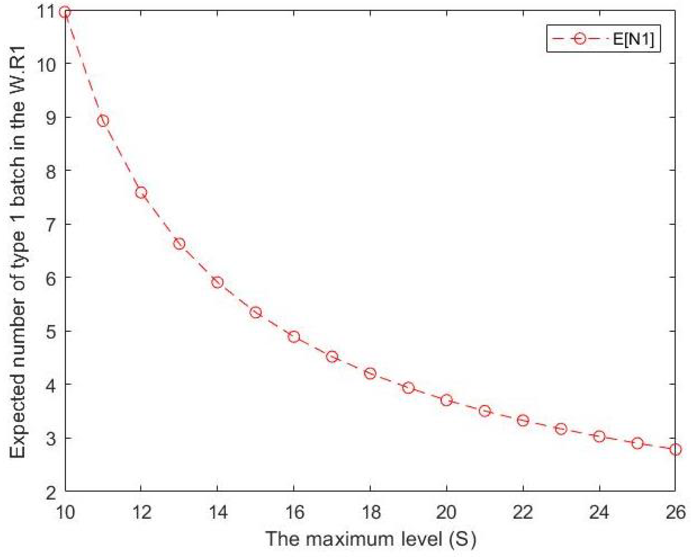
• From Figure 3 and Figure 4, we can see that the expected number of type j batches in the waiting room for type j$\left(E\left[N_j\right]\right)$ decreases as S increases where $j=1,2.$ In other words, from the beginning of the maximum inventory level S onwards, we can conclude that the expected number of type j batches in the waiting room for type j is inversely proportional to the maximum inventory level.
  

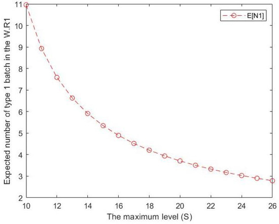  Figure 3. Effect of S on expected number of type 1 customers in the waiting room for type 1.
  

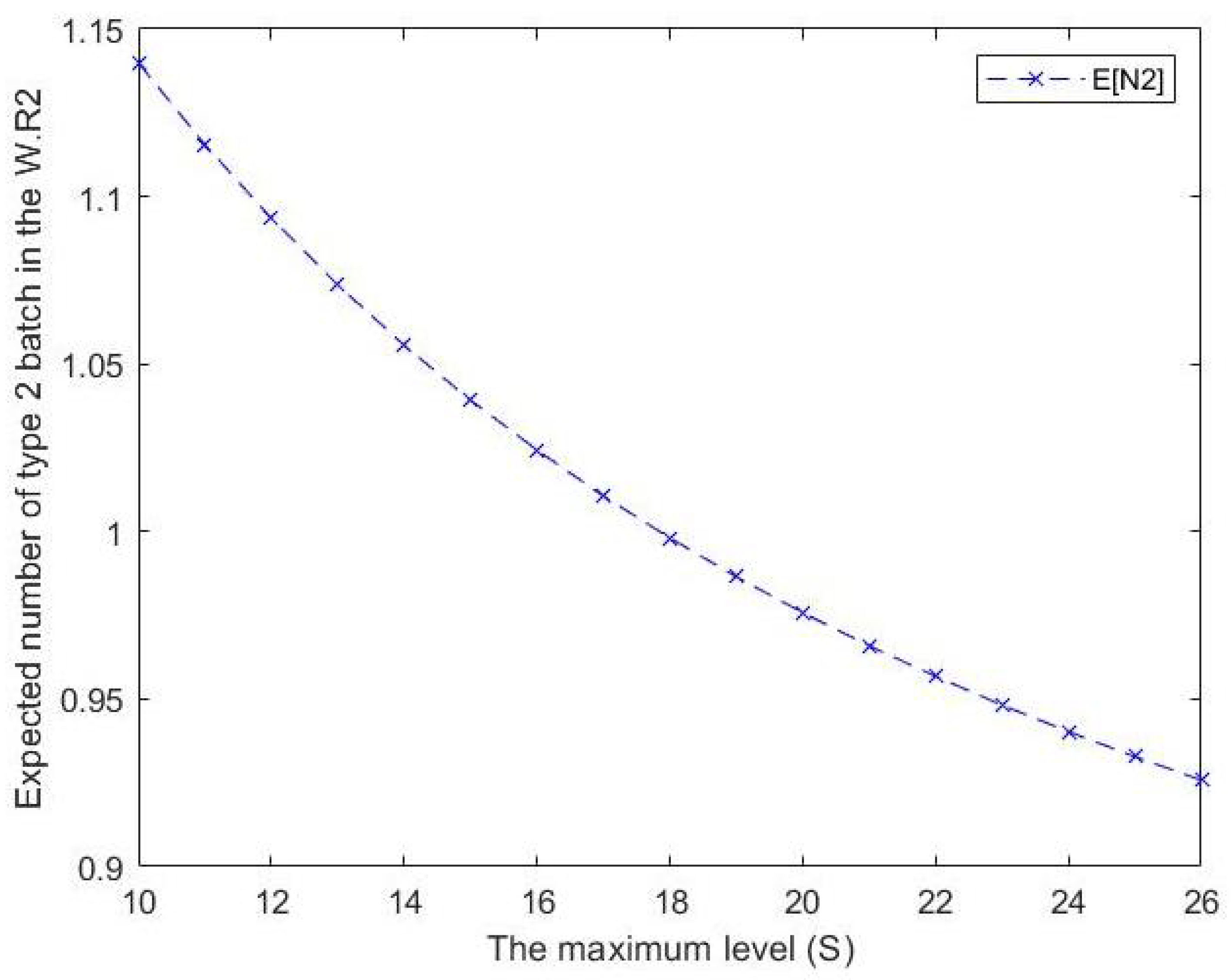
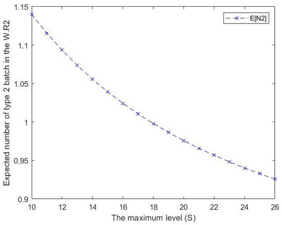  Figure 4. Effect of S on expected number of type 2 customers in the waiting room for type 2.
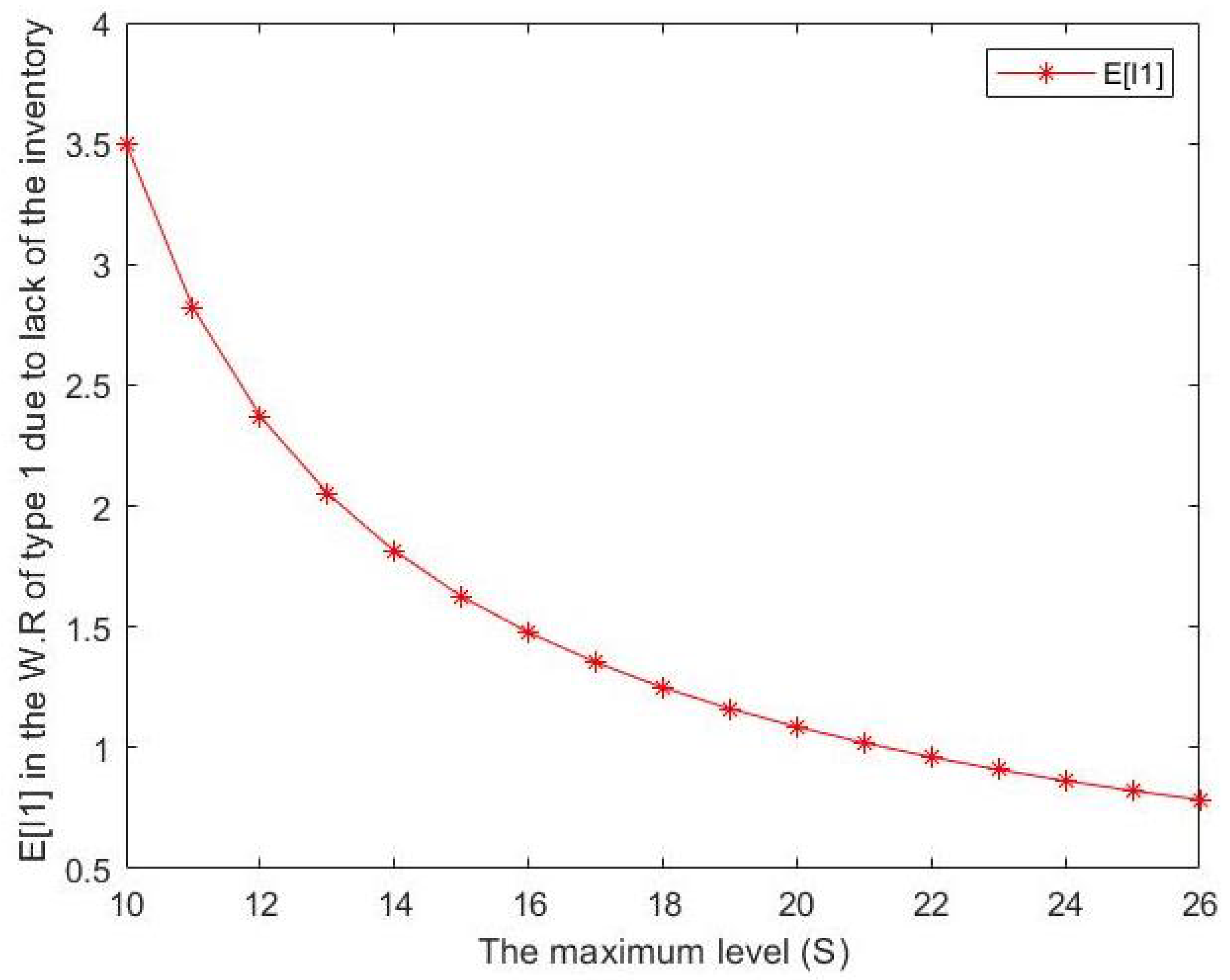
• From Figure 5 and Figure 6, we can notice that the expected number of type j batches in the waiting room for type j due to lack of the inventory $\left(E\left[I_j\right]\right)$ decreases when S increases where $j=1,2.$ Although a slope-like decrease can be seen in $E\left[I_1\right]$, and a gradual, steady decline can be observed in $E\left[I_2\right]$, for both cases, the maximum inventory level S is considered to be inversely proportional to $E\left[I_j\right]$.
  

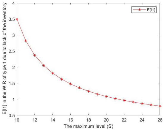  Figure 5. Effect of S on expected number of type 1 customers in the waiting room for type 1 due to lack of inventory.
  

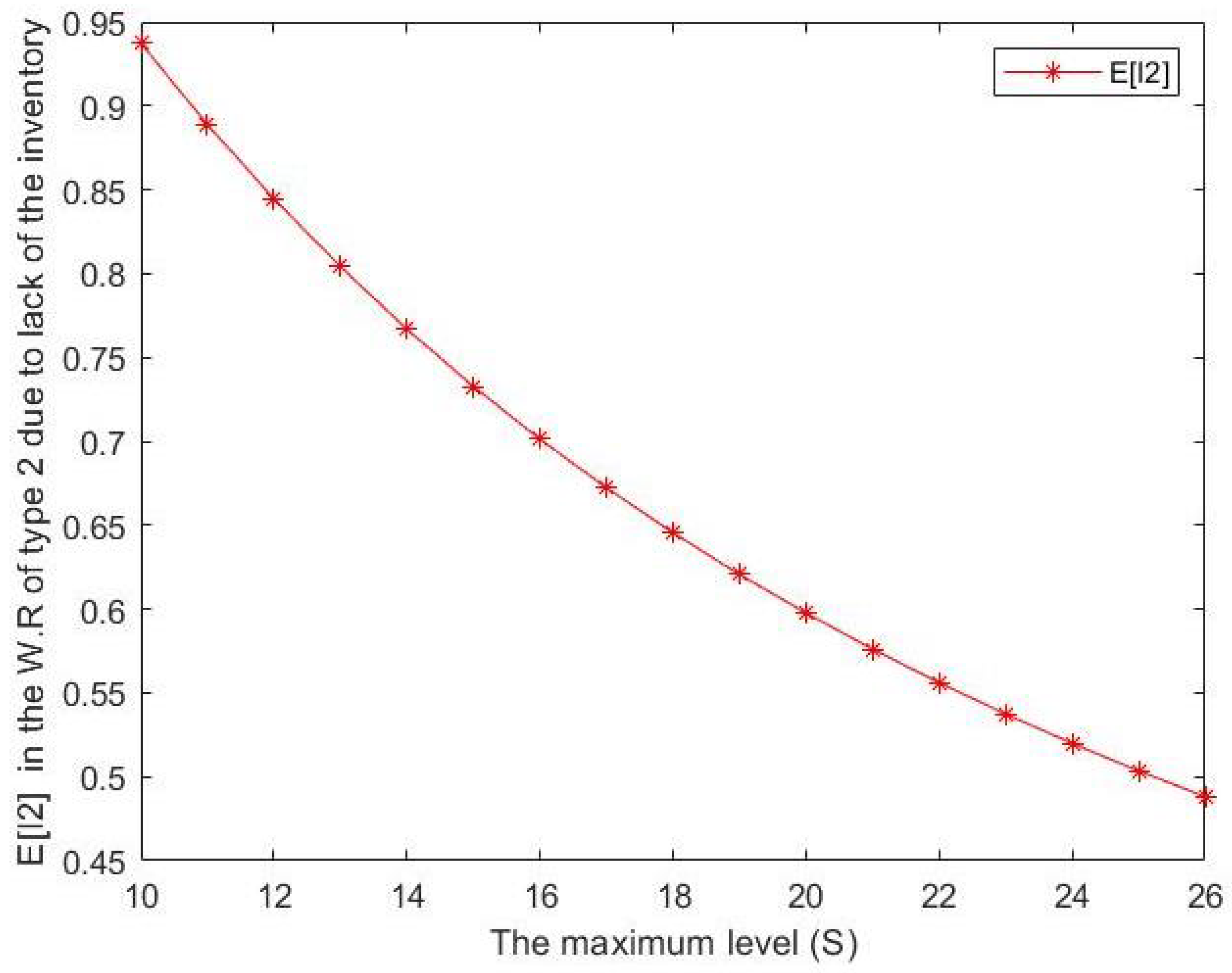
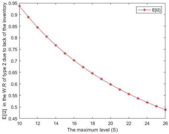  Figure 6. Effect of S on expected number of type 2 customers in the waiting room for type 2 due to lack of inventory.
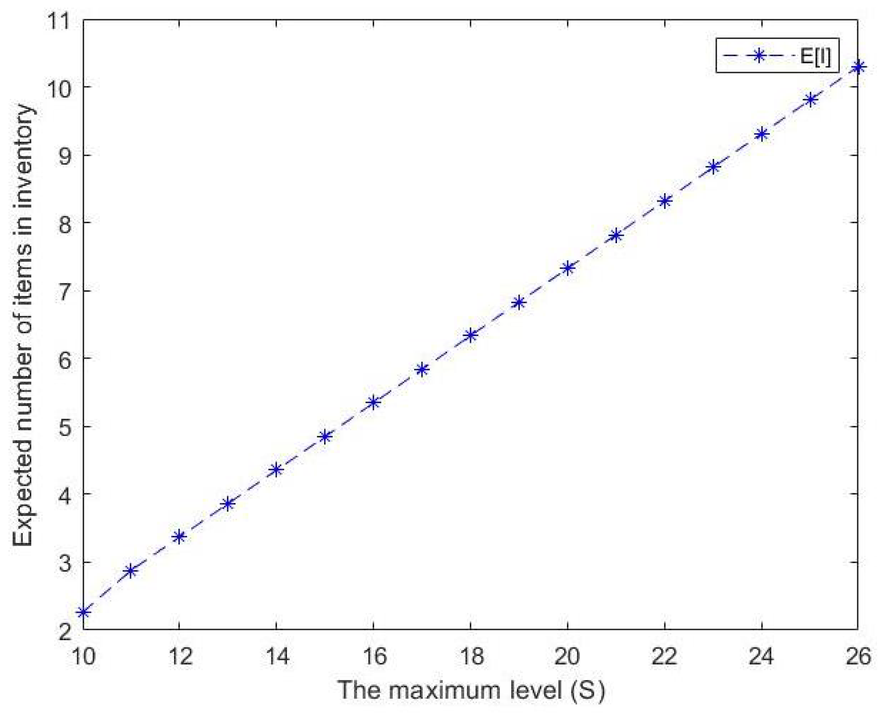
• Additionally, we note from Figure 7 that the expected number of items in inventory $E\left[I\right]$ increases as S increases. In other words, we can note a stable increase in the maximum inventory level and the expected number of items in inventory $E\left[I\right]$. The maximum inventory level is directly proportional to $E\left[I\right]$.
  

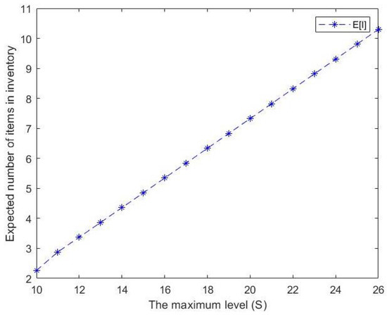  Figure 7. Effect of S on expected number of items in inventory.
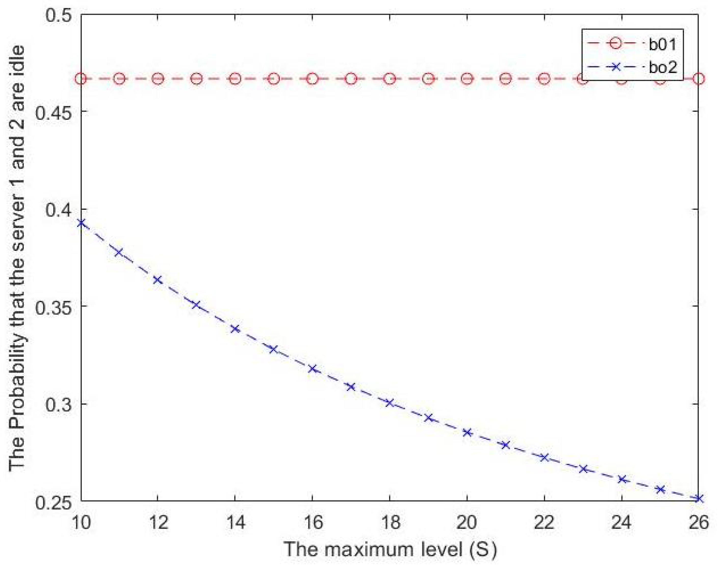
• From Figure 8, we can see that the probability that the server 2 is idle $\left(b_0^2\right)$ decreases as S increases. However, when the maximum inventory level S increases, there is almost no change in the probability that the server 1 is idle $\left(b_0^1\right)$. Simply, a downward trend can be observed in $b_0^2$ while $b_0^1$ experiences a period of stability.
  

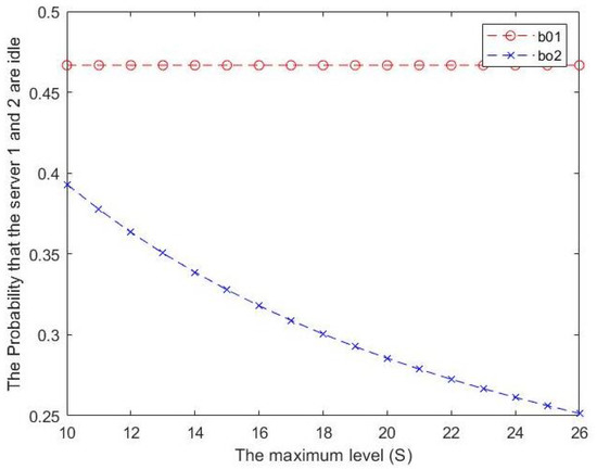  Figure 8. Effect of S on the probability that servers 1 and 2 are idle.

7. Optimization Problem

Based on the above performance measures, we construct a cost function to check the minimality of the expected total cost.

We define the expected total cost $\left(ETC\right)$ per unit of time as:

$$ETC=\sum _{j=1}^k{R}_{j}E\left[N_j\right]+\sum _{j=1}^k{V}_j^{\prime }{b}_0^j+L_{1}E\left[I\right]+\frac{L_2}{E\left[T\right]}$$

(16)

where:

•

$E\left[N_j\right]=$ Expected number of type j customers in waiting room j for $j=1,2,\dots ,k.$

•

$b_0^j=$ Fraction of time server j is idle for $j=1,2,\dots ,k.$

•

$E\left[I\right]=$ Expected number of items in inventory.

•

$E\left[T\right]=$ Expected value of cycle length for reorder point.

•

$R_j=$ holding cost/customer of type j/ unit of time in waiting room j for $j=1,2,\dots ,k.$

•

$L_1=$ holding cost/unit/unit time.

•

$V_j^{\prime }=$ idle time cost of server j for $j=1,2,\dots ,k.$

•

$L_2=$ fixed ordering cost for each reorder point.

We fix $s=3;\lambda =4;p_1=0.4;p_2=0.6;{\mu }_1=3;{\mu }_2=2;\theta =0.6;R_1=\$10;R_2=\$11;L_1=\$12;V_1^{\prime }=\$6;V_2^{\prime }=\$7$ and $L_2=\$25.$ Then, we compute the effect of S on $E\left[T\right]$ and $ETC$ as mentioned in Table 4.

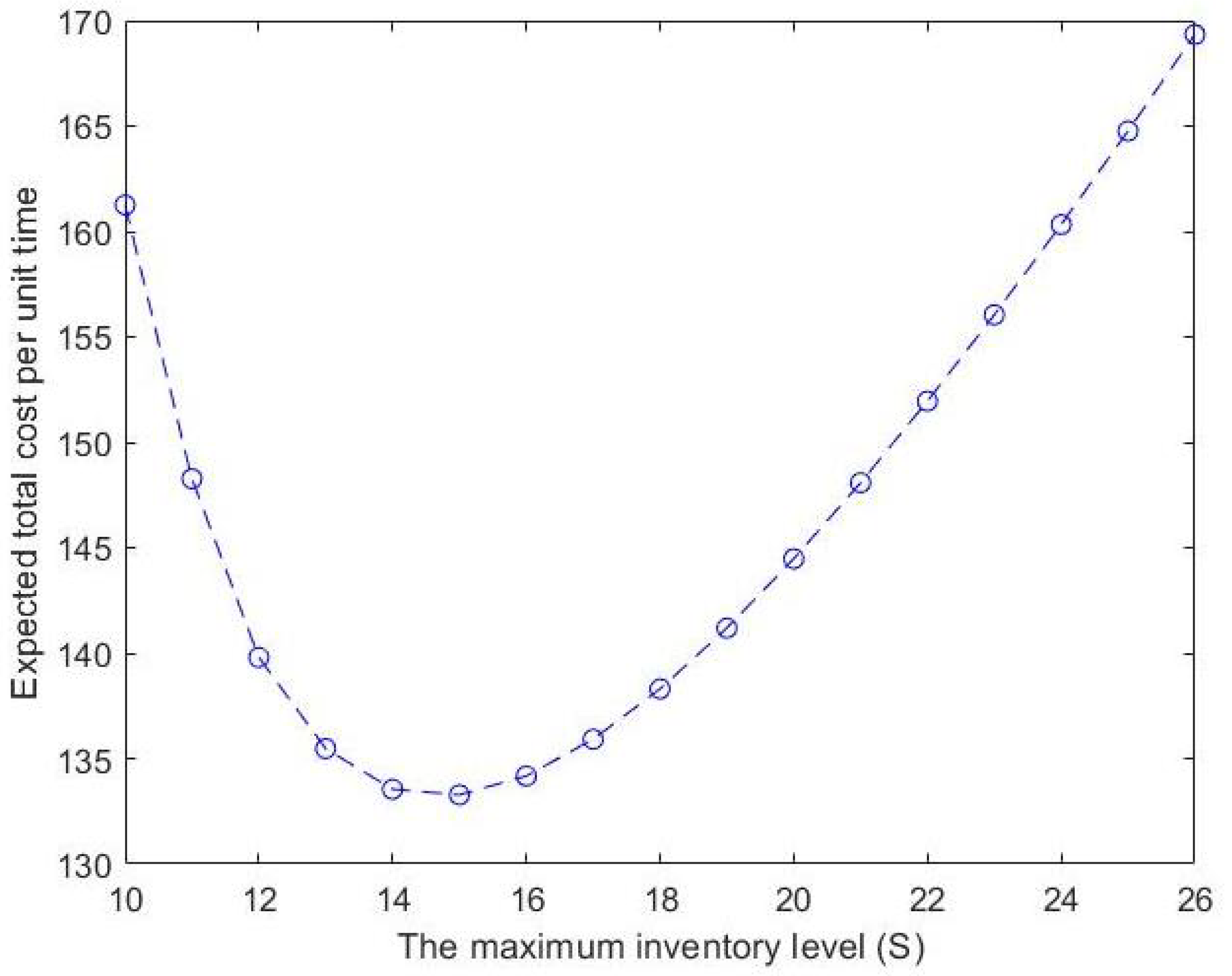
From Table 4 and Figure 9, we can realize that the expected total cost (ETC) per unit of time first decreases with the increase in this maximum inventory level S, reaches a minimum value $ETC=\$133.2777$ when $S=15$ and then starts increasing. In other words, the cost function is convex. Therefore, the optimal value of the expected total cost $\left(ETC\right)$ per unit of time is $ETC=\$133.2777$ when $S=15$ for this example.

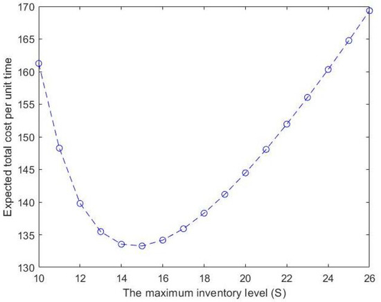
Figure 9. Effect of S on the expected total cost (ETC).

8. Conclusions

In this paper, we studied a queueing inventory system with batch arrival and batch service processes having many servers. Some performance measures were provided. Numerous experiments have been conducted and the inference drawn from them. We studied the effect of the maximum inventory level on performance measures. Additionally, we computed the optimal value of the expected total cost per unit of time. In a future study, we propose to extend the problem discussed in this paper to the batch marked Markovian arrival process and batch Markovian service process (BMMAP and BMMSP, respectively). Furthermore, the processing of items by the servers as described in [12] will be considered. The findings in this paper are proposed to be extended to flexible manufacturing when customers of distinct types demand distinct types of inventory.

References

- Niranjan, S.P.; Indhira, K. A review on classical bulk arrival and batch service queueing models. Int. J. Pure Appl. Math. 2016, 106, 45–51. [Google Scholar]
- Li, W.; Fretwell, R.J.; Kouvatsos, D.D. Performance analysis of queues with batch Poisson arrival and service. In Proceedings of the 13th International Conference on Communication Technology, Jinan, China, 25–28 September 2011; pp. 1033–1036. [Google Scholar]
- Jayaraman, R.; Matis, T.I. Batch Arrivals and Service—Single Station Queues. In Wiley Encyclopedia of Operations Research and Management Science; Wiley: Hoboken, NJ, USA, 2010. [Google Scholar] [CrossRef]
- Baruah, M.; Madan, K.C.; Eldabi, T. A batch arrival single server queue with server providing general service in two fluctuating modes and reneging during vacation and breakdowns. J. Probab. Stat. 2014, 2014, 319318. [Google Scholar] [CrossRef]
- Chen, A.; Pollett, P.; Li, J.; Zhang, H. Markovian bulk-arrival and bulk-service queues with state-dependent control. Queueing Syst. 2010, 64, 267–304. [Google Scholar] [CrossRef]
- Banerjee, A.; Gupta, U.C.; Sikdar, K. Analysis of finite-buffer bulk-arrival bulk-service queue with variable service capacity and batch-size-dependent service. Int. J. Math. Oper. Res. 2013, 5, 358–386. [Google Scholar] [CrossRef]
- Sikdar, K.; Samanta, S.K. Analysis of a finite buffer variable batch service queue with batch Markovian arrival process and server’s vacation. Opsearch 2016, 53, 553–583. [Google Scholar] [CrossRef]
- Al Maqbali, K.A.K.; Joshua, V.C.; Krishnamoorthy, A. On a Queue with Marked Compound Poisson Input and Exponentially Distributed Batch Service. In Distributed Computer and Communication Networks. DCCN 2021; Communications in Computer and Information Science; Vishnevskiy, V.M., Samouylov, K.E., Kozyrev, D.V., Eds.; Springer: Cham, Switzerland, 2022; Volume 1552. [Google Scholar] [CrossRef]
- Adan, I.J.B.F.; Resing, J.A.C. Multi server Batch service Systems. Stat. Neerl. 2000, 54, 202–220. [Google Scholar] [CrossRef]
- Chakravarthy, S.R.; Dudin, A.N. A multi-server retrial queue with BMAP arrivals and group services. Queueing Syst. 2002, 42, 5–31. [Google Scholar] [CrossRef]
- Krishnamoorthy, A.; Joshua, A.N. A BMAP/BMSP/1 queue with Markov dependent arrival and Markov dependent service batches. J. Ind. Manag. Optim. 2020, 17, 2925–2941. [Google Scholar] [CrossRef]
- Krishnamoorthy, A.; Joshua, A.N.; Kozyrev, D. Analysis of a Batch Arrival, Batch Service Queuing-Inventory System with Processing of Inventory While on Vacation. Mathematics 2021, 9, 419. [Google Scholar] [CrossRef]
- Zhao, N.; Lian, Z. A queueing-inventory system with two classes of customers. Int. J. Prod. Econ. 2011, 129, 225–231. [Google Scholar] [CrossRef]
- Yadavalli, V.S.S.; Adetunji, O.; Sivakumar, B.; Arivarignan, G. Two-commodity perishable inventory system with bulk demand for one commodity articles. South Afr. J. Ind. Eng. 2010, 21, 137–155. [Google Scholar]
- ALMaqbali, K.A.K.; Joshua, V.C.; Mathew, A.P.; Krishnamoorthy, A. Queueing Inventory System in Transport Problem. Mathematics 2023, 11, 225. [Google Scholar] [CrossRef]
- Stewart, W.J. Probability, Markov Chains, Queues, and Simulation: The Mathematical Basis of Performance Modeling; Princeton University Press: Princeton, NJ, USA, 2009. [Google Scholar]
Disclaimer/Publisher’s Note: The statements, opinions and data contained in all publications are solely those of the individual author(s) and contributor(s) and not of MDPI and/or the editor(s). MDPI and/or the editor(s) disclaim responsibility for any injury to people or property resulting from any ideas, methods, instructions or products referred to in the content. |
© 2023 by the authors. Licensee MDPI, Basel, Switzerland. This article is an open access article distributed under the terms and conditions of the Creative Commons Attribution (CC BY) license (https://creativecommons.org/licenses/by/4.0/).