1. Introduction
It is well-known that under the risk-neutral measure for pricing, the classic model of Heston [
1] as a set of stochastic differential equations (SDEs) can show the stock option value by considering that the volatility is no longer constant. In fact, it follows the dynamic below with the state vector
:
wherein the variance and the stock processes are
,
, the volatility of volatility is
, the riskless fixed interest rate is
and
. Here
determines the adjustment’s speed of the volatility to the mean
and
are two kinds of Brownian motion. In order to
, the condition of Feller should be satisfied as
.
The model (
1), which is also known as a generalization of the model of Black–Scholes [
2], could be extended further if the interest rate follows a special dynamic as well. There are two well-known models in the literature that take both the interest rate and the volatility to be as stochastic processes: that is, the Heston–Cox–Ingersoll–Ross (HCIR) [
3] and the Heston–Hull–White (HHW) models [
4]. For more information, see [
5,
6].
The model of HHW with the correlation parameters
,
,
could be given in what follows [
4]:
where
represents the process of the rate of interest at time
. In (
2), the positive function
b is given, and
is a new kind of Brownian motion. Here, the parameters
,
are real positive constants.
It is necessary to explain the usefulness of the pricing model using the Heston model combined with the Hull–White model for the market and investors. In fact, as long as the interest rate follows a stochastic dynamic, then pricing would result in more accurate simulation results in equity markets at which the interest rates are no longer constant [
7,
8]. For further related discussions, one may refer to [
8] and the references cited therein.
By employing the dynamics in (
2), the value of a European option could be obtained in the form of the following PDE [
9]:
where
, and
r are the asset price, instantaneous variance, and the rate of interest, respectively. The initial condition, which is known as the payoff function for the call case, could be written as follows:
wherein
K is the price of strike.
The conditions of the boundary along the spatial variables
can be written as [
10]
Note that for the case when
, the PDE (
3) is degenerate, and no boundaries must be imposed [
11].
It is worthwhile to note that to achieve calibration targets in the market, option pricing is an important tool. To price derivative securities, different types of significant models are taken into account and investigated, leading to a set of numerical solvers. The HHW PDE (
3) for the general case does not have a closed-form solution, which turns our attention to efficient numerical methods automatically.
A pioneering numerical method for pricing options is the finite difference (FD) method [
12], which is mainly based on employing uniform discretization nodes, laying a uniform grid on the independent variables of the PDE problem and then transforming the continuous problem into a set of discrete ones.
Another well-performing approach that inherits both from the FD and the radial basis function (RBF) schemes is the local RBF-FD scheme [
13,
14,
15]. For further reading, one may refer to [
16,
17,
18].
Here, the major target is to present a new numerical solver for the simulation of (
3) based on the RBF-FD methodology, which results in block sparse matrices. This is mainly because (
3) is a 3D problem with variable coefficients at which there are three mixed derivatives. Thus, the numerical methods must be designed for this purpose carefully. The RBF-FD formulations are written so as to be applied on graded meshes in which there is a clear concentration on the hot area.
The rest of this article is structured as follows. First, in
Section 2, we review some of the efficient ways of producing graded meshes along the spatial variables to focus more on the hot area of the 3D PDE problem (
3) [
19]. Then, in
Section 3, the RBF-FD weighting coefficients for a new RBF are constructed and proven to converge on graded meshes. The estimations can be considered and simplified on uniform meshes as well.
Section 4 proposes our RBF-FD solver with attention on the financially important area, in which the initial condition of the PDE problem has non-smoothness. The stability of the solver is given in detail in
Section 5 to show how and under what conditions the proposed solver is stable for solving (
3). Then,
Section 6 presents a discussion of the usefulness and applicability of the proposed formulas. Some numerical tests are furnished along with numerical simulations. Ultimately, a conclusion of the work is given in
Section 7.
2. Mesh Generation
The HHW 3D model is defined on
. The merit of the HHW model is that it can take negative rates of interest, unlike the HCIR model at which the interest rate must always be positive [
20].
It is now obvious that to price under the HHW model, we first need to localize the domain as follows:
where
are real positive constants.
It is not that clear what to choose exactly for the
,
, and
in order to get the optimal numerical domain. However, to impose the boundary conditions as well as to reduce the error caused by truncating the domain, it would be better to choose them as far as possible and employ graded meshes at which the focus is on the important area of the problem. Here, the financially important area of the problem (
3) is the region at which the underlying asset price tends to the price of the strike, the spontaneous variance tends to zero, and the interest rate tends to a special small value such as the fixed risk-free interest rate.
To proceed, we assume that
is a partition for
. Now, a well-performing and popular graded mesh could be defined as follows [
21] (
):
wherein
and
are
m uniform points, while we also have
We also take into account that
and
. The parameter
controls the node density around
. Additionally, we define
where
is a proper choice in (
13), while
,
, and
.
Now, the discretized points along
v, i.e.,
are given as
where
provides a density around
. In this paper, we employed
, where
. Additionally for
,
stand for uniform nodes furnished as follows:
Finally, the graded points alongside
r are given by
where
and
is a positive number. It is considered
,
. Note that the variables
are local counter variables throughout the paper.
3. Constructing the RBF-FD Weights
Now, the famous inverse quadratic (IQ) RBF is considered as follows ([
22], [Chapter 4]) (
):
where
s is the parameter of shape and
stands for the Euclidean distance.
Remark 1. The motivation behind choosing this RBF is based on the recent work [23] that states that the IQ-based RBF-FD weights could be constructed theoretically more easily than multiquadrics (MQs) RBFs, which are available in the literature [24]. Besides this, another motivation stems from the fact that the IQ is an infinitely smooth RBF; under mild conditions [25], its one-dimensional function interpolants that are analytic inside a strip exponentially converge. To find weights of the RBF-FD methodology on a graded mesh having three points, by considering
L as a linear operator of approximation in the RBF-FD methodology, one can start with [
26]
This leads to
unknowns for
equations while the solutions are
. Note that
L is not a differential operator and is sometimes used for the discretization of the PDE problem. To illustrate further, in this section, by (
19), we only focus on approximating the (1D) function derivatives. So, a derivative of the function is approximated by a combination of (three) adjacent nodes while the weights are unknown.
Hence, for
, we obtain
and write (
19) as
wherein
and
f are the approximate and exact values, respectively.
Remark 2. Recalling that the error equation at the point can be defined by The reason for mentioning the error is to say how accurate the RBF-FD estimations arising from (19) are when we approximate different function derivatives by considering only three adjacent non-uniform points. Theorem 1. When estimating the first derivative of the function f, the equation of error by the IQ RBF-FD procedure (21) is obtained as follows:where Proof. The proof is similar to [
24], and hence it is omitted. □
To compute the weights of the function’s second derivative, we write for
:
Hence, we can state the following theorem.
Theorem 2. When estimating the second derivative of the function f, the equation of error by the IQ RBF-FD procedure (26) is obtained viawhere and Proof. The proof is similar to [
24], and hence it is omitted. □
An effective procedure could be here used for the selection of the shape parameter in numerical implementations, as comes next:
where
are the increments along the variable mesh. The motivation behind choosing the shape parameter as (
31) is that we must select
c to be larger than
h, i.e.,
, and also an adaptive
c that changes based on the number of discretization points will affect positively more on the numerical results than a constant shape parameter. On the other hand, after using a trial and error approach, we found that a larger value as the coefficient, i.e., 5, in (
31), will tend the RBF-FD methodology towards the FD approach, and a smaller value will cause some instability issues. Thus, coefficient 5 can help us to get efficient numerical results.
Now, an introduction on how RBF-FD works is necessary to discuss the different stages of the methodology. Some remarks are in order:
In fact, the weights we obtained by now are used in an initial step by considering three points of the stencil. Each time, three interior points of the stencil are considered (in a loop), and the weights are computed.
These values along with the weights corresponding to the first and last nodes are grouped together in a matrix, which we call the differentiation matrix in the next section.
Note that after computing the matrices, the final matrix will not be changed during the time stepping process, as we discuss in the next section as well.
The computed weights change only when the three adjacent nodes of the stencil or their spacings (h or w) change.
4. Numerical Method
To construct our RBF-FD solver, first, the method of lines (MOL) is employed [
27,
28], in which all the spatial variables are discretized to attain a system of linear ordinary differential equations (ODEs). Hence, let us define two differentiation matrices having the weights for the RBF-FD procedures on graded meshes described of
Section 2 as follows:
and
We here discuss the procedure along
s, while the procedure along other variables would be similar. For the discretization nodes located on the boundaries, we point these out as follows. The formulations (23)–(25) and (28)–(29) would be fruitful for rows two to the row before the last one. Accordingly, for the nodes located on the sides, we may use sided FD approximations as follows:
and
wherein
.
Similarly, for the four nodes
,
,
,
, we can obtain (see e.g., [
29])
where
, and
h stands for the maximum space width along the considered nodes of the stencil.
Recall that using a similar spirit of logic for the point
, we could calculate the second-order approximate formulation and its corresponding weights as follows:
Note here that for the sake of simplicity and since the function does not have any fluctuations in practical consideration, we may expand it up to zeroth order in order to estimate it by a scalar, i.e., . The motivation behind this is to get rid of of a time-variable coefficient function and thus a time-varying matrix. To illustrate further, by this consideration, we simplify the numerical solver as much as possible.
Now, let ⊗ denote the Kronecker product, and the
identity matrix
is given where
,
is the
identity matrix for
s, and for
and
similarly. Thus, now we can encapsulate the whole numerical procedure for the 3D case as follows:
The square matrices
,
,
,
,
, and
are derived via the corresponding weights similarly. In addition, the diagonally sparse matrices
,
and
can be expressed as
Taking all the weights into matrices, it would be possible to transfigure the PDE into a system of ODEs to price (
3) as follows:
wherein the vector of unknowns is
After considering the boundary conditions (
5), a system of ODEs can be attained as follows:
where
is the system matrix consisting of the boundary conditions. This means that the boundary conditions given in (
5) must be imposed to appropriate rows of
A. This can be done by writing (
5) in time differentiation form, and thus we obtain a new matrix
.
6. Simulation Results
The target of this section is to compare the efficacy of various solvers in order to solve (
3) on the same numerical domain when
,
,
year and
. The methods are summarized as follows:
The solver proposed in [
21] on graded meshes is shown by HM, which stands for Haentjens’s method. The motivation behind choosing HM is that it is one of the most fundamental and efficient methods for solving (
3),
The second-order FD method with uniform node distribution along space and the explicit first-order Euler’s method shown by FD, see e.g., [
10],
In fact, RBF-FD is a general name for the procedure, but when the specific IQ RBF is used along with the time-stepping solver (
44), then we call it RBF-FDM. The reason for choosing the explicit first-order Euler’s method for the HM and FD is because this time-stepping method has been used for these solvers in [
21]. All the compared solvers are written in Mathematica 12.0 [
32].
Here, the CPU time is reported in seconds. Besides this, the absolute error is computed by
wherein
and
are the referenced and numerical solutions, respectively.
is selected from the already published literature [
10].
Noting that the function
b is normally defined as follows:
where
,
,
are constants, and
. Note that
and
are not zero. The following tests are discussed in this section.
Example 1 ([
10])
. In this test, the following sets of parameters are considered: , , , , , , , , , , , where the reference value is . Example 2 ([
10])
. A different set of parameters is considered in this test to compare the results of different solvers: , , , , , , , , , , , where the reference value is . Since the numerical domain along the variable
s is longer than the other two variables, it is convenient to consider a greater number of discretization points even based on graded meshes along the underlying asset price. Clearly, the choice of the temporal step size mostly depends on the choice of the time integrator and its stability region. For HM and FD, the radius is of course lower than the time integrator for the proposed solver, which is a fourth-order method with the stability condition (
54).
The numerical pieces of evidence are put together in
Table 1 and
Table 2. Both indicate that by increasing the number of discretization points, the accuracy is improved for all solvers, but the graded meshes for the proposed solver along its efficient structure help us to obtain higher accuracies as quickly as possible. The time to compute the weights of the RBF-FD methodology are included here. Actually, the times reported here stand for the whole computational time from the very beginning of considering the input values until the final interpolations and printing the result.
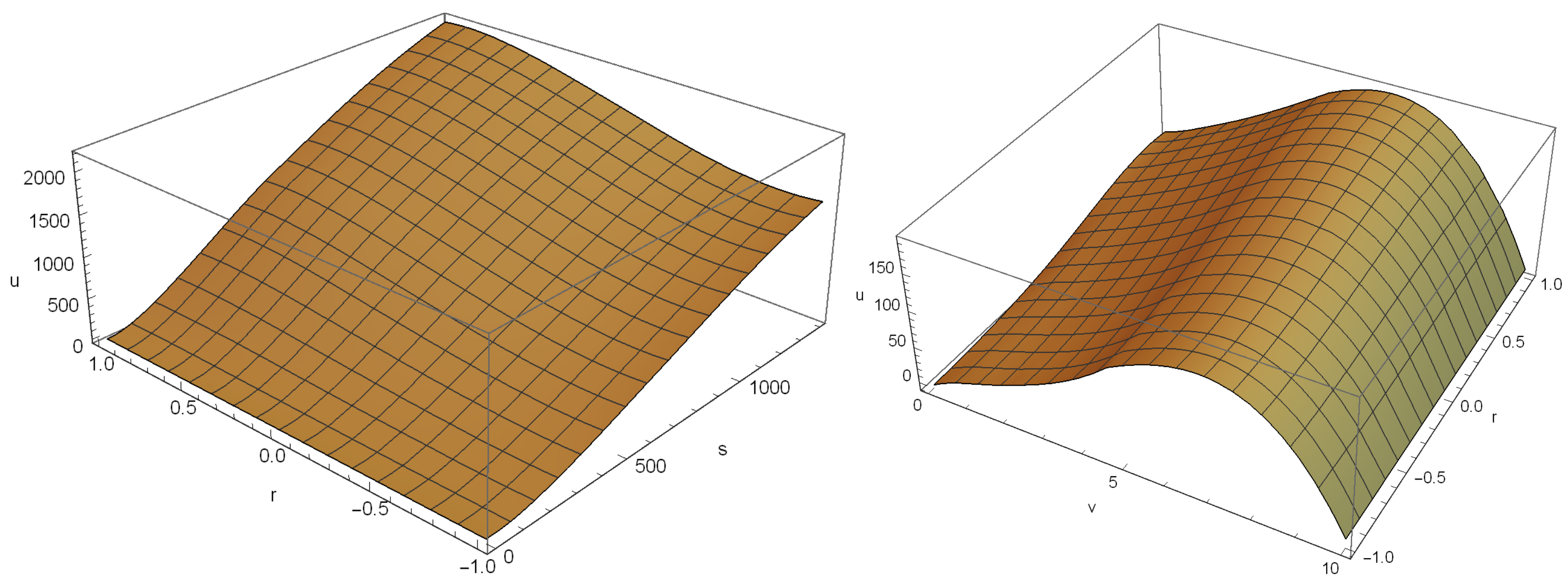
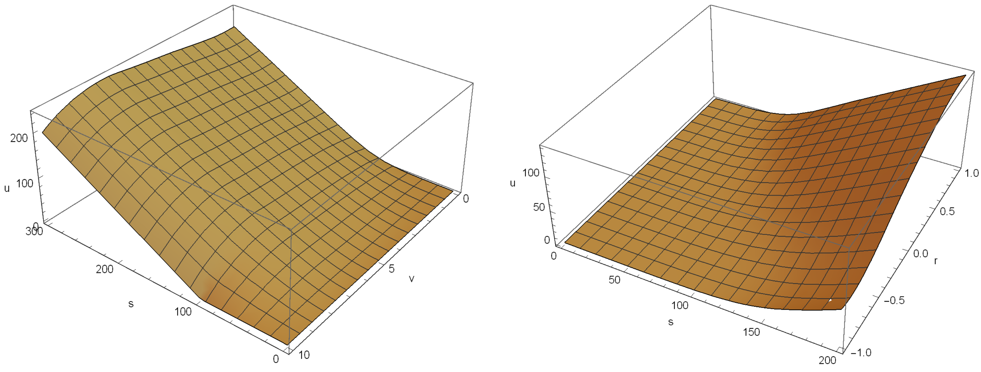
For the case of
,
, and
in Example 1, the numerical solution has been plotted in
Figure 1 as well. It shows that the numerical solution for the considered cut is positive without oscillations. Similarly, in
Figure 2 for the Example 2, two cuts of the numerical solution are provided to re-support this.
An inquiry may arise regarding why we did not choose the same number of spatial steps and time-steps for the different methods in
Table 1 and
Table 2. The answers lie in the fact that we use a greater number of nodes along
s and then
v, since their computational domains are bigger, i.e., the bigger the domain, the greater the number of nodes used. In addition, of course, smaller temporal step-sizes are used for the FD and the HM, since their time-stepping solver has a smaller stability region. The methods can simply be compared by considering their elapsed CPU times (roughly) and checking the absolute errors.
The Greek characters are significant to calculate in order to show the stability of a numerical method in option pricing. Hence,
Figure 3 shows the delta and gamma and confirms a stable numerical solution for the proposed approach.
It is commented that the two methods (FD and HM) have some more stability issues in contrast to the RBF-FDM. This is because of the use of a time-stepping method with a larger stability region. The methods FD and HM use the explicit first-order Euler’s method, which of course has a smaller stability region in contrast to (
44).
In
Table 1 and
Table 2, it is noticeable that the proposed approach has a slower calculation time as well as higher accuracies. The improved accuracy in terms of absolute errors is mainly due to the application of the RBF-FDM scheme with an appropriate shape parameter, and the lower computational time is mainly due to employing lower temporal step sizes because of using (
44) with larger stability regions.
With the numerical results given in this section, we believe that our fast and stable solver opens a new possibility for efficient and accurate derivative pricing.
We end this section by repeating Example 1 and only by changing
in order to check the numerical results when the Feller’s condition is unsatisfied. Considering RBF-FDM with
,
, and
, the numerical results are given in
Figure 4, confirming the applicability and usefulness of the proposed approach even when the Feller condition is unsatisfied.
7. Summary
Trading based on options can occur in daily market routines. Hence, pricing them when both the interest rate and the volatility follow some stochastic dynamics is of practical interest for risk managers and traders. This work focuses on the significant financial model of HHW as a 3D time-dependent PDE problem and proposes a new solver to expand the relevant literature’s conclusions. In fact, our methodology is to consider graded meshes on all the involved spatial variables in order to concentrate on the financially hot area more. Then, the weighting coefficients for an RBF were constructed on such meshes and proved to have second and first orders to approximate the first and second derivatives of a function. MOL is then applied through extensive compact matrix notations to build up the new solver as a system of ODEs. An explicit but fast time-stepping method was used and the stability of the solver discussed in detail. Computational simulations have validated the applicability of the presented RBF-FD sparse solver for solving the HHW equation.
Investigating how to compute an optimal value for the shape parameter as well as to employ the new efficient method furnished in this paper for other kinds of derivative securities could be conducted in future works in this field of research. Besides, it is recalled that the generalized Stein–Stein model [
7], which is also known as the model of Schöbel–Zhu [
33], can be expressed as a system of two SDEs in a similar way to (
1) but differs in some perspectives. Applying such a consideration along with stochastic interest rates can yield another generalized hybrid model, known as the hybrid Schöbel–Zhu–Hull–White PDE, which is discussed deeply in [
34]. Pricing such a PDE [
35,
36] can be investigated by the localized meshless methods in forthcoming works.


