A Spanning Union of Cycles in Thin Cylinder, Torus and Klein Bottle Grid Graphs ^†

Abstract

In this paper, we propose an algorithm for obtaining the common transfer digraph ${\mathcal{D}}_m^{*}$ for enumeration of 2-factors in graphs from the title, all of which have $m·n$ vertices ($m,n\in N,m\ge 2$). The numerical data gathered for $m\le 18$ reveal some matches for the numbers of 2-factors for different types of torus or Klein bottle. In the latter case, we conjecture that these numbers are invariant under twisting.

1. Introduction

A spanning subgraph of a graph G in which every vertex has two degrees is called a 2-factor of G. It represents the union of cycles which has the same vertex set as G. Specifically, if the number of these cycles is one, then we call it a Hamiltonian cycle. Enumerating and generating Hamiltonian paths are of interest in chemistry, theoretical physics and biophysics related to polymer melting, protein folding [1] and the study of magnetic systems with $O\left(n\right)$ symmetry [2]. It might also be useful in the theory of algorithms [3,4]. Additionally, the path planning problem for robots and machine tools [5] as well as security and intellectual property protection using microelectrode dot array (MEDA) biochips [6] make the study of this problem important in engineering and bioinformatics, especially when G is a grid graph. For a brief overview of the chronology of the research on enumeration of Hamiltonian cycles in different graph families, we refer the reader to [7].

The grid graphs with $m·n$ ($m,n\in N$) vertices on different surfaces can be considered sequences with an index n (or m). The sequences of the numbers of Hamiltonian cycles ($h_m\left(n\right)$) in the rectangular grid graph and the thin and thick cylinders obtained in recent papers revealed some interesting properties. For example, asymptotically equal behavior (when $n\to \infty$) of these sequences in the contractible and non-contractible cases was spotted for the thin cylinder [8]. For the thick grid cylinder, the supremacy of contractible Hamiltonian cycles over non-contractible ones depends on the parity of m [9]. Additionally, the computational data for $m\le 10$ indicated that the coefficient for the dominant eigenvalue in the non-contractible case was equal to one and that the positive dominant characteristic root in the contractible case was equal to the same one associated with the rectangular grid graph [10].

With the aim to find some conclusions which can help in proving the above-mentioned properties, we started the investigation of 2-factors in these graphs as a generalization of Hamiltonian cycles. The research in [11,12] was dedicated to the rectangular $R{G}_m\left(n\right)$, thick cylinder $Tk{C}_m\left(n\right)$ and Moebius strip $M{S}_m\left(n\right)$ grid graphs. We proposed an algorithm for obtaining 2-factor transfer digraphs common for all three classes and explored its structure. In this paper, we continue with three new classes of grid graphs: the thin cylinder $Tn{C}_m\left(n\right)$, torus $T{G}_m^{\left(p\right)}\left(n\right)$ and Klein bottle $K{B}_m^{\left(p\right)}\left(n\right)$, all of which have $m·n$ vertices.

2. Definitions, Notations and Tools

The structure of (square) grid graphs under consideration allows the grouping of vertices in “columns” and consideration of their edges as “vertical” and “horizontal”.

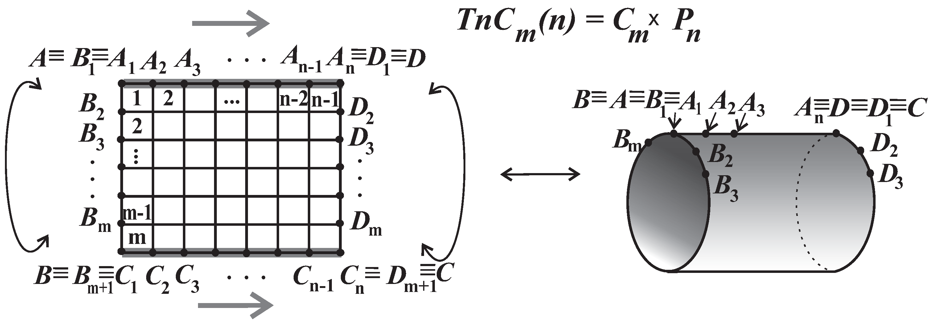
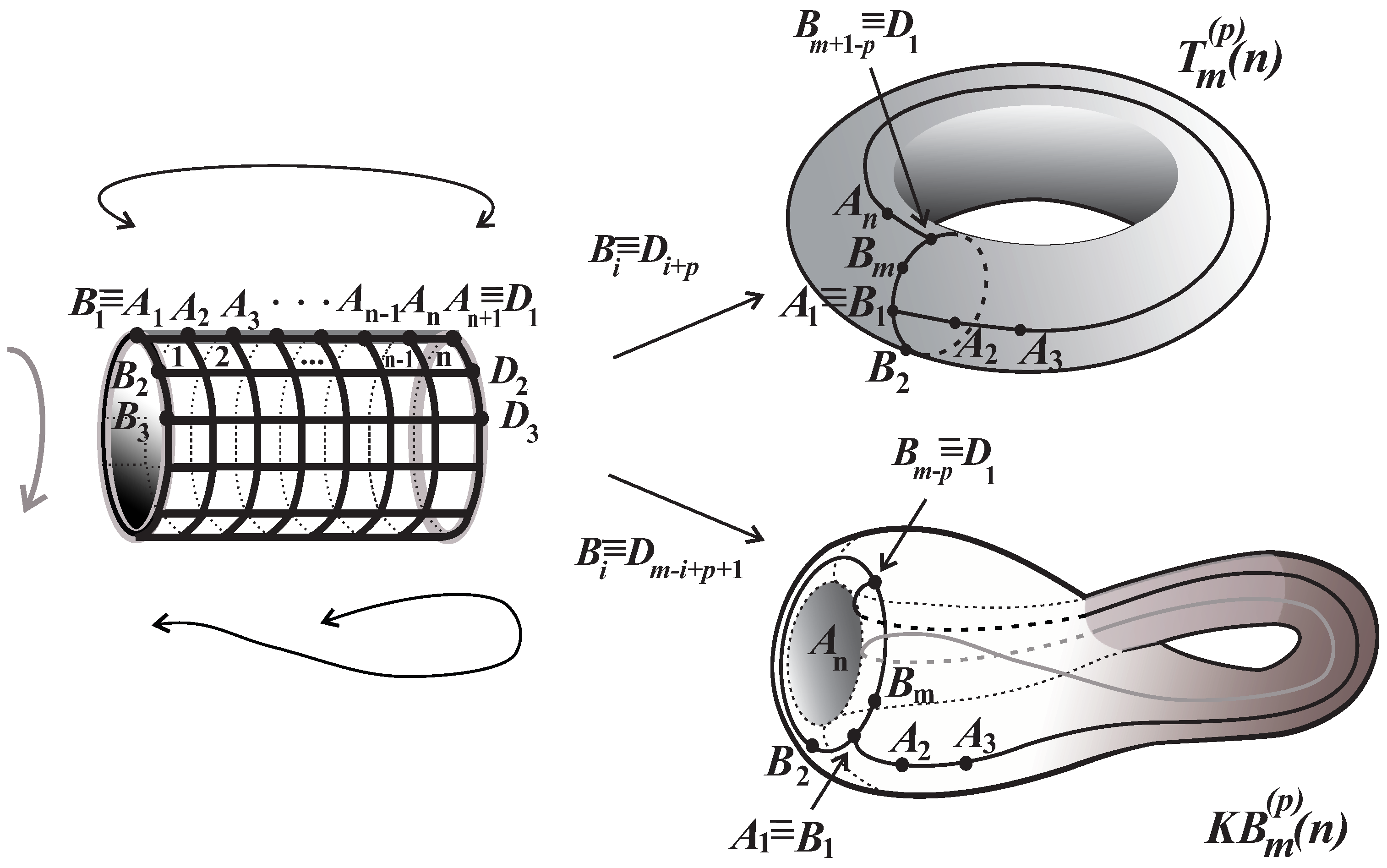
The $Tn{C}_m\left(n\right)\stackrel{\mathrm{def}}{=}{C}_m\times P_n$, where $P_n$ and $C_n$ denote the path and cycle with n vertices, respectively, can be obtained from the rectangular grid graph $R{G}_{m+1}\left(n\right)$$=P_{m+1}\times P_n$ by identification of the corresponding vertices from the first and last rows (in Figure 1, the vertex $A_i$ coincides with $C_i$, both from the ith column, where $i=1,\dots ,n$) without producing (horizontal) multiplying edges. The other two graphs from the title can be obtained from the thin grid cylinder $Tn{C}_m(n+1)=C_m\times P_{n+1}$ by gluing the corresponding vertices from the first and last columns without producing vertical multiplying edges. The identification of corresponding vertices from the first and last columns in $Tn{C}_m(n+1)$ can be achieved in several ways, resulting in the following grid graphs on a torus or Klein bottle surface (see Figure 2).

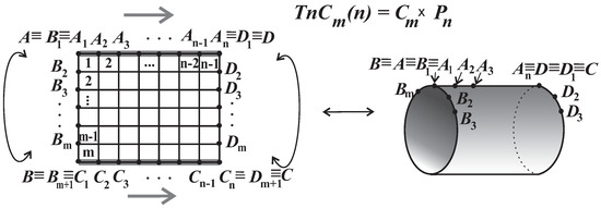
Figure 1. Construction of the thin grid cylinder $Tn{C}_m\left(n\right)=C_m\times P_n$.

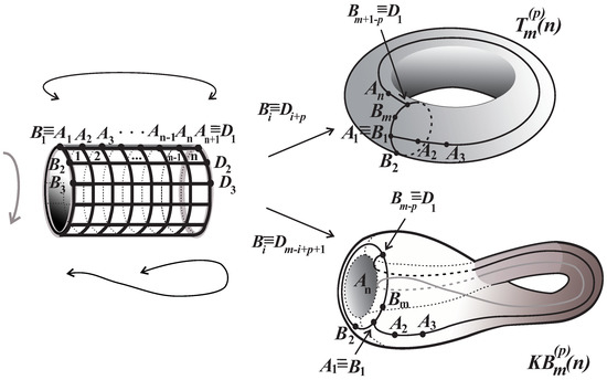
Figure 2. Construction of the torus grid $T{G}_m^{\left(p\right)}\left(n\right)=C_m\times C_n$ and Klein bottle $K{B}_m^{\left(p\right)}\left(n\right)$.

Definition 1.

Let $B_i$ and $D_i$ denote the vertices belonging to the ith row ($1\le i\le m$) from the first and last columns, respectively, in the graph $Tn{C}_m(n+1)$.

The torus (grid) $T{G}_m^{\left(p\right)}\left(n\right)$ ($0\le p\le m-1$) is the graph obtained from $Tn{C}_m(n+1)$ with identification vertices $B_i$ and $D_{i+p}$ for $i=1,\dots ,m$ and without duplicating edges.

The Klein bottle $K{B}_m^{\left(p\right)}\left(n\right)$ is the graph obtained from $Tn{C}_m(n+1)$ with identification vertices $B_i$ and $D_{m-i+p+1}$ for $i=1,\dots ,m$ and without duplicating edges. In both cases, the sign + in subscript is the addition modulo m. The value $m\in N$ is called the width of the grid graph.

Informally, in both cases, we elongated the cylinder and then bent it so that the two ends of the cylinder (i.e., the cycles with vertices $B_1,B_2,\dots ,B_m$ and $D_1,D_2,\dots ,D_m$) came close to each other. Prior to identification, one end of the cylinder was twisted until the corresponding vertices matched. Note that $T{G}_m^{\left(0\right)}\left(n\right)=C_m\times C_n$ is just a special case of the torus grid graph.

For an arbitrary 2-factor of a considered graph of the width $m\in N$, we coded its vertices. To each column, we joined a word over some alphabet of a length m (abbreviated as m-word). These words represent the vertices of the so-called transfer digraph ${\mathcal{D}}_m$. The arcs in ${\mathcal{D}}_m$ reflect the possibility that two m-words appear as adjacent columns. The process of enumeration of 2-factors was reduced to enumeration of some oriented walks in this digraph. Contrary to the case of rectangular, thick cylinder and Moebious strip grid graphs, where the words assigned to the columns of vertices are linear, for the graphs from the title ($Tn{C}_m\left(n\right)$, $T{G}_m^{\left(p\right)}\left(n\right)$ and $K{B}_m^{\left(p\right)}\left(n\right)$ ($0\le p\le m-1;m,n\in N$)), we treated those words as circular ones.

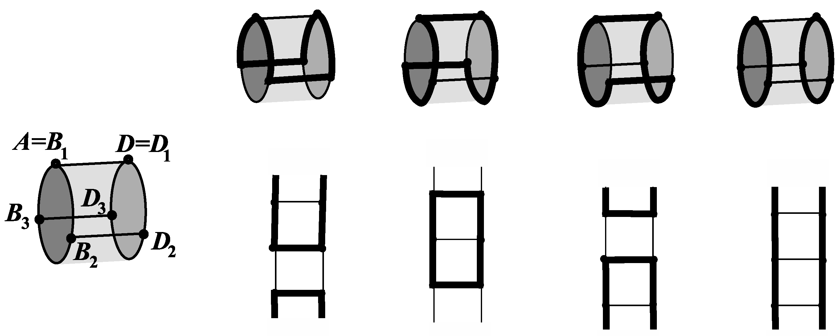
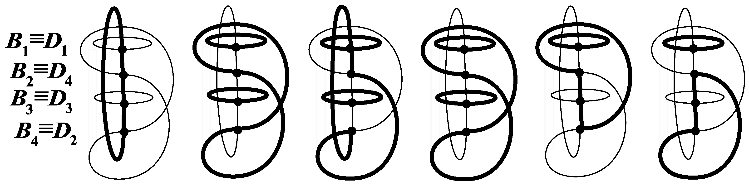
In Figure 3, the grid graph $Tn{C}_3\left(2\right)=C_3\times P_2$ and all its possible 2-factors are shown. With the exception of the last case, all other 2-factors were connected (i.e., Hamiltonian cycles).

Figure 3. The graph $Tn{C}_3\left(2\right)=C_3\times P_2$ with all the possible 2-factors (bold edges) and their flat representations (below).

To be able to “walk to the left, right, upper or down” trough the cycles in a 2-factor of one of our grid graphs, imagine that we “cut and develop in the plane” the surfaces of the considered graph. At first, in the case of the torus $T{G}_m^{\left(p\right)}\left(n\right)$ or Klein bottle $K{B}_m^{\left(p\right)}\left(n\right)$, we “cut” the edges connecting the vertices of the last and first columns. Then, in all three cases, we did the same with the edges connecting the vertices of the last and first rows of the cylinder and developed them in the plane (see Figure 3 below).

Definition 2.

The picture obtained after the described “cutting and developing in the plane", in which the lines corresponding to the edges of the considered 2-factor are bolded, is called the flat representation (FR). In the case of the thin cylinder, by using translation of an infinite number of copies of FR and linking them to each other in a sequence, we obtained the infinite strip grid graph of a width n. In the other two cases, at first we produced the similar infinite strip. Then, we made the copies of it, and using translation (in the case of torus) and glade symmetry (in the case of the Klein bottle), we tiled the whole plane, taking into account that $B_i\equiv D_{i+p}$, $i=1,\dots ,m$ for $T{G}_m^{\left(p\right)}\left(n\right)$, or $B_i\equiv D_{m+p+1-i}$, $i=1,\dots ,m$ for $K{B}_m^{\left(p\right)}\left(n\right)$. The picture of the infinite grid graph obtained from copies of FR is called the rolling imprints (RI).

Figure 4 illustrates this tiling technique for $Tn{C}_m\left(n\right)$ and Figure 5 for $T{G}_m^{\left(0\right)}\left(n\right)$, $T{G}_m^{\left(2\right)}\left(n\right)$, $K{B}_m^{\left(0\right)}\left(n\right)$ and $K{B}_m^{\left(4\right)}\left(n\right)$.

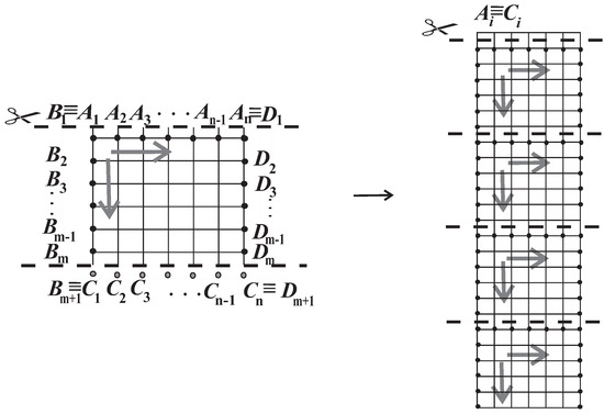
Figure 4. The technique for obtaining rolling imprints using flat representation for $Tn{C}_m\left(n\right)$.

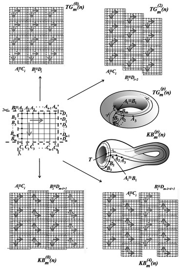
Figure 5. The technique for obtaining rolling imprints using flat representation for $T{G}_m^{\left(p\right)}\left(n\right)$ and $K{B}_m^{\left(p\right)}\left(n\right)$.

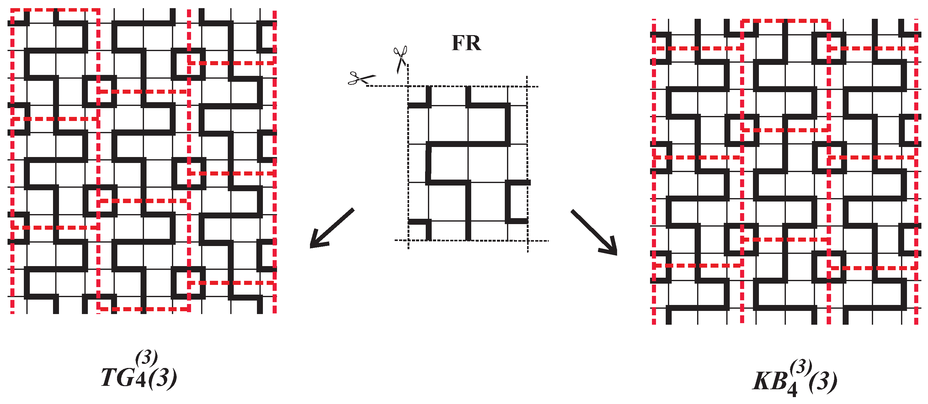
Note that one FR can serve different types or classes of grid graphs (see Figure 6). The concept of rolling imprints was introduced in [10]. Observe that the bold lines in RI determined the 2-factor of the infinity grid graph for all three classes.

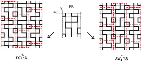
Figure 6. RI of a 2-factor for $T{G}_4^{\left(3\right)}\left(3\right)$ (left) and RI of a 2-factor for $K{B}_4^{\left(3\right)}\left(3\right)$ (right) with their common flat representation (in the middle).

In this problem, we use matrix labeling. Thus, each vertex of the considered grid graph G with $m·n$ vertices is represented with an ordered pair $(i,j)\in \{1,2,\dots ,m\}\times \{1,2,\dots ,n\}$, where i is the ordinal number of the row viewed from top to bottom in FR while j is the ordinal number of the column in FR viewed from left to right:

Definition 3.

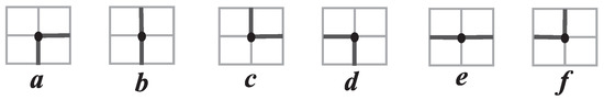
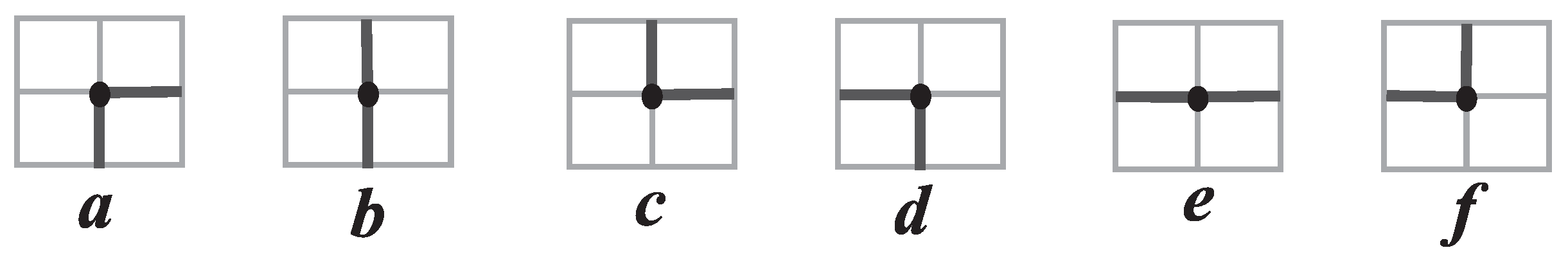
We associate each 2-factor of the observed graph G with the so-called code matrix ${\left[{\alpha }_{i,j}\right]}_{m\times n}$, where ${\alpha }_{i,j}$ is one of six possible labels shown in Figure 7 (called alpha letters) that corresponds to the vertex $(i,j)$ ($1\le i\le m$, $1\le j\le n$). By reading the columns of these code matrices from top to bottom, we obtain the so-called alpha words.

Figure 7. Six possible situations in any vertex for a given 2-factor.

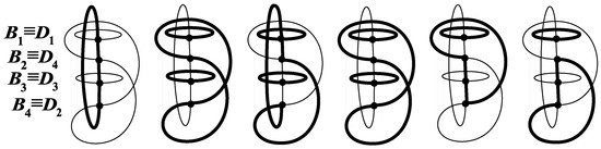
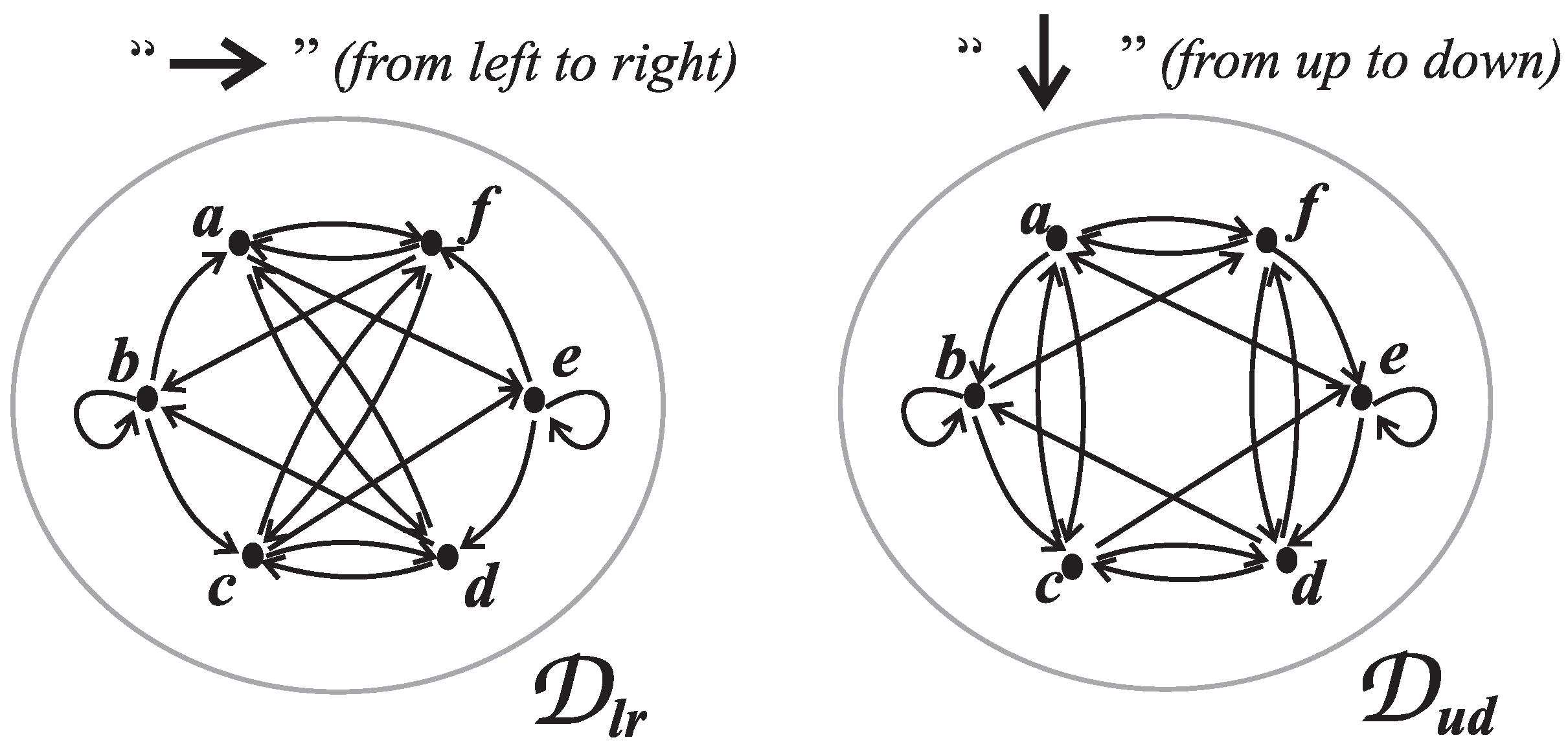
For instance, three alpha words—$facd$, $cedb$ and $dfac$ (following column order)—determined the 2-factors shown in Figure 6. The digraphs ${\mathcal{D}}_{lr}$ and ${\mathcal{D}}_{ud}$, shown in Figure 8, describe the possibility that two alpha letters correspond to two adjacent vertices of G in a 2-factor. Contrary to the case when G is a linear grid graph [11,12], now, these words are circular.

Figure 8. Digraphs ${\mathcal{D}}_{ud}$ and ${\mathcal{D}}_{lr}$.

The organization of the rest of this paper is as follows. In Section 3, by using code matrices, we give a characterization of the 2-factors for each of the grid graphs from the title. Using this characterization and the transfer matrix method [13], we propose algorithms for obtaining the numbers of 2-factors, labeled by $f_m^{TnC}\left(n\right)$, $f_{m,p}^{TG}\left(n\right)$ and $f_{m,p}^{KB}\left(n\right)$, where the integer p refers to the type of grid graph. Additionally, we give some properties of the transfer digraph ${\mathcal{D}}_m$, whose adjacency matrix ${\mathcal{T}}_m$ is the transfer matrix used in these algorithms. In this way, the problem of enumerating 2-factors in the considered grid graphs reduces to the enumeration of some special oriented walks in the digraph ${\mathcal{D}}_m$.

Under the Cayley–Hamilton theorem [14], for sufficiently large values of n, it follows that the required sequences $f_{m,p}^{TG}\left(n\right)$ and $f_{m,p}^{KB}\left(n\right)$ satisfy the same recurrence relation, which is determined by the characteristic polynomial of the transfer matrix ${\mathcal{T}}_m$. In this way, for fixed m and p values, these sequences are completely determined by the recurrence relation and the initial values which can be obtained from ${\mathcal{T}}_m$ as well.

For a sequence $a_j$$(j\ge 0)$ which is determined by a homogeneous linear recurrence relation of the order n with constant coefficients $a_j+B_1{a}_{j-1}+B_2{a}_{j-2}+\dots +B_n{a}_{j-n}=0$ ($n\in N,B_n\ne 0$) for $j\ge n$ and initial values $a_0,a_1,\dots ,a_{n-1}$, it is well known (see Chapter 7 in [15]) that its generating function ${\displaystyle f\left(x\right)=\sum _{j\ge 0}{a}_j{x}^j}$ is the rational function whose denominator is ${\displaystyle 1+\sum _{l=1}^n{B}_l{x}^l}$ and numerator is ${\displaystyle \sum _{j=0}^{n-1}{A}_j{x}^j}$, where $A_0=a_0$ and ${\displaystyle A_j=a_j+\sum _{k=1}^j{a}_{j-k}{B}_k}$ for $1\le j\le n-1$ (this can be checked by simply multiplying the series ${\displaystyle \sum _{j\ge 0}{a}_j{x}^j}$ by the denominator and applying the recurrence relation). Similarly, when we have a rational function ${\displaystyle f\left(x\right)=\frac{A_0+A_{1}x+A_2{x}^2+\dots +A_{n-1}{x}^{n-1}}{{\displaystyle 1+B_{1}x+B_2{x}^2+\dots +B_n{x}^n}}=\sum _{j\ge 0}{a}_j{x}^j}$, the corresponding sequence $a_j$ ($j\ge 0$) satisfies the recurrence relation that we can “read” from the denominator of $f\left(x\right)$. (The verification of this assertion can be derived from Theorem 2.1 in [16].)

The generating functions are more desirable than merely listing a finite number of entries within the sequence because they also allow us to analyze the asymptotic behavior of the sequences. They provide compact formulas to record, in an indirect way, the entire sequences under consideration. The nth member of a sequence $a_n$$(n\ge 0)$ whose generating function is $f\left(x\right)$ can be obtained using derivatives of the function (i.e., ${\displaystyle a_n=\frac{f^{\left(n\right)}\left(0\right)}{n!}}$) (the Maclaurin series formula). When we can find all the eigenvalues of the recurrence relation, then the explicit formula for the nth member of the sequence is obtained by solving the corresponding system of linear equations. This is a well-known standard procedure (see 7.2 in [15]), and for recurrence relations of a small order, one can use the identity ${\displaystyle F_n(a,b)=\sum _{j=0}^{\lfloor n/2\rfloor }\left(\genfrac{}{}{0pt}{}{n-j}{j}\right){(a+b)}^{n-2j}{(-ab)}^j}$ where ${\displaystyle \frac{1}{(1-ax)(1-bx)}=\sum _{n\ge 0}{F}_n(a,b)x^n}$ (see Lemma 2.1 in [17]).

Our main goal is to find generating functions for $f_m^{TnC}\left(n\right)$, $f_{m,p}^{TG}\left(n\right)$ and $f_{m,p}^{KB}\left(n\right)$. In the case of the sequence $f_m^{TnC}\left(n\right)$, we deal with just one component of ${\mathcal{D}}_m$ instead of the whole digraph, and hence the corresponding characteristic polynomial is a factor of one for the whole digraph ${\mathcal{D}}_m$. As m grows, the generating functions become lengthy and awkward, even for $f_m^{TnC}\left(n\right)$. Luckily, the first algorithm which uses digraph ${\mathcal{D}}_m$ can be improved. We prove that the number of vertices of ${\mathcal{D}}_m$ is $3^m+{(-1)}^m$ and that ${\mathcal{D}}_m$ is a disconnected digraph with strongly connected components.

In Section 4, we reduce ${\mathcal{D}}_m$ to the transfer digraph ${\mathcal{D}}_m^{*}$ of the order $2^m$. Thus, we improve the algorithms for obtaining $f_m^{TnC}\left(n\right)$, $f_{m,p}^{TG}\left(n\right)$ and $f_{m,p}^{KB}\left(n\right)$. In the case of a thin grid cylinder, we use just one of the components of ${\mathcal{D}}_m^{*}$, labeled as ${\mathcal{N}}_m^{*}$, which can be additionally reduced, resulting in the digraph ${\mathcal{N}}_m^{**}$. We prove that ${\mathcal{D}}_m^{*}$ is also a disconnected digraph with strongly connected components, its adjacency matrix is symmetric, and that the number of its edges is $3^m+{(-1)}^m$.

The numerical data about ${\mathcal{D}}_m^{*}$ we gathered for $m\le 18$ with the implementation of the algorithms described in Section 4 revealed some interesting properties for ${\mathcal{D}}_m^{*}$ concerning the order of its components and the generating functions for the considered sequences $f_m^{TnC}\left(n\right)$, $f_{m,p}^{TG}\left(n\right)$ and $f_{m,p}^{KB}\left(n\right)$. In Section 5, we present some of these results and pose a few assertions. Namely, we prove that $f_{m,p}^{TG}\left(n\right)=f_{m,m-p}^{TG}\left(n\right)$ for all $1\le p\le m-1$. In the case of the Klein bottle, we conjecture that the number $f_{m,p}^{KB}\left(n\right)$ is independent of the value of p when m is odd and depends just on the parity of p when m is even.

The explicit formulae and recurrence relations of $f_m^{TnC}\left(n\right)$, $f_{m,p}^{TG}\left(n\right)$ and $f_{m,p}^{KB}\left(n\right)$ for smaller values of m are given in Section 6. The list of the generating functions ${\displaystyle {\mathcal{F}}_m^{TnC}\left(x\right)\stackrel{\mathrm{def}}{=}\sum _{n\ge 1}^{\infty }{f}_m^{TnC}\left(n\right)x^n}$ for $2\le m\le 18$, ${\displaystyle {\mathcal{F}}_{m,p}^{TG}\left(x\right)\stackrel{\mathrm{def}}{=}\sum _{n\ge 1}^{\infty }{f}_{m,p}^{TG}\left(n\right)x^n}$ and ${\displaystyle {\mathcal{F}}_{m,p}^{KB}\left(x\right)\stackrel{\mathrm{def}}{=}\sum _{n\ge 1}^{\infty }{f}_{m,p}^{KB}\left(n\right)x^n}$ for $2\le m\le 10$ is given in the extended version of this paper [18].

3. Enumeration of 2-Factors Using ${\mathcal{D}}_{\mathit{m}}$

For each alpha letter $\alpha$, we denote with $\overline{\alpha }$ (${\alpha }^{\prime }$) the alpha letter of the situation from Figure 7 obtained by reflecting the situation of $\alpha$ over a horizontal (vertical) line. To be precise, $\overline{\alpha }$ and ${\alpha }^{\prime }$ are images of $\alpha$ under the mapping

$$\left(\begin{array}{cccccc}a& b& c& d& e& f\\ c& b& a& f& e& d\end{array}\right)\mathrm{and}\left(\begin{array}{cccccc}a& b& c& d& e& f\\ d& b& f& a& e& c\end{array}\right),\mathrm{respectively}.$$

The digraph ${\mathcal{D}}_{ud}$ is responsible for building alpha words, and the other one is responsible for the adjacency of columns in the code matrices in the following sense:

Lemma 1 (Characterization of 2-factors for circular grid graphs).

The code matrix ${\left[{\alpha }_{i,j}\right]}_{m\times n}$ for any 2-factor of $G\in \{Tn{C}_m\left(n\right),T{G}_m^{\left(p\right)}\left(n\right),K{B}_m^{\left(p\right)}\left(n\right)\}$ satisfies the following properties (${\alpha }_{m+1,j}\stackrel{\mathrm{def}}{=}{\alpha }_{1,j}$):

1.

Column condition: For every fixed j ($1\le j\le n$),the ordered pairs $({\alpha }_{i,j},{\alpha }_{i+1,j})$, where $1\le i\le m$, must be arcs in the digraph ${\mathcal{D}}_{ud}$.

2.

Adjacency of column condition: For every fixed j, where $1\le j\le n-1$, the ordered pairs $({\alpha }_{i,j},{\alpha }_{i,j+1})$, where $1\le i\le m$, must be arcs in the digraph ${\mathcal{D}}_{lr}$.

3.

First and last column conditions:

(a) 

If $G=Tn{C}_m\left(n\right)$, then the alpha word of the first column consists of the letters from the set $\{a,b,c\}$ and of the last column of the letters from the set $\{b,d,f\}$.

(b) 

If $G=T{G}_m^{\left(p\right)}\left(n\right)$, then the ordered pairs $({\alpha }_{i+p,n},{\alpha }_{i,1})$, where $1\le i\le m$, must be arcs in the digraph ${\mathcal{D}}_{lr}$.

(c) 

If $G=K{B}_m^{\left(p\right)}\left(n\right)$, then the ordered pairs $({\alpha }_{m+p+1-i,n},{\overline{\alpha }}_{i,1})$, where $1\le i\le m$, must be arcs in the digraph ${\mathcal{D}}_{lr}$.

The converse is that for every matrix ${\left[{\alpha }_{i,j}\right]}_{m\times n}$ with entries from $\{a,b,c,d,e,f\}$ that satisfies conditions 1–3, there is a unique 2-factor on the grid graph G.

Proof. 

Properties 1–3 can be easily proven by checking the compatibility for all the possible edge arrangements for the adjacent vertices of G in the considered 2-factor and vice versa, where the validity of conditions 1–3 for the matrix ${\left[{\alpha }_{i,j}\right]}_{m\times n}$ ensures that the obtained subgraph of G is a unique spanning 2-regular graph (i.e., 2-factor). □

Definition 4.

For any alpha word $\alpha \equiv {\alpha }_1{\alpha }_2\dots {\alpha }_{m-1}{\alpha }_m$, the alpha words $\overline{\alpha }\equiv {\overline{\alpha }}_m{\overline{\alpha }}_{m-1}\dots$${\overline{\alpha }}_2{\overline{\alpha }}_1$ and ${\alpha }^{\prime }\equiv {\alpha }_1^{\prime }{\alpha }_2^{\prime }\dots {\alpha }_{m-1}^{\prime }{\alpha }_m^{\prime }$ are called horizontal and vertical conversions of α, respectively. The circular word $\rho \left(\alpha \right)\equiv {\alpha }_2{\alpha }_3\dots {\alpha }_{m-1}{\alpha }_m{\alpha }_1$ is called a rotation of α.

Clearly, $\overline{\overline{\alpha }}=\alpha$, ${\left({\alpha }^{\prime }\right)}^{\prime }=\alpha$, ${\rho }^p\left(\alpha \right)\equiv {\alpha }_{p+1}{\alpha }_{p+2}\dots {\alpha }_m{\alpha }_1{\alpha }_2\dots {\alpha }_p$$(1\le p\le m-1)$ and ${\rho }^0\left(\alpha \right)\equiv \alpha$. Note that ${\rho }^p\left(\overline{\alpha }\right)=\overline{{\rho }^{m-p}\left(\alpha \right)}forp=0,1,\dots ,m-1.$

Now, we can create for each integer m$(m\in N)$ a digraph ${\mathcal{D}}_m\stackrel{\mathrm{def}}{=}(V\left({\mathcal{D}}_m\right),E\left({\mathcal{D}}_m\right))$ (common for all three types of grid graphs) in the following way: the set of vertices $V\left({\mathcal{D}}_m\right)$ consists of all possible circular words ${\alpha }_{1,j}{\alpha }_{2,j}\dots {\alpha }_{m,j}$ over the alphabet $\{a,b,c,d,e,f\}$ (alpha words) which fulfill Condition 1 (column condition) from Lemma 1. An arc joins $v={\alpha }_{1,j}{\alpha }_{2,j}\dots {\alpha }_{m,j}$ to $u={\alpha }_{1,j+1}{\alpha }_{2,j+1}\dots {\alpha }_{m,j+1}$, i.e., $(v,u)\in E\left({\mathcal{D}}_m\right)$ or $v\to u$ if Condition 2 (adjacency of the column condition) from Lemma 1 is satisfied for the vertices v and u.

The subset of $V\left({\mathcal{D}}_m\right)$ which consists of all the possible first (last) columns in the code matrices ${\left[{\alpha }_{i,j}\right]}_{m\times n}$ for $Tn{C}_m\left(n\right)$ (Condition 3a, Lemma 1) is denoted by ${\mathcal{F}}_m$ (${\mathcal{L}}_m$). Under Condition 1, the first column of ${\left[{\alpha }_{i,j}\right]}_{m\times n}$ is an alpha word from ${\{a,b,c\}}^m$. Similarly, the last column of ${\left[{\alpha }_{i,j}\right]}_{m\times n}$ is an alpha word from ${\{b,d,f\}}^m$. Consequently, we have the following:

Lemma 2.

The cardinalities of ${\mathcal{F}}_m$ and ${\mathcal{L}}_m$$(m\in N)$ are equal to the mth member of the Lucas sequence $L_m$ ($L_1=1,L_2=3;L_k=L_{k-1}+L_{k-2}$, where $k\ge 3$).

Proof. 

This can be carried out analogically as was performed in the linear case (see Lemma 3.1 in [11]). In particular, the characteristic polynomial of the adjacency matrix of the subdigraph of ${\mathcal{D}}_{ud}$ induced by the set $\{a,b,c\}$ or $\{b,d,f\}$ is $\lambda ({\lambda }^2-\lambda -1)$. The polynomial in brackets determines the recurrence relation for the numbers of all oriented closed walks of a length m in the considered subdigraph, starting and ending with the same vertex. Consequently, $\mid {\mathcal{F}}_m\mid =\mid {\mathcal{F}}_{m-1}\mid +\mid {\mathcal{F}}_{m-2}\mid$ and $\mid {\mathcal{L}}_m\mid =\mid {\mathcal{L}}_{m-1}\mid +\mid {\mathcal{L}}_{m-2}\mid$ for $m\ge 3$.

Since $\mid {\mathcal{F}}_1\mid =\mid \left\{b\right\}\mid =\mid {\mathcal{L}}_1\mid =1=L_1$ and $\mid {\mathcal{F}}_2\mid =\mid \{bb,ac,ca\}\mid =\mid {\mathcal{L}}_2\mid =\mid \{bb,df,fd\}\mid =3=L_2$, we conclude that $\mid {\mathcal{F}}_m\mid =\mid {\mathcal{L}}_m\mid =L_m$, for all $m\in N$. □

Definition 5.

A square symmetric binary matrix ${\mathcal{H}}_m=\left[h_{ij}\right]$ of the order $\mid V\left({\mathcal{D}}_m\right)\mid$ such that $h_{i,j}=1$ if and only if the ith and jth vertex of the digraph ${\mathcal{D}}_m$ can be obtained from each other by horizontal conversion is called the H-conversion matrix for ${\mathcal{D}}_m$. A permutation binary matrix ${\mathcal{R}}_m=\left[r_{ij}\right]$ of the order $\mid V\left({\mathcal{D}}_m\right)\mid$ such that $r_{i,j}=1$ if and only if $v_j=\rho \left(v_i\right)$ where $v_i$ and $v_j$ are the ith and jth vertex of the digraph ${\mathcal{D}}_m$, respectively, is called the rotation matrix for ${\mathcal{D}}_m$.

Lemma 3.

If $f_m^{TnC}\left(n\right)$, $f_{m,p}^{TG}\left(n\right)$ and $f_{m,p}^{KB}\left(n\right)$ ($m\ge 2$) denote the number of 2-factors of $Tn{C}_m\left(n\right)$, $T{G}_m^{\left(p\right)}\left(n\right)$ and $K{B}_m^{\left(p\right)}\left(n\right)$, respectively, then

$$f_m^{TnC}\left(n\right)=\sum _{\begin{array}{c}{v}_i\in {\mathcal{F}}_m\\ v_j\in {\mathcal{L}}_m\end{array}}{a}_{i,j}^{(n-1)}=\sum _{\begin{array}{c}{v}_i\in {\mathcal{F}}_m\end{array}}{a}_{i,i}^{\left(n\right)}=a_{1,1}^{(n+1)}$$

(1)

$$f_{m,p}^{TG}\left(n\right)=tr({\mathcal{T}}_m^n·{\mathcal{R}}_m^p)=tr({\mathcal{R}}_m^p·{\mathcal{T}}_m^n)=\sum _{\begin{array}{c}{v}_i,v_j\in V\left({\mathcal{D}}_m\right)\\ v_i={\rho }^p\left(v_j\right)\end{array}}{a}_{i,j}^{\left(n\right)}$$

(2)

$$f_{m,p}^{KB}\left(n\right)=tr({\mathcal{T}}_m^n·{\mathcal{R}}_m^p·{\mathcal{H}}_m)=tr({\mathcal{R}}_m^p·{\mathcal{H}}_m·{\mathcal{T}}_m^n)=\sum _{\begin{array}{c}{v}_i,v_j\in V\left({\mathcal{D}}_m\right)\\ \overline{v_i}={\rho }^p\left(v_j\right)\end{array}}{a}_{i,j}^{\left(n\right)}$$

(3)

where ${\mathcal{T}}_m=\left[a_{ij}\right]$, ${\mathcal{H}}_m=\left[h_{ij}\right]$ and ${\mathcal{R}}_m=\left[r_{ij}\right]$ are the adjacency (transfer), H-conversion and rotation matrix for the digraph ${\mathcal{D}}_m$, respectively, and $v_1=b^m$.

Proof. 

The number of all the possible code matrices is equal to the number of all oriented walks of the length $n-1$ in the digraph ${\mathcal{D}}_m$ for which the initial and final vertices satisfy the first and last column conditions from Lemma 1.

In the case of $Tn{C}_m\left(n\right)$, this number is equal to the sum of $(i,j)$ entries of the $(n-1)$th power of ${\mathcal{T}}_m$, where $v_i\in {\mathcal{F}}_m$ and $v_j\in {\mathcal{L}}_m$. Since every vertex from ${\mathcal{F}}_m$ is direct successor of any vertex from ${\mathcal{L}}_m$, we have that ${\displaystyle f_m^{TnC}\left(n\right)=\sum _{v_i\in {\mathcal{F}}_m}{a}_{i,i}^{\left(n\right)}}$. As the vertex $b^m$ belongs to both ${\mathcal{F}}_m$ and ${\mathcal{L}}_m$, we further obtain that the requested number is equal to $a_{1,1}^{(n+1)}$.

In the case of $T{G}_m^{\left(p\right)}\left(n\right)$, the number of all the possible code matrices (i.e., rolling imprints) with the first column is $v_i$, where $v_i\in V\left({\mathcal{D}}_m\right)$ is equal to the number of all oriented walks of a length $n-1$ in the digraph ${\mathcal{D}}_m$ with an initial vertex $v_i$ and one of predecessors of $v_j={\rho }^{m-p}\left(v_i\right)$ (equivalent to $v_i={\rho }^p\left(v_j\right)$) as a final vertex (Condition 3(b) from Lemma 1) or all oriented walks of a length n which start with $v_i$ and end with $v_j={\rho }^{m-p}\left(v_i\right)$ (the number $a_{i,j}^{\left(n\right)}$). Consequently, the total number of 2-factors of $T{G}_m^{\left(p\right)}\left(n\right)$ equals the trace of the matrix ${\mathcal{T}}_m^n·{\mathcal{R}}_m^p$. The trace of a product of the square matrices does not depend on the order of multiplication, so ${\displaystyle f_{m,p}^{TG}\left(n\right)=tr({\mathcal{T}}_m^n·{\mathcal{R}}_m^p)=tr({\mathcal{R}}_m^p·{\mathcal{T}}_m^n)}$.

The case $K{B}_m^{\left(p\right)}\left(n\right)$ is similar to the previous one. Specifically, the enumeration of all oriented walks of a length $n-1$ in ${\mathcal{D}}_m$ starting from $v_i\in V\left({\mathcal{D}}_m\right)$ and ending at one of the predecessors of $v_j={\rho }^{m-p}\left(\overline{v_i}\right)=\overline{{\rho }^p\left(v_i\right)}$ (Condition 3(c) from Lemma 1) comes down to finding the trace of the matrix ${\mathcal{R}}_m^p·{\mathcal{H}}_m·{\mathcal{T}}_m^n$ or ${\mathcal{T}}_m^n·{\mathcal{R}}_m^p·{\mathcal{H}}_m$. □

Proposition 1 (Properties of vertical conversion).

For every $v,w\in V\left({\mathcal{D}}_m\right),$ we have

$$v\to v^{\prime };$$

(4)

$$Ifv\to w,then{w}^{\prime }\to v^{\prime }.$$

(5)

Proof. 

The proof is straightforward. □

Lemma 4.

The number of vertices in ${\mathcal{D}}_m$ is ${\displaystyle \mid V\left({\mathcal{D}}_m\right)\mid =3^m+{(-1)}^m.}$

Proof. 

Let $d_m$$(m\in N)$ be the number of all circular words of a length m over the alphabet $\{a,b,c,d,e,f\}$ that satisfy the column condition of Lemma 1. It is equal to the number of all closed oriented walks (the first vertex is labeled) of a length m in ${\mathcal{D}}_{ud}$ (i.e., the trace of the mth power of the adjacency matrix of ${\mathcal{D}}_{ud}$). Since the characteristic polynomial of this matrix is $P\left(\lambda \right)={\lambda }^4(1+\lambda )(\lambda -3)$, we have $d_m=2d_{m-1}+3d_{m-2}$, with initial the conditions $d_1=2$ (words from $\{e,b\}$) and $d_2=10$ (words from $\{ac,af,bb,ca,cd,dc,df,ee,fa,fd\}$). By solving the above recurrence relation, we obtain ${\displaystyle d_m={(-1)}^m+3^m}$, ($m\in N$), which implies ${\displaystyle \mid V\left({\mathcal{D}}_m\right)\mid \le {(-1)}^m+3^m}$. In order to prove that every circular word w accounted for in $d_m$ is a vertex of ${\mathcal{D}}_m$, note that $w\to w^{\prime }$ and $w^{\prime }\to w^{″}=w$ (see Equation (4)). This means that the word w appears as a column in the code matrix for $T{G}_m^{\left(0\right)}\left(2\right)$. □

The following definition and lemma are taken from [11], with the only difference being that they now refer to circular words:

Definition 6.

The outlet (inlet) word of the word $\alpha \equiv {\alpha }_1{\alpha }_2\dots {\alpha }_m\in V\left({\mathcal{D}}_m\right)$ is the binary word $o\left(\alpha \right)\equiv o_1{o}_2\dots o_m$ ($i\left(\alpha \right)\equiv i_1{i}_2\dots i_m$), where

$${\displaystyle o_j\stackrel{\mathrm{def}}{=}\left\{\begin{array}{cc}0,& if{\alpha }_j\in \{b,d,f\}\\ 1,& if{\alpha }_j\in \{a,c,e\}\end{array}\right.and{i}_j\stackrel{\mathrm{def}}{=}\left\{\begin{array}{cc}0,& if{\alpha }_j\in \{a,b,c\}\\ 1,& if{\alpha }_j\in \{d,e,f\}\end{array}\right.,1\le j\le m.}$$

Note that $o_j=1$ ($i_j=1$) if and only if the situation ${\alpha }_j$ shown in Figure 7 has an edge “on the right” (“on the left”):

Lemma 5.

The digraph ${\mathcal{D}}_m$ for $m\ge 2$ is disconnected. Each of its components is a strongly connected digraph.

Proof. 

This proof is analogical as in the linear case. Specifically, if two words w and v are adjacent vertices in ${\mathcal{D}}_m$, then the number of ones in their outlet words must have the same parity. Consequently, there exist two vertices of ${\mathcal{D}}_m$ (for example, the words $a{b}^{m-2}f$ and $b^m$) belonging to different components.

Note that if there exists a directed walk $w_0{w}_1\dots w_{k-1}{w}_k$ (of a length $k\in N$), then the existence of the directed walk $w_k{w}_k^{\prime }{w}_{k-1}^{\prime }\dots$$w_1^{\prime }{w}_0^{\prime }{w}_0$ (see Proposition 1) confirms the second part of this lemma. □

Let ${\mathcal{D}}_m={\mathcal{A}}_m\cup {\mathcal{B}}_m$, $m\ge 1$, where ${\mathcal{A}}_m$ is the component of ${\mathcal{D}}_m$, which contains the vertex $e^m$ ($m\ge 1$). We also introduce ${\mathcal{N}}_m$ as the component of ${\mathcal{D}}_m$, which contains the vertex $b^m$ ($m\ge 1$) (this component is sufficient for enumerating 2-factors for the thin grid cylinder $Tn{C}_m\left(n\right)$):

Lemma 6.

${\mathcal{A}}_m\equiv {\mathcal{N}}_m$ if and only if m is even.

Proof. 

If m is even, then $e^m$ and $b^m$ are connected (belong to the same component) because $e^m\to {\left(df\right)}^{m/2}\to b^m$ (i.e., ${\mathcal{A}}_m\equiv {\mathcal{N}}_m$). If m is odd, then the number of ones in the outlet words of the vertices in $V\left({\mathcal{N}}_m\right)$ and $V\left({\mathcal{A}}_m\right)$ are of different parities, and therefore ${\mathcal{A}}_m\not\equiv {\mathcal{N}}_m$. □

4. Enumeration of 2-Factors Using ${\mathcal{D}}_{\mathit{m}}^{*}$ and ${\mathcal{N}}_{\mathit{m}}^{**}$

If two vertices from ${\mathcal{D}}_m$ have the same outlet word, then they have the same set of direct successors. We grouped all vertices from $V\left({\mathcal{D}}_m\right)$ having the same corresponding outlet word and replaced them with just one vertex, labeled by their common outlet words. Next, we substituted all the arcs in ${\mathcal{D}}_m$, starting with vertices with the same outlet word and ending in same vertex with only one arc. In this way, we reduced the transfer digraph ${\mathcal{D}}_m$ onto ${\mathcal{D}}_m^{*}$ with the adjacency (transfer) matrix ${\mathcal{T}}_m^{*}$:

Example 1.

The vertices $abbc,abfe,afdc,cdfa,edbc,edfe\in V\left({\mathcal{D}}_4\right)$ with the common outlet word 1001 were all replaced with $1001\in V\left({\mathcal{D}}_4^{*}\right)$. All edges starting from these vertices and ending in $dcaf$ were changed by one arc: $1001\to 0110$. However, the same was valid for edges starting from these vertices and ending in $facd$. This resulted in the existence of two parallel edges ($1001\to 0110$) in ${\mathcal{D}}_4^{*}$.

Note that in the linear case [11], the digraph ${\mathcal{D}}_m^{*}$ is simple (i.e., without multiple arcs) because two different vertices from $V\left({\mathcal{D}}_m\right)$ with the same outlet word cannot have the same direct predecessor. The situation with circular words is different. In particular, for two binary words u and w of a length m, there exist at most two vertices from $V\left({\mathcal{D}}_m\right)$ whose inlet and outlet words are u and w, respectively. In other words, for the given horizontal edges of a 2-factor corresponding to a column of vertices of the considered grid graph, if such a 2-factor exists at all, then there exist at most two possible choices of vertical edges for that column and that 2-factor. This implies that the entries of ${\mathcal{T}}_m^{*}$ are from the set $\{0,1,2\}$:

Theorem 1.

The adjacency matrix ${\mathcal{T}}_m^{*}$ of the digraph ${\mathcal{D}}_m^{*}$ is a symmetric matrix (i.e., ${\mathcal{T}}_m^{*}={\left({\mathcal{T}}_m^{*}\right)}^T$).

Proof. 

Suppose that $v\to w$, where $v,w\in V\left({\mathcal{D}}_m^{*}\right)$. Then, there exist vertices $x,y\in V\left({\mathcal{D}}_m\right)$ such that $x\to y$, where $o\left(x\right)=v$ and $o\left(y\right)=w$. Since $v=o\left(x\right)=i\left(y\right)=o\left(y^{\prime }\right)$ and $y\to y^{\prime }$, we have that $w\to v$. □

Theorem 2.

The digraph ${\mathcal{D}}_m^{*}$ is disconnected. Each of its components is a strongly connected digraph.

Proof. 

Note that all the vertices of ${\mathcal{D}}_m$ which are glued in one vertex belong to the same component, so such gluing does not reduce the number of components. Using this, the statement of the theorem follows directly from Lemma 5. □

The component of ${\mathcal{D}}_m^{*}$ which contains the circular word $0^m\equiv 00\dots 0$ is denoted by ${\mathcal{N}}_m^{*}$. The component of ${\mathcal{D}}_m^{*}$ containing the circular word $1^m$ is labeled as ${\mathcal{A}}_m^{*}$, and the union of the remaining components is denoted by ${\mathcal{B}}_m^{*}$:

Example 2.

The adjacency matrices of ${\mathcal{A}}_m^{*}$, ${\mathcal{N}}_m^{*}$ and ${\mathcal{B}}_m^{*}$ for $m=2$, $m=3$ and $m=4$ are shown below:

${\displaystyle {\mathcal{T}}_{{\mathcal{A}}_2}^{*}={\mathcal{T}}_{{\mathcal{N}}_2}^{*}=\left[\begin{array}{cc}1& 2\\ 2& 1\end{array}\right]}$${\displaystyle \begin{array}{c}{v}_1=00\\ v_2=11\end{array}}$ and ${\displaystyle {\mathcal{T}}_{{\mathcal{B}}_2}^{*}=\left[\begin{array}{cc}0& 2\\ 2& 0\end{array}\right]}$${\displaystyle \begin{array}{c}{v}_1=10\\ v_2=01\end{array}}$;

${\displaystyle {\mathcal{T}}_{{\mathcal{N}}_3}^{*}={\mathcal{T}}_{{\mathcal{B}}_3}^{*}=\left[\begin{array}{cccc}1& 1& 1& 1\\ 1& 0& 1& 1\\ 1& 1& 0& 1\\ 1& 1& 1& 0\end{array}\right]}$${\displaystyle \begin{array}{c}{v}_1=000\\ v_2=101\\ v_3=011\\ v_4=110\end{array}}$ and ${\displaystyle {\mathcal{T}}_{{\mathcal{A}}_3}^{*}=\left[\begin{array}{cccc}1& 1& 1& 1\\ 1& 0& 1& 1\\ 1& 1& 0& 1\\ 1& 1& 1& 0\end{array}\right]}$${\displaystyle \begin{array}{c}{v}_1=111\\ v_2=001\\ v_3=100\\ v_4=010\end{array}}$;

${\displaystyle {\mathcal{T}}_{{\mathcal{A}}_4}^{*}={\mathcal{T}}_{{\mathcal{N}}_4}^{*}=\left[\begin{array}{cccccc}1& 2& 1& 1& 1& 1\\ 2& 1& 1& 1& 1& 1\\ 1& 1& 0& 1& 2& 1\\ 1& 1& 1& 0& 1& 2\\ 1& 1& 2& 1& 0& 1\\ 1& 1& 1& 2& 1& 0\end{array}\right]}$${\displaystyle \begin{array}{c}{v}_1=0000\\ v_2=1111\\ v_3=0011\\ v_4=0110\\ v_5=1100\\ v_6=1001\end{array}}$ and ${\displaystyle {\mathcal{T}}_{{\mathcal{B}}_4}^{*}=\left[\begin{array}{cc}{\mathcal{T}}_{{\mathcal{B}}_4^{\left(1\right)}}^{*}& 0\\ & \\ 0& {\mathcal{T}}_{{\mathcal{B}}_4^{\left(2\right)}}^{*}\end{array}\right]}$, where

${\displaystyle {\mathcal{T}}_{{\mathcal{B}}_4^{\left(1\right)}}^{*}=\left[\begin{array}{cccccccc}0& 0& 0& 0& 1& 2& 1& 1\\ 0& 0& 0& 0& 1& 1& 1& 2\\ 0& 0& 0& 0& 1& 1& 2& 1\\ 0& 0& 0& 0& 2& 1& 1& 1\\ 1& 1& 1& 2& 0& 0& 0& 0\\ 2& 1& 1& 1& 0& 0& 0& 0\\ 1& 1& 2& 1& 0& 0& 0& 0\\ 1& 2& 1& 1& 0& 0& 0& 0\end{array}\right]}$${\displaystyle \begin{array}{c}{v}_1=0001\\ v_2=0111\\ v_3=1101\\ v_4=0100\\ v_5=1011\\ v_6=1110\\ v_7=0010\\ v_8=1000,\end{array}}$ and ${\displaystyle {\mathcal{T}}_{{\mathcal{B}}_4^{\left(2\right)}}^{*}=\left[\begin{array}{cc}0& 2\\ 2& 0\end{array}\right]}$${\displaystyle \begin{array}{c}{v}_1=0101\\ v_2=1010\end{array}}$.

Theorem 3.

The number of vertices in digraph ${\mathcal{D}}_m^{*}$ is ${\displaystyle \mid V\left({\mathcal{D}}_m^{*}\right)\mid =2^m}$.

Proof. 

We will prove that there exists at least one vertex $x\in V\left({\mathcal{D}}_m\right)$ with $o\left(x\right)=v$, where v is an arbitrary circular binary word of a length m. In [11], we proved that every binary (linear) m-word except the word $0{\left(10\right)}^{(m-1)/2}$ (one of the so-called queens [12]) for odd m values is a vertex of the transfer digraph for the linear case (thick cylinder and Moebius strip grid graphs). Note that this digraph is the subdigraph of ${\mathcal{D}}_m^{*}$. Thus, it remains to find $x\in V\left({\mathcal{D}}_m\right)$ with $o\left(x\right)=010101...010$ (where m is odd). Since $x={\left(fa\right)}^{(m-1)/2}b\to {\left(cd\right)}^{(m-1)/2}b$, $v=o\left(x\right)$ belongs to the same component of ${\mathcal{D}}_m^{*}$ as $o\left({\left(cd\right)}^{(m-1)/2}b\right)=1010...100$, which confirms the statement of this theorem. □

Theorem 4.

The number of edges in ${\mathcal{D}}_m^{*}$ is ${\displaystyle \mid E\left({\mathcal{D}}_m^{*}\right)\mid =3^m+{(-1)}^m.}$

Proof. 

We establish the bijection between the set $E\left({\mathcal{D}}_m^{*}\right)$ and $V\left({\mathcal{D}}_m\right)$ in the following way:

• Each single arc $vw$ ($v\to w$) from ${\mathcal{D}}_m^{*}$ is paired with exactly one vertex $x\in V\left({\mathcal{D}}_m\right)$, whose incoming arcs are all replaced with the arc $vw$. Clearly, $o\left(x\right)=w$, $(\forall z\in V\left({\mathcal{D}}_m\right))(z\to x\Rightarrow o\left(z\right)=v)$, and there is no vertex $y\in V\left({\mathcal{D}}_m\right)$ with $o\left(y\right)=w$ whose incoming arcs have an origin with the outlet word v.
• A double arc $vw$ (two parallel arcs) in ${\mathcal{D}}_m^{*}$ is paired with exactly two vertices x and y from $V\left({\mathcal{D}}_m\right)$, where all incoming arcs of x are replaced with one of the two parallel arcs $vw$ and all incoming arcs of y are replaced with the another one. Now, $o\left(x\right)=o\left(y\right)=w$, $(\forall z\in V\left({\mathcal{D}}_m\right))((z\to x\Rightarrow o\left(z\right)=v)\wedge (z\to y\Rightarrow o\left(z\right)=v))$, and x and y are the only two vertices in ${\mathcal{D}}_m$ with these properties.

The above-described bijection and Lemma 4 prove the theorem. □

For a binary word $v\equiv b_1{b}_2\dots b_{m-1}{b}_m\in {\{0,1\}}^m$, we introduce the labels $\overline{v}\stackrel{\mathrm{def}}{=}{b}_m{b}_{m-1}$$\dots b_2{b}_1$ and $\rho \left(v\right)\stackrel{\mathrm{def}}{=}{b}_2\dots b_{m-1}{b}_m{b}_1$. Note that $o\left(\rho \right(x\left)\right)=\rho \left(o\right(x\left)\right)$ for any $x\in V\left({\mathcal{D}}_m\right)$:

Proposition 2 (Properties of horizontal conversion).

For an arbitrary $x,y\in V\left({\mathcal{D}}_m\right)$, we have

$$o\left(\overline{x}\right)=\overline{o\left(x\right)};$$

(6)

$$Ifo\left(x\right)=o\left(y\right),theno\left(\overline{x}\right)=o\left(\overline{y}\right).$$

(7)

Proof. 

The proof is straightforward. □

Definition 7.

The H-conversion matrix ${\mathcal{H}}_m^{*}=\left[h_{ij}\right]$ for ${\mathcal{D}}_m^{*}$ is the square binary matrix of the order $\mid V\left({\mathcal{D}}_m^{*}\right)\mid$ for which $h_{i,j}=1$ if and only if $v_i=\overline{v_j}$ ($v_i,v_j\in V\left({\mathcal{D}}_m^{*}\right)$).

The rotation matrix ${\mathcal{R}}_m^{*}=\left[r_{ij}\right]$ for ${\mathcal{D}}_m^{*}$ is the permutation matrix of the order $\mid V\left({\mathcal{D}}_m^{*}\right)\mid$ for which $r_{i,j}=1$ if and only if $\rho \left(v_i\right)=v_j$ ($v_i,v_j\in V\left({\mathcal{D}}_m^{*}\right)$).

Note that the matrix ${\mathcal{H}}_m^{*}$ is a symmetric one (i.e., $(\forall i,j)(v_i=\overline{v_j}\iff v_j=\overline{v_i})$), and ${\left({\mathcal{R}}_m^{*}\right)}^m$ is the identity matrix. The process of enumeration of 2-factors can be improved using the new transfer matrix ${\mathcal{T}}_m^{*}$:

Theorem 5.

$$f_m^{TnC}\left(n\right)=a_{1,1}^{\left(n\right)}$$

(8)

$${\displaystyle f_{m,p}^{TG}\left(n\right)=tr({\left({\mathcal{R}}_m^{*}\right)}^p·{\left({\mathcal{T}}_m^{*}\right)}^n)=tr({\left({\mathcal{T}}_m^{*}\right)}^n·{\left({\mathcal{R}}_m^{*}\right)}^p)=\sum _{\begin{array}{c}{v}_i,v_j\in V\left({\mathcal{D}}_m^{*}\right)\\ v_i={\rho }^p\left(v_j\right)\end{array}}{a}_{i,j}^{\left(n\right)}}$$

(9)

$${\displaystyle f_{m,p}^{KB}\left(n\right)=tr({\left({\mathcal{R}}_m^{*}\right)}^p·{\mathcal{H}}_m^{*}·{\left({\mathcal{T}}_m^{*}\right)}^n)=tr({\left({\mathcal{T}}_m^{*}\right)}^n·{\left({\mathcal{R}}_m^{*}\right)}^p·{\mathcal{H}}_m^{*})=\sum _{\begin{array}{c}{v}_i,v_j\in V\left({\mathcal{D}}_m^{*}\right)\\ \overline{v_i}={\rho }^p\left(v_j\right)\end{array}}{a}_{i,j}^{\left(n\right)},}$$

(10)

where ${\mathcal{T}}_m^{*}=\left[a_{ij}\right]$ is the adjacency matrix of the digraph ${\mathcal{D}}_m^{*}$ and $v_1\equiv 00\dots 0$.

Proof. 

For the observed digraph (${\mathcal{D}}_m$ or ${\mathcal{D}}_m^{*}$), the number of oriented walks of a length n which start with vertex x and finish with vertex y is denoted by ${\mathcal{W}}_x^y\left(n\right)$. Recall that the number ${\mathcal{W}}_{v_i}^{v_j}\left(n\right)$, where $v_i,v_j\in V\left({\mathcal{D}}_m^{*}\right)$, is equal to the $(i,j)$ entry $a_{i,j}^{\left(n\right)}$ of the nth power of the matrix ${\mathcal{T}}_m^{*}$. Note that

$${\displaystyle {\mathcal{W}}_{v_i}^{v_j}\left(n\right)=\sum _{{\displaystyle \begin{array}{c}y\in V\left({\mathcal{D}}_m\right)\\ o\left(y\right)=v_j\end{array}}}{\mathcal{W}}_x^y\left(n\right),\mathrm{where}x\in V\left({\mathcal{D}}_m\right)\mathrm{and}o\left(x\right)=v_i.}$$

(11)

Using this and Lemma 3, we have

$${\displaystyle f_m^{TnC}\left(n\right)={\mathcal{W}}_{b^m}^{b^m}(n+1)=\sum _{{\displaystyle y\in {\mathcal{L}}_m}}{\mathcal{W}}_{b^m}^y\left(n\right)={\mathcal{W}}_{0^m}^{0^m}\left(n\right)=a_{1,1}^{\left(n\right)},}$$

which completes the case $G=Tn{C}_m\left(n\right)$.

In order to obtain the expressions for the other two cases, observe that

$${\mathcal{W}}_{x_1}^y\left(n\right)={\mathcal{W}}_{x_2}^y\left(n\right),\mathrm{for}\mathrm{any}{x}_1,x_2,y\in V\left({\mathcal{D}}_m\right)\mathrm{where}o\left(x_1\right)=o\left(x_2\right).$$

(12)

By using Equations (11) and (12), for any integer k and $v_j\in V\left({\mathcal{D}}_m^{*}\right)$, we obtain

$${\displaystyle {\mathcal{W}}_{{\rho }^k\left(v_j\right)}^{v_j}\left(n\right)=\sum _{{\displaystyle \begin{array}{c}y\in V\left({\mathcal{D}}_m\right)\\ o\left(y\right)=o\left(y_1\right)=v_j\end{array}}}{\mathcal{W}}_{{\rho }^k\left(y_1\right)}^y\left(n\right)=\sum _{{\displaystyle \begin{array}{c}y\in V\left({\mathcal{D}}_m\right)\\ o\left(y\right)=v_j\end{array}}}{\mathcal{W}}_{{\rho }^k\left(y\right)}^y\left(n\right).}$$

(13)

By applying Lemma 3 again and Equation (13) to $T{G}_m^{\left(p\right)}\left(n\right)$, we obtain

$${\displaystyle f_{m,p}^{TG}\left(n\right)=\sum _{{\displaystyle \begin{array}{c}x,y\in V\left({\mathcal{D}}_m\right)\\ x={\rho }^p\left(y\right)\end{array}}}{\mathcal{W}}_x^y\left(n\right)=\sum _{{\displaystyle v_j\in V\left({\mathcal{D}}_m^{*}\right)}}\sum _{{\displaystyle \begin{array}{c}y\in V\left({\mathcal{D}}_m\right)\\ o\left(y\right)=v_j\end{array}}}{\mathcal{W}}_{{\rho }^p\left(y\right)}^y\left(n\right)=}$$

$${\displaystyle \sum _{v_j\in V\left({\mathcal{D}}_m^{*}\right)}{\mathcal{W}}_{{\rho }^p\left(v_j\right)}^{v_j}\left(n\right)=\sum _{{\displaystyle \begin{array}{c}{v}_i,v_j\in V\left({\mathcal{D}}_m^{*}\right)\\ v_i={\rho }^p\left(v_j\right)\end{array}}}{a}_{i,j}^{\left(n\right)}=tr({\left({\mathcal{R}}_m^{*}\right)}^p·{\left({\mathcal{T}}_m^{*}\right)}^n)=tr({\left({\mathcal{T}}_m^{*}\right)}^n·{\left({\mathcal{R}}_m^{*}\right)}^p).}$$

For $K{B}_m^{\left(p\right)}\left(n\right)$, the procedure is similar. From Equations (11) and (12) and Proposition 2, for any integer k and $v_j\in V\left({\mathcal{D}}_m^{*}\right)$, we obtain

$${\displaystyle {\mathcal{W}}_{\overline{{\rho }^k}\left(v_j\right)}^{v_j}\left(n\right)=\sum _{{\displaystyle \begin{array}{c}y\in V\left({\mathcal{D}}_m\right)\\ o\left(y\right)=o\left(y_1\right)=v_j\end{array}}}{\mathcal{W}}_{\overline{{\rho }^k}\left(y_1\right)}^y\left(n\right)=\sum _{{\displaystyle \begin{array}{c}y\in V\left({\mathcal{D}}_m\right)\\ o\left(y\right)=v_j\end{array}}}{\mathcal{W}}_{\overline{{\rho }^k}\left(y\right)}^y\left(n\right).}$$

(14)

Now, Lemma 3 and Equation (14) yield that

$${\displaystyle f_{m,p}^{KB}\left(n\right)=\sum _{{\displaystyle \begin{array}{c}x,y\in V\left({\mathcal{D}}_m\right)\\ \overline{x}={\rho }^p\left(y\right)\end{array}}}{\mathcal{W}}_x^y\left(n\right)=\sum _{{\displaystyle y\in V\left({\mathcal{D}}_m\right)}}{\mathcal{W}}_{\overline{{\rho }^p}\left(y\right)}^y\left(n\right)=}$$

$$\sum _{{\displaystyle v_j\in V\left({\mathcal{D}}_m^{*}\right)}}\sum _{{\displaystyle \begin{array}{c}y\in V\left({\mathcal{D}}_m\right)\\ o\left(y\right)=v_j\end{array}}}{\mathcal{W}}_{\overline{{\rho }^p}\left(y\right)}^y\left(n\right)=\sum _{{\displaystyle v_j\in V\left({\mathcal{D}}_m^{*}\right)}}{\mathcal{W}}_{\overline{{\rho }^p}\left(v_j\right)}^{v_j}\left(n\right)=$$

$${\displaystyle \sum _{{\displaystyle \begin{array}{c}{v}_i,v_j\in V\left({\mathcal{D}}_m^{*}\right)\\ v_j={\rho }^{m-p}\left(\overline{v_i}\right)\end{array}}}{a}_{i,j}^{\left(n\right)}=tr({\left({\mathcal{R}}_m^{*}\right)}^p·{\mathcal{H}}_m^{*}·{\left({\mathcal{T}}_m^{*}\right)}^n)=tr({\left({\mathcal{T}}_m^{*}\right)}^n·{\left({\mathcal{R}}_m^{*}\right)}^p·{\mathcal{H}}_m^{*}).}$$

□

Furthermore, reduction of the transfer matrices is possible just in the case where $G=Tn{C}_m\left(n\right)$ using the following:

Lemma 7.

If $v\in V\left({\mathcal{N}}_m^{*}\right)$, then $\overline{v}\in V\left({\mathcal{N}}_m^{*}\right)$ and ${\rho }^k\left(v\right)\in V\left({\mathcal{N}}_m^{*}\right)(0\le k\le m-1)$. Additionally, ${\mathcal{W}}_{\overline{v}}^{0^m}\left(n\right)={\mathcal{W}}_v^{0^m}\left(n\right)={\mathcal{W}}_{{\rho }^k\left(v\right)}^{0^m}\left(n\right)={\mathcal{W}}_{{\rho }^k\left(\overline{v}\right)}^{0^m}\left(n\right)$ for any vertex $v\in V\left({\mathcal{N}}^{*}\right)$ ($1\le k\le m-1$).

Proof. 

If $o\left(x\right)=v$, where $x\in V\left({\mathcal{N}}_m\right)$, then there exists an integer $n\ge 1$ for which ${\mathcal{W}}_x^{b^m}\left(n\right)\ne 0$. By using the property of reflection symmetry, if $x\to y$, then $\overline{x}\to \overline{y}$ and $\overline{b^m}=b^m$, and we obtain that ${\mathcal{W}}_{\overline{x}}^{b^m}\left(n\right)={\mathcal{W}}_x^{b^m}\left(n\right)\ne 0$, which implies $\overline{x}\in V\left({\mathcal{N}}_m\right)$. Since $\overline{v}=o\left(\overline{x}\right)$, we conclude that $\overline{v}\in V\left({\mathcal{N}}_m^{*}\right)$ and ${\mathcal{W}}_{\overline{v}}^{0^m}\left(n\right)={\mathcal{W}}_v^{0^m}\left(n\right)$.

Similarly, by using the property of rotational symmetry, if $x\to y$, then $\rho \left(x\right)\to \rho \left(y\right)$ and $\rho \left(b^m\right)=b^m$, and we have ${\mathcal{W}}_{\rho \left(x\right)}^{b^m}\left(n\right)={\mathcal{W}}_x^{b^m}\left(n\right)\ne 0$. Hence, ${\mathcal{W}}_{\rho \left(v\right)}^{0^m}\left(n\right)={\mathcal{W}}_v^{0^m}\left(n\right)\ne 0$ and $\rho \left(v\right)\in V\left({\mathcal{N}}_m^{*}\right)$. Therefore, ${\rho }^k\left(v\right)\in V\left({\mathcal{N}}_m^{*}\right)$ and ${\mathcal{W}}_{{\rho }^k\left(v\right)}^{0^m}\left(n\right)={\mathcal{W}}_v^{0^m}\left(n\right)\ne 0$ for an arbitrary integer k. □

Now, we can glue vertices v, $\overline{v}$, ${\rho }^k\left(v\right)$ and ${\rho }^k\left(\overline{v}\right)$ ($1\le k\le m-1$) into one vertex for $v\in V\left({\mathcal{N}}_m^{*}\right)$, resulting in a new digraph ${\mathcal{N}}_m^{**}$. During gluing, we retain the arcs starting from just one of these vertices and delete the ones starting from other vertices. Multiple arcs appear when glued vertices have a common direct predecessor:

Example 3.

For example, for $m=4$, in the transition from ${\mathcal{N}}_4^{*}$ to ${\mathcal{N}}_4^{**}$, the vertices $v_3$, $v_4$, $v_5$ and $v_6$ are glued. The adjacency matrix of ${\mathcal{N}}_4^{**}$ is obtained by adding the fourth, fifth and sixth columns to the third one. After that, the added columns and corresponding rows are removed. The resulting matrix is ${\displaystyle {\mathcal{T}}_{{\mathcal{N}}_4}^{**}=\left[\begin{array}{ccc}1& 2& 4\\ 2& 1& 4\\ 1& 1& 4\end{array}\right]}$ where $v_1=0000,v_2=1111,v_3=0011.$

Consequently, the number ${\mathcal{W}}_{0^m}^{0^m}\left(n\right)$ remains the same in both digraphs ${\mathcal{N}}^{*}$ and ${\mathcal{N}}^{**}$.

Corollary 1.

The number $f_m^{TnC}\left(n\right)$ is equal to entry $a_{1,1}^{\left(n\right)}$ of the nth power of the adjacency matrix for ${\mathcal{N}}^{**}$, where $v_1\equiv 0^m$.

5. Computational Results and Open Questions

We have written computer programs for the computation of the adjacency matrices of the digraphs ${\mathcal{D}}_m$, ${\mathcal{D}}_m^{*}$, ${\mathcal{N}}_m$, ${\mathcal{N}}_m^{*}$, and ${\mathcal{N}}_m^{**}$ ($m\ge 2$) and the initial members of the required sequences $f_m^{TnC}\left(n\right)$, $f_{m,p}^{TG}\left(n\right)$ and $f_{m,p}^{KB}\left(n\right)$, $n\in N$. The data pertaining to the size of these digraphs are summarized in Table 1 and Table 2.

Table 1. The number of vertices for ${\mathcal{N}}_m$, ${\mathcal{N}}_m^{*}$ and ${\mathcal{N}}_m^{**}$ and the order of recurrence relations for the thin cylinder graph $C_m\times P_n$. ($L_m$ is the mth member of the Lucas sequence $L_0=2$, $L_1=1$ and $L_m=L_{m-1}+L_{m-2}$ for $m\ge 2$.)

m	2	3	4	5	6	7	8	9	10
$\mid {\mathcal{F}}_m\mid =\mid {\mathcal{L}}_m\mid =L_m$	3	4	7	11	18	29	47	76	123
$\mid V\left({\mathcal{N}}_m\right)\mid$	6	13	38	121	282	1093	2214	9841	17,906
$\mid V\left({\mathcal{N}}_m^{*}\right)\mid$	2	4	6	16	20	64	70	256	252
$\mid V\left({\mathcal{N}}_m^{**}\right)\mid$	2	2	3	4	6	9	11	23	26
order	2	2	3	4	6	8	10	16	21
m	11	12	13	14	15	16	17	18
$\mid {\mathcal{F}}_m\mid =\mid {\mathcal{L}}_m\mid =L_m$	199	322	521	843	1364	2207	3571	5778
$\mid V\left({\mathcal{N}}_m^{*}\right)\mid$	1024	924	4096	≪	≪	≪	≪	≪
$\mid V\left({\mathcal{N}}_m^{**}\right)\mid$	63	62	190	170	612	487	2056	1530
order	32	39	64	73	≪	≪	≪	≪

Table 2. The number of vertices of ${\mathcal{D}}_m$, ${\mathcal{D}}_m^{*}$ and components of ${\mathcal{D}}_m^{*}$.

m	2	3	4	5	6	7	8	9	10
$\mid V\left({\mathcal{D}}_m\right)\mid$	10	26	82	242	730	2186	6562	19,682	59,050
$\mid V\left({\mathcal{D}}_m^{*}\right)\mid$	4	8	16	32	64	128	256	512	1024
$\mid V\left({\mathcal{A}}_m^{*}\right)\mid$	2	4	6	16	20	64	70	256	252
$\mid V\left({\mathcal{B}}_m^{*\left(1\right)}\right)\mid$	2	4	8	16	30	64	112	256	420
$\mid V\left({\mathcal{B}}_m^{*\left(2\right)}\right)\mid$	-	-	2	-	12	-	56	-	240
$\mid V\left({\mathcal{B}}_m^{*\left(3\right)}\right)\mid$	-	-	-	-	2	-	16	-	90
$\mid V\left({\mathcal{B}}_m^{*\left(4\right)}\right)\mid$	-	-	-	-	-	-	2	-	20
$\mid V\left({\mathcal{B}}_m^{*\left(5\right)}\right)\mid$	-	-	-	-	-	-	-	-	2

By analyzing the computational data for $m\le 10$ (in the case of $Tn{C}_m\left(n\right)$ for $m\le 18$), we spotted some properties of the digraphs ${\mathcal{D}}_m$, ${\mathcal{D}}_m^{*}$ and ${\mathcal{N}}_m^{*}$ which have been discussed and proven in the previous sections for arbitrary $m\in N$. The proofs of the properties concerning the structure of ${\mathcal{D}}_m^{*}$ will be explained in another place (see [19]). Now, we express them in the following theorem:

Theorem 6

([19]). For each even $m\ge 2$, the digraph ${\mathcal{D}}_m^{*}$ has exactly ${\displaystyle ⌊{\displaystyle \frac{m}{2}}⌋+1}$ components (i.e., ${\displaystyle {\mathcal{D}}_m^{*}={\mathcal{A}}_m^{*}\cup }$${\displaystyle (\bigcup _{s=1}^{⌊\frac{m}{2}⌋}{\mathcal{B}}_m^{*\left(s\right)})}$), where ${\mathcal{A}}_m^{*}$ contains both $1^m$ and $0^m$, all the components ${\mathcal{B}}_m^{*\left(s\right)}$ (${\displaystyle 1\le s\le ⌊{\displaystyle \frac{m}{2}}⌋}$) are bipartite digraphs, ${\displaystyle \mid V\left({\mathcal{B}}_m^{*\left(s\right)}\right)\mid =2\left(\genfrac{}{}{0pt}{}{m}{m/2-s}\right)and\mid V\left({\mathcal{A}}_m^{*}\right)\mid =\left(\genfrac{}{}{0pt}{}{m}{m/2}\right).}$

For each odd $m\ge 1$, the digraph ${\mathcal{D}}_m^{*}$ has exactly two components (i.e., ${\mathcal{D}}_m^{*}={\mathcal{A}}_m^{*}\cup {\mathcal{N}}_m^{*}$) which are mutually isomorphic and with $2^{m-1}$ vertices.

Based on the obtained numerical results, we computed the generating functions ${\displaystyle {\mathcal{F}}_m^{TnC}\left(x\right)\stackrel{\mathrm{def}}{=}\sum _{n\ge 1}^{\infty }{f}_m^{TnC}\left(n\right)x^n}$ ($2\le m\le 18$), ${\displaystyle {\mathcal{F}}_{m,p}^{TG}\left(x\right)\stackrel{\mathrm{def}}{=}\sum _{n\ge 1}^{\infty }{f}_{m,p}^{TG}\left(n\right)x^n}$ ($2\le m\le 10$) and ${\displaystyle {\mathcal{F}}_{m,p}^{KB}\left(x\right)\stackrel{\mathrm{def}}{=}\sum _{n\ge 1}^{\infty }{f}_{m,p}^{KB}\left(n\right)x^n}$ ($2\le m\le 10$) using standard procedures (for details on such procedures, we recommend [20]).

Recall that they are the rational functions whose denominators provide important information about the required sequences. In particular, the Cayley–Hamilton theorem guarantees a recurrence relation for any such sequence, and we can “read” it from the denominator of corresponding generating function:

Example 4.

The generating function for the Klein bottle $K{B}_4^{\left(1\right)}\left(n\right)$ is ${\displaystyle {\mathcal{F}}_{4,1}^{KB}\left(x\right)=-\frac{6(-1+x)x(1+2x)}{(1+x)\left(1-7x+4x^2\right)}+\frac{52x^2-100x^4}{(-1+x)(1+x)(-1+5x)(1+5x)}+\frac{8x^2}{1-4x^2}=}$${\displaystyle -\frac{6(x+10x^2-102x^3-44x^4+789x^5-302x^6-1000x^7+600x^8)}{-1+7x+26x^2-210x^3-9x^4+903x^5-416x^6-700x^7+400x^8}}$.

The corresponding recurrence relation for the sequence ${\displaystyle f_{4,1}^{KB}\left(n\right)}$, $n\in N$ is ${\displaystyle f_{4,1}^{KB}\left(n\right)=7f_{4,1}^{KB}(n-1)+26f_{4,1}^{KB}(n-2)-210f_{4,1}^{KB}(n-3)-9f_{4,1}^{KB}(n-4)+}$ $903f_{4,1}^{KB}(n-5)-416f_{4,1}^{KB}(n-6)-700f_{4,1}^{KB}(n-7)+400f_{4,1}^{KB}(n-8)$.

The sequence ${\displaystyle f_{4,1}^{KB}\left(n\right)}$, $n\in N$ is completely determined by it and the initial values ${\displaystyle f_{4,1}^{KB}\left(1\right)=6}$ (see Figure 9), $f_{4,1}^{KB}\left(2\right)=102$, $f_{4,1}^{KB}\left(3\right)=258$, $f_{4,1}^{KB}\left(4\right)=2934$, $f_{4,1}^{KB}\left(5\right)=10506$, $f_{4,1}^{KB}\left(6\right)=98334$, $f_{4,1}^{KB}\left(7\right)=426642$ and $f_{4,1}^{KB}\left(8\right)=3500454$.

Figure 9. The graph $K{B}_4^{\left(1\right)}\left(1\right)$ has six 2-factors.

The generating functions ${\displaystyle {\mathcal{F}}_m^{TnC}\left(x\right)}$, where $2\le m\le 18$, as well as ${\displaystyle {\mathcal{F}}_{m,p}^{TG}\left(x\right)}$ and ${\displaystyle {\mathcal{F}}_{m,p}^{KB}\left(x\right)}$, given as a sum of the generating functions over the components of ${\mathcal{D}}_m^{*}$, where $2\le m\le 10$, are listed in [18]. The orders of the recurrence relations (obtained from the polynomial in the denominator of the joined rational function) for $Tn{C}_m\left(n\right)$, $T{G}_m^{\left(p\right)}\left(n\right)$ and $K{B}_m^{\left(p\right)}\left(n\right)$ are displayed in Table 1, Table 3 and Table 4, respectively.

Table 3. The order of the recurrence relation for the torus graphs $T{G}_m^{\left(p\right)}\left(n\right)$.

m	2	3	4	5	6	7	8	9	10
$p=0$	4	3	8	10	26	35	105	132	370
$p=1$	4	3	8	10	25	35	80	132	369
$p=2$	-	3	7	10	24	35	61	132	370
$p=3$	-	-	8	10	26	35	80	132	369
$p=4$	-	-	-	10	24	35	105	132	370
$p=5$	-	-	-	-	25	35	80	132	369

Table 4. The order of the recurrence relation for the Klein bottle $K{B}_m^{\left(p\right)}\left(n\right)$.

m	2	3	4	5	6	7	8	9	10
$0\le p\le m-1$	4	2	8	4	17	8	34	16	66

In the case of the torus grid, we noticed that some generative functions coincide:

Theorem 7.

$${\mathcal{F}}_{m,p}^{TG}\left(x\right)={\mathcal{F}}_{m,m-p}^{TG}\left(x\right)for all 1\le p\le m-1.$$

Proof. 

Since ${\displaystyle {\left({\mathcal{R}}_m^{*}\right)}^m=I}$, we have ${\displaystyle {\left({\left({\mathcal{R}}_m^{*}\right)}^p\right)}^T={\left({\mathcal{R}}_m^{*}\right)}^{m-p}}$. Additionally, the matrix ${\mathcal{T}}_m^{*}$ and all its powers are symmetric ones, and thus

$$\begin{array}{c}{f}_{m,p}^{TG}\left(n\right)=tr({\left({\mathcal{R}}_m^{*}\right)}^p·{\left({\mathcal{T}}_m^{*}\right)}^n)=tr({({\left({\mathcal{R}}_m^{*}\right)}^p·{\left({\mathcal{T}}_m^{*}\right)}^n)}^T)=tr({\left({\left({\mathcal{T}}_m^{*}\right)}^n\right)}^T·{\left({\left({\mathcal{R}}_m^{*}\right)}^p\right)}^T)=\hfill \\ tr({\left({\mathcal{T}}_m^{*}\right)}^n·{\left({\mathcal{R}}_m^{*}\right)}^{m-p})=tr({\left({\mathcal{R}}_m^{*}\right)}^{m-p}·{\left({\mathcal{T}}_m^{*}\right)}^n)=f_{m,m-p}^{TG}\left(n\right).\hfill \end{array}$$

□

In the case of the Klein bottle, the matches of generative functions are less obvious, so we pose the following:

Conjecture 1.

If m is odd, then the generating function ${\displaystyle {\mathcal{F}}_{m,p}^{KB}\left(x\right)\stackrel{\mathrm{def}}{=}\sum _{n\ge 1}^{\infty }{f}_{m,p}^{KB}\left(n\right)x^n}$ is invariant under a change in the value p ($0\le p\le m-1$). If m is even, then the values $f_{m,p}^{KB}\left(n\right)$ depend only on the parity of p.

Similar to the linear case of grid graphs (thick cylinder and Moebius strip), the obtained computational results revealed that the maximum eigenvalues of the adjacency matrices of ${\mathcal{D}}_m^{*}$ and its component ${\mathcal{A}}_m^{*}$ (the one containing the vertex $1^m$) coincided with each other. Since the digraph ${\mathcal{N}}_m^{*}$ is isomorphic to (or the same as) ${\mathcal{A}}_m^{*}$ (in accordance with Lemma 6 and Theorem 6), their maximum eigenvalues coincide, too. This eigenvalue is denoted by ${\theta }_m$. Some of the values ${\theta }_m$ and corresponding coefficients $a_m^{TnC}$ for $Tn{C}_m\left(n\right)$ are given in Table 5.

Table 5. The approximate values of ${\theta }_m$, $a_m^{TnC}$ for $1\le m\le 18$ and $a_{m,p}^{TG}$ and $a_{m,p}^{KB}$ for $1\le m\le 10$, where ${\approx }_{\left(n\right)}$ indicates the estimate based on the first n entries of the sequence.

m	${\mathit{\theta }}_{\mathit{m}}$	${\mathit{a}}_{\mathit{m}}^{\mathit{TnC}}$	${\mathit{a}}_{\mathit{m},\mathit{p}}^{\mathit{TG}}$	${\mathit{a}}_{\mathit{m},\mathit{p}}^{\mathit{KB}}$
2	3	0.5	1	1
3	3.30277563773199464655961	0.36132495094369271949541	2	2
4	6.37228132326901432992531	0.20648058601107554045568	1	1
5	8.18892699556896444855102	0.14742465083948628541204	2	2
6	14.50643149404807519214675	0.083803607557435033268322	1	1
7	19.73524639197846469681942	0.060124577862634389701985	2	2
8	33.67678695772204595105959	0.033993311467178925450426	1	1
9	47.19198108116434356177681	0.024494324930673487693541	2	2
10	78.81886459182770309510614	0.013795808626212712909327	1	1
11	112.47596764975684359653883	0.0099731885141630148539155
12	185.23985780663511179029955	0.0056015242668523217503199
13	267.61048630198595550870131	0.0040594014830894625219171
14	436.39957118470795413801428	0.0022751952682333538270877
15	${\approx }_{\left(400\right)}$ 636.07041461464648869768059	${\approx }_{\left(400\right)}$ 0.0016519675074264452373550
16	${\approx }_{\left(300\right)}$ 1029.6591497906007164409665	${\approx }_{\left(300\right)}$ 0.00092436404208619807770845
17	${\approx }_{\left(300\right)}$ 1510.8614061966116128903621	${\approx }_{\left(300\right)}$ 0.00067217371233189645627886
18	${\approx }_{\left(300\right)}$ 2431.89478407418442105820	${\approx }_{\left(300\right)}$ 0.00037562107425215551890931

6. Explicit Formulae and Recurrence Relations for Special Cases

For some small values of m, the obtained explicit formulae or recurrence relations with initial values for the sequences $f_m^{TnC}\left(n\right)$, $f_{m,p}^{TG}\left(n\right)$ and $f_{m,p}^{KB}\left(n\right)$ are listed below.

• ${\displaystyle f_2^{TnC}\left(n\right)=\frac{1}{2}{(-1)}^n+\frac{1}{2}{3}^n}$
• ${\displaystyle f_3^{TnC}\left(n\right)=\frac{1}{26}\left(13+\sqrt{13}\right){\left(\frac{3-\sqrt{13}}{2}\right)}^n+\frac{1}{26}\left(13-\sqrt{13}\right){\left(\frac{3+\sqrt{13}}{2}\right)}^n}$
• ${\displaystyle f_4^{TnC}\left(n\right)=\frac{1}{2}{(-1)}^n+\frac{2\left(-11+\sqrt{33}\right)}{11\left(-9+\sqrt{33}\right)}{\left(\frac{7-\sqrt{33}}{2}\right)}^n+\frac{1}{132}\left(33-\sqrt{33}\right){\left(\frac{7+\sqrt{33}}{2}\right)}^n}$
• ${\displaystyle f_{2,0}^{TG}\left(n\right)=f_{2,1}^{KB}\left(n\right)={(-1)}^n+3^n+{(-2)}^n+2^n}$
• ${\displaystyle f_{2,1}^{TG}\left(n\right)=f_{2,0}^{KB}\left(n\right)={(-1)}^n+3^n-{(-2)}^n+2^n}$
• ${\displaystyle f_{3,0}^{TG}\left(n\right)=4{(-1)}^n+2{\left(\frac{3-\sqrt{13}}{2}\right)}^n+2{\left(\frac{3+\sqrt{13}}{2}\right)}^n}$
• ${\displaystyle f_{3,1}^{TG}\left(n\right)=(-2){(-1)}^n+2{\left(\frac{3-\sqrt{13}}{2}\right)}^n+2{\left(\frac{3+\sqrt{13}}{2}\right)}^n}$
• ${\displaystyle f_{3,0}^{KB}\left(n\right)=2{\left(\frac{3-\sqrt{13}}{2}\right)}^n+2{\left(\frac{3+\sqrt{13}}{2}\right)}^n}$
• ${\displaystyle f_{4,0}^{TG}\left(n\right)={(-5)}^n+3{(-2)}^n+4{(-1)}^n+3+2^n+5^n+{\left(\frac{7-\sqrt{33}}{2}\right)}^n+{\left(\frac{7+\sqrt{33}}{2}\right)}^n}$
• ${\displaystyle f_{4,1}^{TG}\left(n\right)=f_{4,3}^{TG}\left(n\right)=f_{4,0}^{KB}\left(n\right)=}$$f_{4,2}^{KB}\left(n\right)$
• ${\displaystyle =(-1){(-5)}^n+(-1){(-2)}^n+2{(-1)}^n-1+2^n+5^n+{\left(\frac{7-\sqrt{33}}{2}\right)}^n+{\left(\frac{7+\sqrt{33}}{2}\right)}^n}$
• ${\displaystyle f_{4,2}^{TG}\left(n\right)={(-5)}^n+(-1){(-2)}^n-1+2^n+5^n+{\left(\frac{7-\sqrt{33}}{2}\right)}^n+{\left(\frac{7+\sqrt{33}}{2}\right)}^n}$
• ${\displaystyle f_{4,1}^{KB}\left(n\right)=f_{4,3}^{KB}\left(n\right)=}$
• ${(-5)}^n+{(-2)}^n+2{(-1)}^n+1+2^n+5^n+{\left(\frac{7-\sqrt{33}}{2}\right)}^n+{\left(\frac{7+\sqrt{33}}{2}\right)}^n$
• $f_5^{TnC}(n+4)-9f_5^{TnC}(n+3)+4f_5^{TnC}(n+2)+22f_5^{TnC}(n+1)-3f_5^{TnC}\left(n\right)=0$, for $n\ge 1$, where $f_5^{TnC}\left(1\right)=1$, $f_5^{TnC}\left(2\right)=11$, $f_5^{TnC}\left(3\right)=81$, $f_5^{TnC}\left(4\right)=666$.
• $f_6^{TnC}(n+6)-16f_6^{TnC}(n+5)+15f_6^{TnC}(n+4)+108f_6^{TnC}(n+3)-163f_6^{TnC}(n+2)-14f_6^{TnC}(n+1)+24f_6^{TnC}\left(n\right)=0 \mathrm{for} n\ge 1$, where $f_6^{TnC}\left(1\right)=1$, $f_6^{TnC}\left(2\right)=20$, $f_6^{TnC}\left(3\right)=253$, $f_6^{TnC}\left(4\right)=3725$, $f_6^{TnC}\left(5\right)=53812$, $f_6^{TnC}\left(6\right)=781043$.
• $f_7^{TnC}(n+8)-27f_7^{TnC}(n+7)+131f_7^{TnC}(n+6)+319f_7^{TnC}(n+5)-1511f_7^{TnC}(n+4)+598f_7^{TnC}(n+3)+1473f_7^{TnC}(n+2)-740f_7^{TnC}(n+1)-55f_7^{TnC}\left(n\right)=0$, for $n\ge 1$, where $f_7^{TnC}\left(1\right)=1$, $f_7^{TnC}\left(2\right)=29$, $f_7^{TnC}\left(3\right)=477$, $f_7^{TnC}\left(4\right)=9318$, $f_7^{TnC}\left(5\right)=181231$, $f_7^{TnC}\left(6\right)=3562728$, $f_7^{TnC}\left(7\right)=70182449$, $f_7^{TnC}\left(8\right)=1384148396$.
• $f_{5,p}^{TG}(n+10)-5f_{5,p}^{TG}(n+9)-36f_{5,p}^{TG}(n+8)+64f_{5,p}^{TG}(n+7)+167f_{5,p}^{TG}(n+6)-211f_{5,p}^{TG}(n+5)-186f_{5,p}^{TG}(n+4)+219f_{5,p}^{TG}(n+3)-6f_{5,p}^{TG}(n+2)-25f_{5,p}^{TG}(n+1)+3f_{5,p}^{TG}\left(n\right)=0$, for $n\ge 1$ and $0\le p\le 4$,
• where $f_{5,0}^{TG}\left(1\right)=2$, $f_{5,0}^{TG}\left(2\right)=242$, $f_{5,0}^{TG}\left(3\right)=782$, $f_{5,0}^{TG}\left(4\right)=10442$, $f_{5,0}^{TG}\left(5\right)=67832$, $f_{5,0}^{TG}\left(6\right)=628382$, $f_{5,0}^{TG}\left(7\right)=4831612$, $f_{5,0}^{TG}\left(8\right)=40904442$, $f_{5,0}^{TG}\left(9\right)=329212322$, $f_{5,0}^{TG}\left(10\right)=2720543472$.
• $f_{5,1}^{TG}\left(1\right)=f_{5,4}^{TG}\left(1\right)=32$, $f_{5,1}^{TG}\left(2\right)=f_{5,4}^{TG}\left(2\right)=92$, $f_{5,1}^{TG}\left(3\right)=f_{5,4}^{TG}\left(3\right)=1362$, $f_{5,1}^{TG}\left(4\right)=f_{5,4}^{TG}\left(4\right)=7952$, $f_{5,1}^{TG}\left(5\right)=f_{5,4}^{TG}\left(5\right)=78402$, $f_{5,1}^{TG}\left(6\right)=f_{5,4}^{TG}\left(6\right)=583082$, $f_{5,1}^{TG}\left(7\right)=f_{5,4}^{TG}\left(7\right)=5025732$, $f_{5,1}^{TG}\left(8\right)=f_{5,4}^{TG}\left(8\right)=40071652$, $f_{5,1}^{TG}\left(9\right)=f_{5,4}^{TG}\left(9\right)=332785472$, $f_{5,1}^{TG}\left(10\right)=f_{5,4}^{TG}\left(10\right)=2705210252$.
• $f_{5,2}^{TG}\left(1\right)=f_{5,3}^{TG}\left(1\right)=12$, $f_{5,2}^{TG}\left(2\right)=f_{5,3}^{TG}\left(2\right)=152$, $f_{5,2}^{TG}\left(3\right)=f_{5,3}^{TG}\left(3\right)=1022$, $f_{5,2}^{TG}\left(4\right)=f_{5,3}^{TG}\left(4\right)=9412$, $f_{5,2}^{TG}\left(5\right)=f_{5,3}^{TG}\left(5\right)=71952$, $f_{5,2}^{TG}\left(6\right)=f_{5,3}^{TG}\left(6\right)=610862$, $f_{5,2}^{TG}\left(7\right)=f_{5,3}^{TG}\left(7\right)=4906052$, $f_{5,2}^{TG}\left(8\right)=f_{5,3}^{TG}\left(8\right)=40585712$, $f_{5,2}^{TG}\left(9\right)=f_{5,3}^{TG}\left(9\right)=330578112$, $f_{5,2}^{TG}\left(10\right)=f_{5,3}^{TG}\left(10\right)=2714684802$.
• $f_{5,p}^{KB}(n+4)-9f_{5,p}^{KB}(n+3)+4f_{5,p}^{KB}(n+2)+22f_{5,p}^{KB}(n+1)-3f_{5,p}^{KB}\left(n\right)=0$, for $n\ge 1$,
• where $f_{5,p}^{KB}\left(1\right)=18$, $f_{5,p}^{KB}\left(2\right)=146$, $f_{5,p}^{KB}\left(3\right)=1110$, $f_{5,p}^{KB}\left(4\right)=9034$ and $0\le p\le 4$.
• $f_{7,p}^{KB}(n+8)-27f_{7,p}^{KB}(n+7)+131f_{7,p}^{KB}(n+6)+319f_{7,p}^{KB}(n+5)-1511f_{7,p}^{KB}(n+4)+598f_{7,p}^{KB}(n+3)+1473f_{7,p}^{KB}(n+2)-740f_{7,p}^{KB}(n+1)-55f_{7,p}^{KB}\left(n\right)=0$, for $n\ge 1$,
• where $f_{7,p}^{KB}\left(1\right)=54$, $f_{7,p}^{KB}\left(2\right)=934$, $f_{7,p}^{KB}\left(3\right)=16230$, $f_{7,p}^{KB}\left(4\right)=310718$, $f_{7,p}^{KB}\left(5\right)=6040924$, $f_{7,p}^{KB}\left(6\right)=118584826$, $f_{7,p}^{KB}\left(7\right)=2335206032$, $f_{7,p}^{KB}\left(8\right)=46047350318$ and $0\le p\le 6$.

7. Conclusions

In this paper, we presented two algorithms for determination of the number of all spanning unions of cycles (abbreviated as 2-factors) in three classes of grid graphs: the thin cylinder $Tn{C}_m\left(n\right)$, torus $T{G}_m^{\left(p\right)}\left(n\right)$ and Klein bottle $K{B}_m^{\left(p\right)}\left(n\right)$, all of which had a width of m. For this purpose, we introduced and discussed two digraphs, ${\mathcal{D}}_m$ and ${\mathcal{D}}_m^{*}$, the latter of which was obtained by reduction from the former of the order $2^m$. The whole process for these so-called circular grid graphs is quite similar to the one for linear grid graphs (rectangular, thick cylinder and Moebius strip grid graphs) [11], although the number of observed grid graphs for a fixed m value in the circular case was larger than the one in the linear case due to the different twisting degrees ($0\le p\le m-1$) for $T{G}_m^{\left(p\right)}\left(n\right)$ and $K{B}_m^{\left(p\right)}\left(n\right)$. We proved that the number of edges in ${\mathcal{D}}_m^{*}$ for the circular case was twice the number of edges in the linear case, although they had almost the same number of vertices (for odd m values, the number of vertices in the linear case was $2^m-1$). The numerical data obtained by implementation of the algorithms described in this paper show that this increased number of edges contributed to the reduction in the number of components in ${\mathcal{D}}_m^{*}$ only when m was odd. (We spotted exactly two components which appeared to be mutually isomorphic [19].) We calculated the generating functions for the number of 2-factors $f_m^{TnC}\left(n\right)$ for $2\le m\le 18$ as well as $f_{m,p}^{TG}\left(n\right)$ and $f_{m,p}^{KB}\left(n\right)$ for $2\le m\le 10$, which can be found in the extended version of this paper [18]. We noticed that some of them matched. Specifically, all generating functions for $f_{m,p}^{KB}\left(n\right)$, $0\le p\le m-1$ were mutually equal when m was odd, while when m was even, they depended only on the parity of p. We proved the matches of the generating functions ${\mathcal{F}}_{m,p}^{TG}\left(x\right)$ and ${\mathcal{F}}_{m,m-p}^{TG}\left(x\right)$ for any $1\le p\le m-1$.

Every component of ${\mathcal{D}}_m^{*}$ was strongly connected, and hence its adjacency matrix was irreducible. Since the component ${\mathcal{A}}_m^{*}$ had the loop $1^m\to 1^m$, its matrix ${\mathcal{T}}_{{\mathcal{A}}_m^{*}}$ was primitive (a square nonnegative matrix, some power of which is positive). From the Perron–Frobenius theory [21], we can conclude that ${\mathcal{T}}_{{\mathcal{A}}_m^{*}}$ has a simple, positive eigenvalue ${\theta }_m$ such that ${\theta }_m>\mid \mu \mid$ for any other eigenvalue $\mu$ for ${\mathcal{A}}_m^{*}$. This implies that for odd m values, ${\mathcal{T}}_m^{*}$ has the dominant eigenvalue ${\theta }_m$ with an algebraic multiplicity of two (Theorem 6), which by using the well-known property for the trace of a matrix implies that $f_{2k-1,0}^{TG}\sim 2{\theta }_{2k-1}^n$ when $n⟶\infty ,k\in N$. However, the computational results show that the coefficients $a_{m,p}^{TG}$ and $a_{m,p}^{KB}$ for ${\theta }_m$ for the grid graphs $T{G}_m^p\left(n\right)$ and $K{B}_m^p\left(n\right)$ when m is odd are equal to two as well. In other words, they do not depend on the type of grid graph (i.e., on the value p).

The reason why the dominant (positive) eigenvalue for any component ${\mathcal{B}}_m^{*\left(s\right)}$ (${\displaystyle 1\le s\le ⌊{\displaystyle \frac{m}{2}}⌋}$) is less than ${\theta }_m$ when m is even seems to still be unknown. If we adopt this as the truth, then we have $f_{2k,0}^{TG}\sim {\theta }_{2k}^n$ when $n⟶\infty ,k\in N$. The question about coefficients $a_{m,p}^{TG}$ and $a_{m,p}^{KB}$ when m is even remains open, since we obtained that they were equal to one for $m\le 10$.

References

- Kloczkowski, A.; Jernigan, R.L. Transfer matrix method for enumeration and generation of compact self-avoiding walks. I. Square lattices. J. Chem. Phys. 1998, 109, 5134–5146. [Google Scholar] [CrossRef]
- Jacobsen, J.L. Exact enumeration of Hamiltonian circuits, walks and chains in two and three dimensions. J. Phys. A Math. Theor. 2007, 40, 14667–14678. [Google Scholar] [CrossRef]
- Krasko, E.S.; Labutin, I.N.; Omelchenko, A.V. Enumeration of Labelled and Unlabelled Hamiltonian Cycles in Complete k-partite Graphs. J. Math. Sci. 2021, 255, 71–87. [Google Scholar] [CrossRef]
- Montoya, J.A. On the Counting Complexity of Mathematical Nanosciences. MATCH Commun. Math. Comput. Chem. 2021, 86, 453–488. [Google Scholar]
- Nishat, R.I.; Whitesides, S. Reconfiguring Hamiltonian Cycles in L-Shaped Grid Graphs. Graph-Theor. Concepts Comput. Sci. 2019, 21, 325–337. [Google Scholar]
- Liang, T.C.; Chakrabarty, K.; Karri, R. Programmable daisychaining of microelectrodes to secure bioassay IP in MEDA biochips. IEEE Trans. Very Large Scale Integr. (VLSI) Syst. 2020, 25, 1269–1282. [Google Scholar] [CrossRef]
- Vegi Kalamar, A.; Žerak, T.; Bokal, D. Counting Hamiltonian Cycles in 2-Tiled Graphs. Mathematics 2021, 9, 693. [Google Scholar] [CrossRef]
- Bodroža-Pantić, O.; Kwong, H.; Pantić, M. A conjecture on the number of Hamiltonian cycles on thin grid cylinder graphs. Discret. Math. Theor. Comput. Sci. 2015, 17, 219–240. [Google Scholar] [CrossRef]
- Bodroža-Pantić, O.; Kwong, H.; Đokić, J.; Doroslovački, R.; Pantić, M. Enumeration of Hamiltonian Cycles on a Thick Grid Cylinder—Part II: Contractible Hamiltonian Cycles. Appl. Anal. Discret. Math. 2022, 16, 246–287. [Google Scholar] [CrossRef]
- Bodroža-Pantić, O.; Kwong, H.; Doroslovački, R.; Pantić, M. Enumeration of Hamiltonian Cycles on a Thick Grid Cylinder—Part I: Non-contractible Hamiltonian Cycles. Appl. Anal. Discret. Math. 2019, 13, 28–60. [Google Scholar] [CrossRef]
- Đokić, J.; Bodroža-Pantić, O.; Doroslovački, K. A spanning union of cycles in rectangular grid graphs, thick grid cylinders and Moebius strips. Trans. Comb. 2022, in press. [CrossRef]
- Đokić, J.; Doroslovački, K.; Bodroža-Pantić, O. The structure of the 2-factor transfer digraph common for rectangular, thick cylinder and Moebius strip grid graphs. Appl. Anal. Discret. Math. 2022; accepted. [Google Scholar] [CrossRef]
- Stanley, R.P. Enumerative Combinatorics, Vol. I, 1st ed.; Wadsworth & Brooks/Cole: Monterey, CA, USA, 1986. [Google Scholar]
- Brualdi, R.A.; Cvetković, D. A Combinatorial Approach to Matrix Theory and Its Application, 1st ed.; CRC Press: Boca Raton, FL, USA, 2008. [Google Scholar]
- Charalambides, C.A. Enumerative Combinatorics, 1st ed.; Chapman & Hall/CRC: Boca Raton, FL, USA, 2002. [Google Scholar]
- Goubi, M. On the Recursion Formula of Polynomials Generated by Rational Functions. Int. J. Math. Anal. 2019, 13, 29–38. [Google Scholar] [CrossRef]
- Goubi, M. On combinatorial formulation of Fermat quotients and generalization. Montes Taurus J. Pure Appl. Math. 2022, 4, 59–76. [Google Scholar]
- Đokić, J.; Doroslovački, K.; Bodroža-Pantić, O. A Spanning Union of Cycles in Thin Cylinder, Torus and Klein Bottle Grid Graphs. arXiv 2022, arXiv:2210.11527. [Google Scholar]
- Đokić, J.; Doroslovački, K.; Bodroža-Pantić, O. The Structure of the 2-factor Transfer Digraph common for Thin Cylinder, Torus and Klein Bottle Grid Graphs. arXiv 2022, arXiv:2212.13779. [Google Scholar]
- Bodroža-Pantić, O.; Kwong, H.; Pantić, M. Some new characterizations of Hamiltonian cycles in triangular grid graphs. Discret. Appl. Math. 2016, 201, 1–13. [Google Scholar] [CrossRef]
- Meyer, C.D. Matrix Analysis and Applied Linear Algebra, 2nd ed.; Siam: Philadelphia, PA, USA, 2000. [Google Scholar]
Disclaimer/Publisher’s Note: The statements, opinions and data contained in all publications are solely those of the individual author(s) and contributor(s) and not of MDPI and/or the editor(s). MDPI and/or the editor(s) disclaim responsibility for any injury to people or property resulting from any ideas, methods, instructions or products referred to in the content. |
© 2023 by the authors. Licensee MDPI, Basel, Switzerland. This article is an open access article distributed under the terms and conditions of the Creative Commons Attribution (CC BY) license (https://creativecommons.org/licenses/by/4.0/).