Abstract
Mathematical modeling is used to study the hereditary mechanism of the accumulation of radioactive radon gas in a chamber with gas-discharge counters at several observation points in Kamchatka. Continuous monitoring of variations in radon volumetric activity in order to identify anomalies in its values is one of the effective methods for studying the stress–strain state of the geo-environment with the possibility of building strong earthquake forecasts. The model equation of
radon transfer, taking into account its accumulation in the chamber and the presence of the hereditary effect (heredity or memory), is a nonlinear differential Riccati equation with non-constant coefficients with a fractional derivative in the sense of Gerasimov–Caputo, for which local initial conditions are
set (Cauchy problem). The proposed hereditary model of radon accumulation in the chamber is a
generalization of the previously known model with an integer derivative (classical model). This
fact indicates the preservation of the properties of the previously obtained solution according to
the classical model, as well as the presence of new properties that are applied to the study of radon
volumetric activity at observation points. The paper shows that due to the order of the fractional
derivative, as well as the quadratic nonlinearity in the model equation, the results of numerical
simulation give a better approximation of the experimental data of radon monitoring than by classical
models. This indicates that the hereditary model of radon transport is more flexible, which allows
using it to describe various anomalous effects in the values of radon volume activity.
Keywords:
mathematical modeling; radon volumetric activity; earthquake precursors; saturation effect; heredity; memory effect; fractional Riccati equation; Gerasimov–Caputo type derivative MSC:
26A33; 93A30
1. Introduction
Radon (Rn), an inert radioactive gas with a half-life of days, is a decay product of radium (Ra), which in turn is permanently found in the Earth’s crust. Therefore, Rn is amenable to continuous monitoring using gas-discharge counters. At the same time, Rn, as shown by the results of numerous works [1,2,3,4], can serve as an indicator of processes that change the stress–strain state of the geo-environment, which reflects various variations (anomalies) in the values of volumetric activity Rn (RVA). In some cases, such anomalies may precede strong earthquakes and be their precursors in the Rn [5] field. Information about the content of the radon (emanation) method for searching for earthquake precursors is given in the works [6,7,8].
Short-term precursors of earthquakes with magnitude in the field of subsoil Rn with a lead time of up to 15 days have been registered in many regions of the world [9,10,11,12]. Meteorological quantities (air temperature, atmospheric pressure, precipitation) make a significant contribution to the dynamics of the subsoil radon field. They cause a significant noise component of the initial data, making it difficult to identify precursor anomalies. This makes it necessary to use special methods for detecting precursor anomalies [5,11,13,14].
In the literature, descriptions of medium-term and long-term precursors of strong earthquakes in the field of subsoil radon are relatively rare. Anomalies in the form of long-term trends prior to strong earthquakes have been noted for some strong earthquakes in Japan. Before the devastating Izu Oshima earthquake of 14 January 1978, with a magnitude of , an anomaly in the concentration of subsoil Rn, synchronous with vertical deformations of the Earth ’s surface was recorded [15,16]. A month before the Tohoku mega-earthquake (Japan) on 11 March 2011 with a magnitude of , water in an artesian well had begun showing increased RVA, which continued after the earthquake. The total duration of the anomaly was 8 months [17].
Continuous monitoring of Rn in the upper soil layer is of interest from the point of view of developing a methodology for predicting strong earthquakes in seismically hazardous regions, such as Kamchatka. As a tool for studying the dynamics of Rn, mathematical modeling is used, which is based on the use of ordinary differential equations or partial differential equations [14] of integer orders with appropriate initial and boundary conditions.
We use a new approach to describe the dynamics of Rn accumulation in the chamber, taking into account the heredity effect. This approach is based on the mathematical apparatus of fractional calculus [18,19,20]. It was proposed to describe the accumulation process using the Riccati equation and the hereditarity effect—a fractional derivative of the Gerasimov–Caputo type, both constant and variable order ( and are hereditary models). Next, we give a generalization of this model and show that this model can also be used to describe the processes of Rn injection into a groundwater flow.
The research plan in this article is as follows: Section 2 presents the known models and mechanisms of radon migration within the framework of the emanation method. The main attention is paid to conventional and diffusion models, since they allow taking into account the characteristics of the geo-environment. The classical RVA model is described, which we will build on in this study. Section 3 introduces the RVA hereditary -model based on the assumptions that the Rn transfer process occurs in a permeable geo-environment, and the parameter is related to the permeability, porosity, and fracturing of the geo-environment. In Section 4, the model is generalized to the hereditary RVA model, where indicates that the intensity of the Rn transfer process varies with time. Section 5 describes the Rn gas monitoring stations and their facilities from which we obtain the experimental data used in this study; Section 6 presents simulation results for the classical model, the hereditary -model RVA, and the hereditary -model RVA. Simulation results are compared with experimental data to refine the model parameters. Section 7 provides a brief description of the software tools used in the study.
2. Existing Models and Mechanisms of Rn Migration in the Emanation Method Theory
To describe the mechanisms of migration of the Rn emanation in groundwater, in porous or fractured geological media, mathematical models have been developed that are considered within the emanation method [14].
- Models of the formation of radon precursors based on mechanical concepts:
- Deformations that contribute to the squeezing of radon from the crystal lattice and an increase in the coefficient of emanation Rn from rocks into pore fluids [21];
- Mixing of fluids, including Rn, into groundwater in active zones [21,22];
- Ultrasonic vibrations, which promote the release of radon from the crystal lattice [23];
- Variations in vertical gas flow velocity due to changes in rock fracturing and porosity under the action of tectonic stresses [24];
- An increase in radon concentration due to its desorption from the surface of the pore space under the influence of elastic vibrations that occur at the last stage of the preparation of strong earthquakes [25].
- Model of a hydrothermal system as a resonator with a natural frequency of fluctuations in gas concentration [26].
- Physico-chemical model of periodic fractionation of impurity gases in gas reservoirs in the zone of phase separation of a hydrothermal solution [27].
- Geogas model. According to the concept of Rn migration in soil with complete moisture saturation, the flow of gases in the form of microbubbles is the main mechanism for transporting Rn to the day surface [28,29,30,31]. In this case, the mechanism of migration of endogenous gases is determined by the interaction of water in pores and cracks with the rock. It is assumed that the carrier gases (, , , and ) are in several states (flow in the gas phase, displacement of water by gas, gas plugs, and bubbles) and provide the main process of migration of heavier inert gases (Rn, Tn).
Remark 1.
Of all the above models, the models that take into account the change in the vertical velocity of the gas flow under the action of tectonic stresses [24] and the admixture or injection of radon into the groundwater flow [21] are of the greatest interest.
As known, the mechanisms of Rn transfer in the vertical direction can be [32]:
- Diffusion by concentration gradient Rn;
- Effusion due to pressure gradient in the Earth’s crust;
- Heat-liquid convection due to the lifting force induced by the geothermal gradient;
- Gas lifting force in a porous medium when the pores are filled with water;
- Change in pore pressure under the influence of changing stresses in the rock mass;
- Turbulent effects in soil air when meteorological factors change.
All the above Rn migration processes can be conditionally divided into two groups: diffusion, characterized mainly by the diffusion coefficient, and convective, characterized by a velocity vector directed towards the Earth’s surface.
Remark 2.
The complexity of the search for earthquake precursors in the field of subsoil Rn lies in the fact that from the whole variety of factors affecting the dynamics of its concentration in the area of sensor installation, it is necessary to identify the cause associated with changes in the stress–strain state of the medium.
At the last stage of earthquake preparation, the structural inhomogeneity of the geo-environment leads to the occurrence of <<compression–tension>> stress concentrations in fault zones. In the case of short-term compression of a block of the geo-environment, negative radon anomalies may occur in the form of a unipolar pulse or a step.
Remark 3.
If the observations are carried out in an area with a developed hydrochemical system, then its overall response to the deformation effect is proportional to the integral sum of spatio-temporal variations of the deformation field. In this case, the internal free energy of molecules of gases such as radon and helium can exceed the threshold of the potential barrier, which prevents them from leaving the crystal lattice into the interpore space of the geo-environment. As a result, radon anomalies are formed in the subsoil air and in gases dissolved in groundwater.
The migration of Rn, which determines the differences in the response at monitoring stations during the preparation of strong earthquakes, is greatly influenced by:
- Zones of decompaction acting as conductive collectors for subsoil gases from great depths;
- The presence of vertical and horizontal inhomogeneities of the upper layer of soil;
- Groundwater level.
In this article, we will investigate the Rn transfer model in the storage chamber, considered in [33]. Next, we give a generalization of this model and show that this model can also be used to describe the processes of Rn injection into a groundwater flow.
In the work [33], a mathematical model of RVA accumulation in the accumulation chamber was proposed:
where isRVA, Bq/; is a constant responsible for the diffusion mechanism of transfer, Bq/; is the air exchange rate (AER), ; is a constant that determines the value of RVA at time ; is the current simulation time; and is the total simulation time.
The model (1) is a Cauchy problem, and henceforth we will call it classical due to the fact that it is well studied and found in numerous papers on radon [21,33,34].
The Cauchy problem (1) admits an analytical solution of the form:
As can be seen from the solution of the model (2) for , RVA , i.e., are horizontal asymptotics that determine the saturation level of RVA.
3. Hereditary -Model RVA
Based on the assumption that the Rn transfer process occurs in a permeable geo-environment [35], we can generalize the model (1) in the case of accounting for heredity. The concept of heredity was defined in the work of the Italian mathematician Vito Volterra [36], where the principles of heredity were also formulated.
Definition 1.
Hereditarity or memory is the property of a system or environment to remember the impact on it for some time.
According to the principles of Vito Volterra, hereditarity can be described using integro-differential equations with difference kernels, decreasing memory functions. Consider the following hereditary model:
here the function is responsible for various mechanisms of changing the Rn level in the chamber, and in the general case it can be nonlinear; is a memory function that determines the degree of influence of the function on the RVA accumulation process.
Remark 4.
If the memory function has the form: , then this results in no memory. Here, is the Dirac delta function, by analogy with Markov processes. If , where is the Heaviside function, then this leads to full memory. In the general case, the memory function must be chosen on the basis of additional conditions, for example, from the properties of the medium or observational data.
Due to the fact that the laws that occur in nature are power laws and in order to use the mathematical apparatus of fractional calculus [18,19,37], we will choose the memory function as a power function:
where is the Euler gamma function of the known form:
Remark 5.
Note that is monotonically decreasing on the interval .
Remark 6.
It should be noted that the power function (4) is monotonically decreasing, i.e., satisfies W. Volterra’s damping principle [36].
Substituting the power memory function (4) into Equation (3), we obtain:
where is the fractional Riemann–Liouville integral of order , of the form:
The properties of the Riemann–Liouville fractional integral can be found in the book [18]. Using the composition property of the fractional integral, we can reverse the (5) equation to:
where
here is the Gerasimov–Caputo fractional derivative of order [38,39].
As a result, we obtain the following mathematical model (Cauchy problem):
Definition 2.
The mathematical model (7), which allows taking into account the accumulation of Rn, taking into account the memory effect, will be called the RVA hereditary α-model.
Definition 3.
The order of the fractional derivative α is responsible for the intensity of the Rn transfer process and is associated with the characteristics of the geo-environment: permeability, porosity, fracturing, and possibly also with the fractal dimension, etc.
Definition 4.
By choosing in the model (7) the form of the function , which is responsible for various mechanisms of changing the Rn level in the chamber, it is possible to simulate various RVA dynamic modes.
Let us choose in the model (7) the function which takes into account the linear transfer mechanism Rn. Then, the (7) model will take a more concrete form:
Remark 7.
The study [40] shows that the solution of the Cauchy problem (8) can be obtained in terms of the Mittag–Leffler special function [18]:
where is the Mittag–Leffler function, of the form:
The mathematical model (8) becomes more complicated if we consider nonlinear transport mechanisms. For this purpose, we choose the function . We obtain the following task:
Remark 9.
Here, in the model Equation (10), a term with quadratic nonlinearity and coefficient appears. We will assume that this term is responsible for the RVA sink due to atmospheric pressure, i.e., due to weather conditions. In addition, the model Equation (10) will be called the fractional Riccati equation.
4. Hereditary -Model RVA
Consider the following Cauchy problem:
where is a fractional derivative of the Gerasimov–Caputo type of order and is a parameter with the dimension of time [43].
Remark 10.
The function indicates that the intensity of the transfer process Rn varies with time, i.e., the permeability of the medium varies with time, porosity, etc. Accounting for the variable order of the fractional derivative makes it possible to describe anomalous bursts in RVA caused by changes in the permeability (compression–tension) of the geo-environment.
Remark 11.
It should be noted that there are other definitions of the fractional variable order derivative; they can be found, for example, in the works [44,45,46].
Remark 12.
The θ parameter was introduced here to comply with the dimension in the model Equation (11). However, in practical calculations, we will assume .
Definition 5.
The Cauchy problem (11) will be called the hereditary RVA -model.
Next, we choose a function in the hereditary -model RVA in the form:
here is the function of the source of the emanation Rn.
As a result, the hereditary -model of RVA will take a concrete form:
where is the generalization of to a function that describes the dependence of AER on time [33], .
Remark 14.
The fractional Riccati equation with a model curve close to the logistic one [49,50] describes processes with saturation well, and the variable order of the fractional derivative gives a wide range for refining the mathematical model with saturation and takes into account the effect of the variable memory of the studied dynamic system.
The hereditary RVA model was numerically investigated using a non-local implicit finite difference scheme (IFDS) of the first order of accuracy [47]; stability and convergence issues were also studied there.
Let us consider the application of the above mathematical models to describe anomalous RVA bursts at the monitoring points Rn of the Petropavlovsk–Kamchatsky geodynamic test site. Let us give a description of the monitoring stations and their equipment.
5. Subsoil Gas Monitoring Stations and Their Equipment
Registration of the concentration of Rn and its short-lived decay daughter products is possible for all three types of radiation accompanying radioactive decay. In Kamchatka, in the conditions of the need to ensure continuous monitoring of Rn concentration dynamics for a long time in order to search for earthquake precursors, the most reliable and metrologically simplest method was to register -radiation of RaC and RaB decay products using gas-discharge counters [51]. The meters are placed in storage chambers (galvanized bucket with a volume of 10 L), as a rule, at two depths of the aeration zone, 1 and 2 m from the ground. The transition from pulses to volumetric activity Rn (RVA) is carried out according to the empirical formula RVA (Bq/m) = (where N is the number of pulses per minute registered by the sensors), obtained as a result of simultaneous registration with certified radiometers RS-410F from femto-TECH (USA), PPA-01M-03 from Ltd company (Russia) and -radiation sensors [11,33].
There is currently a network of six points in operation. Along with RVA registration, meteorological parameters (air temperature and atmospheric pressure) and concentrations of other subsoil gases are recorded. The stations are equipped with instrumentation systems for recording the concentration of subsoil gases [51]. One of the points is equipped with a modern French-made downhole radiometer. Detailed information about subsoil gas monitoring stations in Kamchatka and their location is given in [11,33].
Gas-discharge counters used at network points are the most common - and -radiation detectors. The use of such sensors makes it possible to passively record the Rn concentration in the subsoil air using -the radiation of short-lived decay products with a high degree of reliability and a fairly simple metrology [11,33].
Radon monitoring points are characterized by a different reaction in the form of RVA variations to the impact of meteorological values. The strongest influence on the change in RVA in the aeration zone is exerted by sharp changes in atmospheric pressure associated with cyclonic activity, as well as freezing of the top layer of soil in winter.
Currently, on the Kamchatka Peninsula and Sakhalin Island, a renewed recording complex for continuous monitoring of radon in the subsoil air is being tested. The RADEX MR107 radiometer manufactured by the Russian company KVARTA-RAD LLC was chosen as the main instrument for this. This radiometer is designed to estimate the equivalent equilibrium volumetric activity Rn and radon isotope progeny by the volumetric activity Rn in the air of residential and public buildings. In addition to measuring Rn by the diffusion method, the device simultaneously registers air temperature and humidity. To organize observations with the MR107 instruments, the forced convection method was used, the essence of which is to pump out subsoil air containing Rn from the measuring hole with the help of a compressor into the accumulation chamber where the instrument is installed Figure 1.
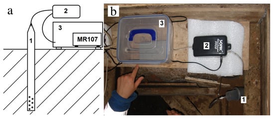
Figure 1.
Block diagram (a) and general view (b) of the subsoil radon registration kit: (1) perforated pipe in a borehole; (2) compressor; (3) accumulation chamber with the MR107 device.
The proposed measurement technique with subsoil air pumping out of the measuring borehole can significantly reduce the level of interference associated with variations in meteorological values: air temperature, atmospheric pressure and soil moisture [52].
The data obtained at several points of the network were used in the work, the description of which is given below. The location of the subsoil gas monitoring network points in Kamchatka was confined to the river valleys that trace the fault zones. Zones of dynamic fault influence have increased permeability, which contributes to the flow of subsoil gases into the atmosphere [1,53]. The points were located in different structural elements of the Avacha Bay coast [11,33].
One of the most equipped stations is the PRTR station, Figure 2.
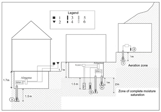
Figure 2.
Layout of sensors for recording the concentration of subsoil gases at the PRTR reference point. The numbers in the circles number the gas discharge meters: (1) pressure sensor; (2) temperature sensor; (3) gas-discharge counters -radiation; (4) sensor radiation; (5) molecular hydrogen sensor; (6) carbon dioxide sensor.
It is located on the river terrace of the Korkin stream, which traces the sublatitudinal fault within the Paratunka graben, with the hydrothermal system of the same name confined to it. At a distance of ≈700 m from the PRTR point downstream of the stream, there are natural outlets of thermal waters with a dissolved Rn content of up to [kBq/m]. Sensors for recording the concentration of subsoil gases (12 in total) at this point are located at 3 points along the profile perpendicular to the zone of dynamic influence of the fault Figure 2. Here, simultaneously with the counting of pulses from gas-discharge counters (depths up to 4 m from the daylight surface), the concentrations of carbon dioxide () and molecular hydrogen () are recorded. Registration on all sensors is carried out with a discreteness of 10 min.
Further, in the study from the PRTR point, the data of radon accumulation in the chamber where the sensor is installed are used, shown in Figure 3, averaged up to 1 h in the range for 6 intervals of 10 min.
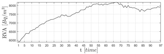
Figure 3.
Observation data from the PRTR observation point.
The YSSR site is located on the territory of the Sakhalin Branch of the “Unified Geophysical Service of the Russian Academy of Sciences” on the slope of a hill in the area of the YSS seismic station. It is equipped with a recording complex for continuous monitoring of radon in the subsoil air based on the RADEX MR107 radiometer. Subsurface air is pumped out from a depth of two meters [54,55]. Data in Figure 4 for RVA comparison were recorded in 30 min increments over 160 h.
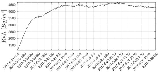
Figure 4.
Observation data from the YSSR observation point.
Data in Figure 5 show RVA obtained from the radon observation point GLLR located in the area of the Blue Lagoon basin in the area of the Paratunka hydrothermal system. Registration of the SAR was carried out in storage chambers at depths of 1 and 2 m, with a step of 2 min, for 22 h. The point is currently closed.
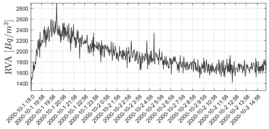
Figure 5.
Observation data from the GLLR observation point.
The MRZR point is located at the base of the Moroznaya-1 well (Yelizovsky district). The SBM-19 sensor was used in the storage chamber (standard bucket as before). At the point, RVA registration is carried out in storage chambers at depths of 0.2 and 1.0 m, with a step of 10 min for 96 h, as shown in Figure 6. This point was created to expand the network of monitoring subsoil gases and to find a connection between variations in the level of groundwater and the concentration of subsoil Rn, since the water level in the well is being recorded at this well.
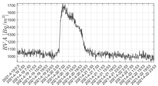
Figure 6.
Observation data from the MRZR observation point.
6. Simulation Results
Example 1.
Classical accumulation model RVA (1). Parameters , , .
Remark 15.
In the classical model, we can put , because RVA monitoring data will always be normalized to the maximum for comparison with model data.
Let us select RVA observational data, as in Figure 3 from the sensor at the PRTR point, which will be normalized to the maximum. Simulation results were not normalized, and both data types are represented by in relative units.
Carrying out the simulation according to the classical model (2) and comparing it with the experimental data from Figure 3, we obtain the calculated curves in Figure 7. Due to the properties of the solution to the Cauchy problem (1), it follows that it monotonically increases until saturation is reached, i.e., is capable of simulating only modes with saturation. The classical model (1) has only one control parameter—.
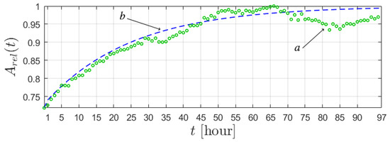
Example 2.
Hereditary α-model of RVA. Model parameter: , , , , .
To compare with the data in the YSSR item, as in Figure 4, the following actions will be performed: smoothing using the simple moving average [56,57] method with a window of three values and normalization to the maximum value. Simulation results were not normalized, and both types of data are presented in —relative units.
The values of the , parameters will be refined based on the normalized RVA data. The values , were chosen so that the solution (9) of the (8) model would give the maximum value of the Pearson correlation coefficient () [58] with normalized data YSSR observations. Note that this principle will continue to be observed.
Remark 16.
Due to the transition from integer to fractional derivative (6), a new parameter appears in the RVA hereditary α-model—the order of the fractional derivative α.
It can be seen from Figure 8 that for different values of , the RVA curves reach different levels of saturation. This is due to the fact that the parameter is responsible for the transfer intensity Rn. It can be seen from (Figure 8, –) that the smaller is, the lower the saturation level that RVA will reach, i.e., the RVA saturating process becomes slow. At , the permeability of the geo-environment decreases, and at , the permeability of the medium increases.
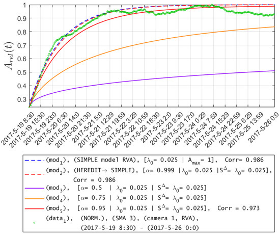
Figure 8.
Data on the accumulations of radon in the chamber on YSSR (green circle) and model curves with different parameters.
In the case of (9), with , we obtain a model curve almost similar to the (2) solution of the (1) classical model as shown in (Figure 8, – ). This confirms the correctness of the hereditary RVA model (7) on the example of the (8) model.
Example 3.
Hereditary α-model RVA (10). Model parameter: , , , , , , , .
For comparison, the following actions will be performed on the data from the sensor at the GLLR point in Figure 5: smoothing using the simple moving average [56,57] method with a window of four values and normalization to the maximum value. Simulation results were not normalized, and both types of data are presented in —relative units.
Function and constant parameters , were refined based on the RVA data so that the model solution would give the maximum value of the Pearson correlation coefficient () [58] and determination coefficient () [59,60] with normalized GLLR observational data.
From Figure 9, the best (red) calculated curve for the RVA hereditary model (10), with determination coefficients and correlation is shown in (Figure 9, ).
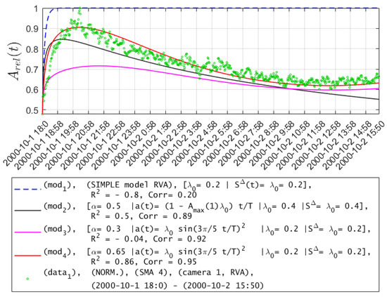
Figure 9.
Data on radon accumulation in the chamber on GLLR (green points) and model data with different model parameters.
Definition 6.
Using the nonlinear term in the RVA hereditary α-model (10), one can describe various dynamic RVA modes: a rapid increase in RVA values, then a slow decrease in RVA values, reaching some saturation. Quadratic nonlinearity is characteristic of the Riccati equation. In our case, we have a fractional Riccati equation, which was widely studied in [47,48].
Example 4.
Hereditary -RVA model (12). Model parameter: , , , , , , , .
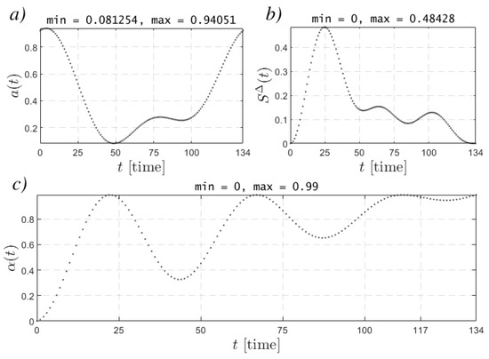
Figure 10.
Changing model parameters from time to time for Example 4.
The parameters of the , , , and functions were refined based on the processed RVA data. Periodic oscillations simulate changes in the permeability of the medium, deformation processes <<compression–stretch>>.
It can be seen from (Figure 7, Figure 8 and Figure 9) that the RVA data, as well as the model curves describing their saturation point, do not return to the initial level within the time interval of interest to us. However, sensors sometimes register sharp bursts of RVA in the storage chamber.
According to the RVA data, the surge in Figure 11 at the MRZR site resembles Rn injection in a water flow due to a change in the stress–strain state of the Earth’s crust. Figure 11 shows a sharp rise, and after a while a smoother decline in RVA, which may be accompanied by a slight increase in RVA values and further to the initial level, or close to the initial one. Further, in numerical experiments, for comparison with the results of mathematical modeling, we will use data describing only the RVA burst itself, as in Figure 11.
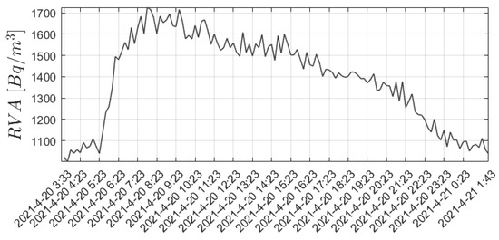
Figure 11.
Extracted from the data at the MRZR point Figure 6 burst RVA, lasting 22.5 h.
The following actions were performed on the data shown in Figure 11: smoothing using the <<Simple moving average>> [56,57] method with a window of two values; shifting to the minimum value; normalizing to the maximum value.
Definition 7.
The main difference of the RVA hereditary -model proposed here from the RVA hereditary α-model (10) is in the variable value of the order of the fractional derivative. Such a generalization enables us to model changes in the permeability of the geo-environment.
In Figure 12, at first, a sharp increase in RVA values is observed due to the intensification of Rn transfer under conditions of the stress–strain state of the geomedium. This is also reflected in the graphs of the function (Figure 10c) and (Figure 10b). As a result of compression of the geo-environment, Rn is squeezed out of pores and cracks, i.e., is ejected.
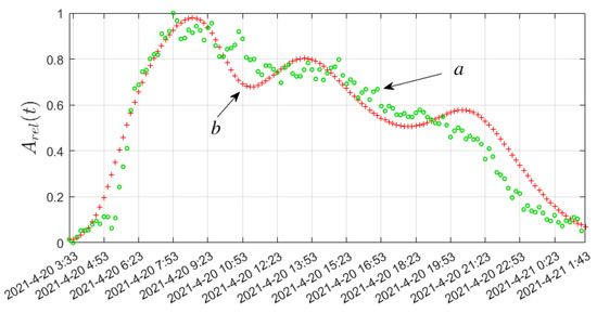
Figure 12.
(a) RVA burst data from MRZR in 10 min increments; (b) simulation results for (12) with determination coefficient () and Pearson correlation coefficient ().
It should be noted that the function , related to atmospheric pressure, decreases on the same time interval (Figure 10a). This also contributes to the growth of RVA values.
Further, we see that after some time (6 h,) the RVA values decrease. Such a decrease is noted in (Figure 10b) and (Figure 10c). This is due to the fact that the source of Rn emanation begins to dry up, and the process of transfer becomes less intense, perhaps the geo-environment is stretched. Mechanisms associated with meteorological conditions (atmospheric pressure) (Figure 10a), and air exchange with the atmosphere are included here. Further, we can observe minor bursts of RVA values, which are also associated with the stress–strain state of the geo-environment; however, the general trend towards a decrease in the level of Rn remains.
The memory effect (hereditarity) arising in the model due to the introduction of the fractional derivative is shown in (Figure 13a). This operator characterizes the rate of change in RVA and reflects the dissipation of RVA, as shown in (Figure 13b). Here we have some delay in time due to the memory effect of this dynamic system.
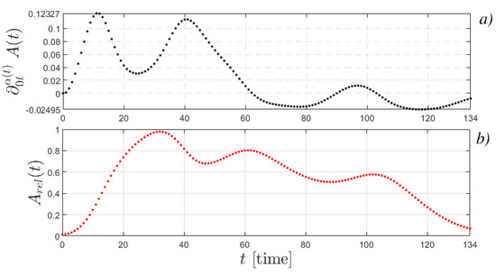
Figure 13.
Dependence in time: (a) on the value of the fractional derivative; (b) model curve (12) for Example 4.
7. Used Software
To solve the problems that arise during modeling, [41,48] used the developed software package, represented by the user library <<FDREext>> for the Maple 2021 symbolic mathematics environment. Earlier references [40] used an even earlier version of the custom library, namely <<FDRE 2.0>> for Maple 2021.
In this study, in order to simulate a dynamic process data processing, algorithms for numerical solution, and visualization of results, the software package <<FDRE 3.0>> in the MATLAB language was developed and a certificate of registration of computer programs No.2022668730 dated 10/11/2022 was obtained.
All results on the development, application, and verification of the proposed hereditary -model of RVA dynamics of Rn accumulation were obtained within the framework of the Russian Science Foundation grant No. 22-11-00064 on the topic “Modeling of dynamic processes in the geospheres taking into account heredity”.
This software package <<FDRE 3.0>> is a generalization of the ideas implemented earlier in <<FDREext>> and <<FDRE 2.0>> for solving problems and automating some actions that arise in the mathematical modeling of fractional dynamics processes. This software package is qualitatively different from previous developments, which is expressed in the following main qualities:
- Greater universality, as when working only with experimental data and modeling on them;
- Convenience of adding new variations of the model and experimental data for subsequent software processing;
- By orders of magnitude of increased speed, since it became possible to completely get away from symbolic calculations.
All visualizations in this article and related calculations of RVA models were performed in the developed software package <<FDRE 3.0>>.
8. Discussion
In the general case, variations in the RVA curves can be determined not only by changes in the stress state of the medium, and, consequently, by changes in its parameters, such as porosity, permeability, and fracturing. The concentration of radon in the subsoil air is quite strongly affected by atmospheric pressure, the temperature of the upper layer of soil and the air in it, soil moisture, and gusts of wind in the lower layer of the atmosphere.
The sharp rise in RVA is probably associated with deformations that cause changes in the flow of radon through the area under the accumulation chamber. In this case, the impact of a voltage pulse can be of different intensity and duration. As shown above, there are quite a lot of models describing radon migration in rocks. Based on them, it can be assumed that against the background of a constant flow of radon entering the chamber where the sensor is located, an excess volume of radon may occur, associated with a different reaction of the medium to deformation processes (according to the models from the works listed earlier). This excess radon, depending on the depth or volume of the environment in which it was released, enters the groundwater flow or new cracks that form and rushes to the surface of the Earth due to movement in the water flow, diffusion, and convection. This process determines the ascending part of the anomalous RVA curve relative to the background values. Since radon continuously decays after its formation, the maximum of the anomalous RVA curve is determined by the volume of released radon and the time of arrival from the depth where it began its migration.
The descending part on the graphs of anomalous RVA bursts in the accumulation chambers is associated with the decay of radon in the event that its excess supply to the chamber ceases. However, the graphs show that in most cases, the decrease in RVA occurs much faster than would be determined by the law of radioactive decay and the properties of radon. For example, in the case shown in Figure 12, the descending part of the anomalous curve is complicated by variations, and the entire anomaly returned to background values in less than a day, although in the case of a simple decay process of excess radon in the chamber, a return to doubled background values should have happened in about 4 days. What can be the reason for such a rapid decrease in radon in the accumulation chamber, as well as in some cases, variations in the RVA curve? The process leading to this can be a convective air flow through the accumulation chamber, which is associated with the heating of the upper soil layer, changes in atmospheric pressure at different periods, as well as gusts of wind, leading to the “spray” effect [11].
If the observed anomaly has a long duration, and the descending part of the curve develops within 3–10 days, then in this case the process of radioactive decay may prevail over the factors of change in the intensity of the convective component in the radon flow. The diffusion component in the radon flux is determined by the moisture saturation of the soil and the presence of open gas-filled pores and cracks and cannot increase rapidly.
Consequently, the processes that lead to the appearance of an excess volume of radon in the accumulation chamber can be associated with the expansion of the medium (an increase in free pores, the formation of new cracks, filling the pores with fluid and pushing gaseous radon to the surface), compression of the medium (squeezing out radon, increasing emanation due to excess energy due to heating of the medium from friction or desorption due to micro-oscillations, etc.), as well as with changes in the convective flow of subsoil air. At the same time, changes in the convective flow most intensively affect the shape of the curve, especially after the cessation of the entry of excess radon into the subsoil air.
9. Conclusions
The hereditary RVA -model and the RVA hereditary -model were used in this work to describe the dynamics of Rn accumulation taking into account the effect of heredity. The models were tested at Rn monitoring stations at the Petropavlovsk–Kamchatka geodynamic test site.
It is shown that the proposed models can describe not only the accumulation processes for a certain choice of parameters, but also the decay, as well as more complex impulses (bursts) of RVA due to the specific type of functions of the incoming model equations. This, in turn, can speak of the universality of the proposed models.
The work also gave an interpretation of the simulation results. It is shown that the order of the fractional derivative can be responsible for the intensity of the Rn transfer process (memory effect), which is associated with the permeability of the geo-environment: porosity, fracturing, etc. The nonlinear term in the model equations determines the Rn accumulation law close to the logistic one, which is described by the Riccati equation. Such nonlinearity gives a rapid increase in RVA values and saturation—some constant level.
Further development of the proposed models may consist of identifying the functions included in the model equations by solving the corresponding inverse problems.
It is also of interest to take into account deformations of the geomedium of various forms in the model equations, as by analogy with the work [21].
10. Patents
To simulate a dynamic process, data processing and algorithms for numerical solution and visualization of results, the <<FDRE 3.0>> software package in the MATLAB language was developed and a certificate of registration of computer programs No. 2022668730 dated 11 October 2022 was received.
Author Contributions
Conceptualization, D.T. and E.M.; methodology, E.M.; software, D.T.; validation, D.T.; formal analysis, E.M. and R.P.; investigation, D.T.; resources, E.M.; data curation, E.M.; writing—original draft preparation, D.T. and E.M.; writing—review and editing, R.P.; visualization, D.T.; supervision, R.P.; project administration, D.T.; funding acquisition, R.P. All authors have read and agreed to the published version of the manuscript.
Funding
This research was funded by Russian Science Foundation grant number 22-11-00064 «Modeling of dynamic processes in geospheres taking into account hereditarity» https://rscf.ru/project/22-11-00064/, accessed on 12 May 2022.
Data Availability Statement
Not applicable.
Conflicts of Interest
The authors declare no conflict of interest.
Abbreviations
The following abbreviations are used in this manuscript:
| RVA | Radon Volumetric Activity |
| Rn | Radon |
| AER | Air Exchange Rate |
| IFDS | Implicit Finite-difference Method |
References
- Rudakov, V.P. Emanational Monitoring of Geoenvironments and Processes; Science World: Moscow, Russia, 2009; p. 175. (In Russian) [Google Scholar]
- Adushkin, V.V.; Spivak, A.A. Physical Fields in Near-Surface Geophysics; GEOS: Moscow, Russia, 2014; p. 360. (In Russian) [Google Scholar]
- Neri, M.; Giammanco, S.; Ferrera, E.; Patane, G.; Zanon, V. Spatial distribution of soil radon as a tool to recognize active faulting on an active volcano: The example of Mt. Etna (Italy). J. Environ. Radioact. 2011, 102, 863–870. [Google Scholar] [CrossRef] [PubMed]
- Barberio, M.D.; Gori, F.; Barbieri, M.; Billi, A.; Devoti, R.; Doglioni, C.; Petitta, M.; Riguzzi, F.; Rusi, S. Diurnal and Semidiurnal Cyclicity of Radon (222Rn) in Groundwater, Giardino Spring, Central Apennines, Italy. Water 2018, 10, 1276. [Google Scholar] [CrossRef]
- Imme, G.; Morelli, D. Radon as earthquake precursor. In Earthquake Research and Analysis—Statistical Studies, Observations and Planning; D’Amico, S., Ed.; IntechOpen: London, UK, 2012; pp. 143–160. [Google Scholar] [CrossRef]
- Hauksson, E. Radon content of groundwater as an earthquake precursor: Evaluation of worldwide data and physical basis. J. Geophys. Res. Solid Earth 1981, 86, 9397–9410. [Google Scholar] [CrossRef]
- Cicerone, R.D.; Ebel, J.E.; Beitton, J. A systematic compilation of earthquake precursors. Tectonophysics 2009, 476, 371–396. [Google Scholar] [CrossRef]
- Petraki, E.; Nikolopoulos, D.; Panagiotaras, D.; Cantzos, D.; Yannakopoulos, P.; Nomicos, C.; Stonham, J. Radon-222: A Potential Short-Term Earthquake Precursor. Earth Sci. Clim. Chang. 2015, 6, 282. [Google Scholar] [CrossRef]
- İnan, S.; Akgül, T.; Seyis, C.; Saatçılar, R.; Baykut, S.; Ergintav, S.; Baş, M. Geochemical monitoring in the Marmara region (NW Turkey): A search for precursors of seismic activity. J. Geophys. Res. Solid Earth 2008, 113, 1–15. [Google Scholar] [CrossRef]
- Baykara, O.; Inceoz, M.; Doğru, M.; Aksoy, E.; Külahcı, F. Soil radon monitoring and anomalies in East Anatolian fault system (Turkey). J. Radioanal. Nucl. Chem. 2009, 279, 159–164. [Google Scholar] [CrossRef]
- Firstov, P.P.; Makarov, E.O.; Gluhova, I.P.; Budilov, D.I.; Isakevich, D.V. Search for predictive anomalies of strong earthquakes according to monitoring of subsoil gases at Petropavlovsk-Kamchatsky geodynamic test site. Geosystems Transit. Zones 2018, 2, 16–32. [Google Scholar] [CrossRef]
- Biryulin, S.V.; Kozlova, I.A.; Yurkov, A.K. Investigation of informative value of volume radon activity in soil during both the stress build up and tectonic earthquakes in the South Kuril region. Bull. KRASEC. Phys. Math. Sci. 2018, 4, 73–83. (In Russian) [Google Scholar] [CrossRef]
- Iwata, D.; Nagahama, H.; Muto, J.; Yasuoka, Y. Non-parametric detection of atmospheric radon concentration anomalies related to earthquakes. Sci. Rep. 2018, 8, 13028. [Google Scholar] [CrossRef]
- Parovik, R.I. Mathematical Modeling of the Non-Classical Theory of the Emanation Method; Vitus Bering Kamchatka State University: Petropavlovsk-Kamchatsky, Russia, 2014; p. 80. (In Russian) [Google Scholar]
- Wakita, H. Precursory Changes in Groundwater Prior to the 1978 Izu-Oshima-Kinkai Earthquake. In Earthquake Prediction: An International Review; Simpson, D.W., Richards, P.G., Eds.; American Geophysical Union: Washington, DC, USA, 1981; pp. 527–532. [Google Scholar] [CrossRef]
- Majumdar, K. A study of fluctuation in radon concentration behaviour as an earthquake precursor. Curr. Sci. 2004, 86, 1288–1292. [Google Scholar]
- Tsunomori, F.; Tanaka, H.; Murakami, M.; Tasaka, S. Seismic response of dissolved gas in groundwater. In Proceedings of the Workshop on Hydrological and Geochemical Research for Earthquake Prediction, Tsukuba, Taiwan, 25 November 2011; pp. 29–35. [Google Scholar]
- Kilbas, A.A.; Srivastava, H.M.; Trujillo, J.J. Theory and Applications of Fractional Differential Equations; Elsevier: Amsterdam, The Netherlands, 2006; p. 523. [Google Scholar]
- Nahushev, A.M. Fractional Calculus and Its Application; Fizmatlit: Moscow, Russia, 2003; p. 272. (In Russian) [Google Scholar]
- Uchaikin, V.V. Fractional Derivatives for Physicists and Engineers. Vol. I. Background and Theory; Springer: Berlin, Germany, 2013; p. 373. [Google Scholar] [CrossRef]
- Dubinchuk, V.T. Radon as a precursor of earthquakes. In Isotopic Geochemical Precursors of Earthquakes and Volcanic Eruption, Proceedings of the Advisory Group Meeting, Vienna, Austria, 9–12 September 1991; IAEA: Vienna, Austria, 1993; pp. 9–22. [Google Scholar]
- Gudzenko, V.V.; Dubinchuk, V.T. Isotopes of Radium and Radon in Natural Waters; Science: Moscow, Russia, 1987; p. 156. (In Russian) [Google Scholar]
- Gorbushina, L.V. Emanation method of indication of geodynamic processes in engineering-geological surveys. Sov. Geol. 1975, 4, 48–50. (In Russian) [Google Scholar] [CrossRef]
- King, C.Y. Gas-geochemical approaches to earthquake prediction. In Isotopic Geochemical Precursors of Earthquakes and Volcanic Eruption, Proceedings of the Advisory Group Meeting, Vienna, Austria, 9–12 September 1991; IAEA: Vienna, Austria, 1993; pp. 22–36. [Google Scholar]
- Kozlova, I.A.; Yurkov, A.K. Reflection of successive seismic events in the field of volumetric activity of radon. Ural Geophys. Bull. 1975, 27, 35–39. (In Russian) [Google Scholar]
- Barsukov, V.L.; Varshal, G.M.; Garanin, A.V.; Zamokina, N.S. Significance of hydrogeochemical methods for short-term earthquake prediction. In Hydrogeochemical Precursors of Earthquakes; Varshal, G.M., Ed.; Science: Moscow, Russia, 1985; pp. 3–16. (In Russian) [Google Scholar]
- Ponamarev, A.S. Fractionation in hydrothermal fluid as a potential opportunity for the formation of earthquake precursors. Geochemistry 1989, 5, 714–724. (In Russian) [Google Scholar]
- Varhegyi, A.; Baranyi, I.; Somogyi, G.A. Model for the vertical subsurface radon transport in «geogas» microbubbles. Geophys. Trans. 1986, 32, 235–253. [Google Scholar]
- Bondarenko, V.M.; Ivanova, T.M. Radon transport in a mountain range: Models and experimental data. Article I. Proc. High. Educ. Establ. Geol. Explor. 1999, 4, 96–107. (In Russian) [Google Scholar]
- Bondarenko, V.M.; Ivanova, T.M. Radon transport in a mountain range: Models and experimental data. Article II. Proc. High. Educ. Establ. Geol. Explor. 1999, 5, 108–115. (In Russian) [Google Scholar]
- Etiope, G.; Martinelli, G. Migration of carrier and trace gases in the geosphere: An overview. Phys. Earth Planet. Inter. 2002, 129, 185–204. [Google Scholar] [CrossRef]
- Novikov, G.F. Radiometric Intelligence; Science: Leningrad, Russia, 1989; p. 407. (In Russian) [Google Scholar]
- Firstov, P.P.; Makarov, E.O. Dynamics of Subsoil Radon in Kamchatka and Strong Earthquakes; Vitus Bering Kamchatka State University: Petropavlovsk-Kamchatsky, Russia, 2018; p. 148. (In Russian) [Google Scholar]
- Vasilyev, A.V.; Zhukovsky, M.V. Determination of mechanisms and parameters which affect radon entry into a room. J. Environ. Radioact. 2008, 1240, 185–190. [Google Scholar] [CrossRef]
- Parovik, R.I.; Shevtsov, B.M. Radon transfer processes in fractional structure medium. Math. Model. Comput. Simul. 2010, 2, 180–185. [Google Scholar] [CrossRef]
- Volterra, V. Functional Theory, Integral and Integro-Differential Equations; Blackie & Son Limited: London, UK, 1930; p. 226. [Google Scholar]
- Pskhu, A.V. Fractional Partial Differential Equations; Science: Moscow, Russia, 2005; p. 199. (In Russian) [Google Scholar]
- Gerasimov, A.N. Generalization of linear deformation laws and their application to internal friction problems. USSR Appl. Math. Mech. 1948, 12, 529–539. [Google Scholar]
- Caputo, M. Linear models of dissipation whose Q is almost frequency independent—II. Geophys. J. Int. 1946, 13, 529–539. [Google Scholar] [CrossRef]
- Tverdyi, D.A.; Parovik, R.I.; Makarov, E.O.; Firstov, P.P. Research of the process of radon accumulation in the accumulating chamber taking into account the nonlinearity of its entrance. E3S Web Conf. 2020, 196, 02027. [Google Scholar] [CrossRef]
- Tverdyi, D.A.; Parovik, R.I.; Makarov, E.O.; Firstov, P.P.; Alimova, N. Application of the Riccati hereditary mathematical model to the study of the dynamics of Radon accumulation in the storage chamber. EPJ Web Conf. 2021, 254, 03001. [Google Scholar] [CrossRef]
- Tvyordyj, D.A. Hereditary Riccati equation with fractional derivative of variable order. J. Math. Sci. 2021, 253, 564–572. [Google Scholar] [CrossRef]
- Rekhviashvili, S.S.; Pskhu, A.V. Fractional oscillator with exponential-power memory function. Lett. ZTF 2022, 48. [Google Scholar] [CrossRef]
- Patnaik, S.; Hollkamp, J.P.; Semperlotti, F. Applications of variable-order fractional operators: A review. Proc. R. Soc. A 2020, 476, 20190498. [Google Scholar] [CrossRef]
- Coimbra, C.F.M. Mechanics with variable-order differential operators. Annalen der Physik 2003, 12, 692–703. [Google Scholar] [CrossRef]
- Ortigueira, M.D.; Valerio, D.; Machado, J.T. Variable order fractional systems. Commun. Nonlinear Sci. Numer. Simul. 2019, 71, 231–243. [Google Scholar] [CrossRef]
- Tverdyi, D.A.; Parovik, R.I. Investigation of Finite-Difference Schemes for the Numerical Solution of a Fractional Nonlinear Equation. Fractal Fract. 2022, 6, 23. [Google Scholar] [CrossRef]
- Tverdyi, D.A.; Parovik, R.I. Application of the Fractional Riccati Equation for Mathematical Modeling of Dynamic Processes with Saturation and Memory Effect. Fractal Fract. 2022, 6, 163. [Google Scholar] [CrossRef]
- Rzkadkowski, G.; Sobczak, L. A generalized logistic function and its applications. Found. Manag. 2020, 12, 85–92. [Google Scholar] [CrossRef]
- Therese, A.S. Generalized Logistic Models. J. Am. Stat. Assoc. 1988, 83, 426–431. [Google Scholar] [CrossRef]
- Makarov, E.O.; Firstov, P.P.; Voloshin, V.N. Instrumental complex for registration concentration of subsurface gas to find precursory anomalies strong earthquake of Southern Kamchatka. Seism. Instrum. 2012, 48, 5–14. [Google Scholar]
- Utkin, V.I.; Yurkov, A.K. Radon as a tracer of tectonic movements. Geol. Geophys. 2010, 51, 277–286. [Google Scholar] [CrossRef]
- Firstov, P.P.; Rudakov, V.P. Results of registration of subsoil radon in 1997–2000 at the Petropavlovsk-Kamchatsky geodynamic test site. Volcanol. Seismol. 2019, 1, 26–41. (In Russian) [Google Scholar]
- Makarov, E.O.; Firstov, P.P.; Kostylev, D.V.; Rylov, E.S.; Dudchenko, I.P. Test mode of operation network of monitoring subsoil radon in the south of Sakhalin. E3S Web Conf. 2018, 62, 03007. [Google Scholar] [CrossRef]
- Makarov, E.O.; Firstov, P.P.; Kostylev, D.V.; Rylov, E.S.; Dudchenko, I.P. First results of subsurface radon monitoring by network of points, operating in the test mode on the south of Sakhalin iseland. Bull. KRASEC Phys. Math. Sci. 2018, 5, 99–114. [Google Scholar] [CrossRef]
- Chou, Y. Statistical Analysis: With Business & Economic Applications; Rinehart & Winston: New York, NY, USA, 1975; p. 894. [Google Scholar]
- Johnston, F.R.; Boyl, J.E.; Meadows, M.; Shale, E. Some properties of a simple moving average when applied to forecasting a time series. J. Oper. Res. Soc. 1999, 50, 1267–1271. [Google Scholar] [CrossRef]
- Cox, DRHinkley, D.V. Theoretical Statistics, 1st ed.; Chapman & Hall/CRC: London, UK, 1979; p. 528. [Google Scholar]
- Hughes, A.J.; Grawoig, D.E. Statistics: A Foundation for Analysis; Addison Wesley: Boston, MA. USA, 1971; p. 525. [Google Scholar]
- Chicco, D.; Warrens, M.J.; Jurman, G. The coefficient of determination R-squared is more informative than SMAPE, MAE, MAPE, MSE and RMSE in regression analysis evaluation. PeerJ Comput. Sci. 2021, 299, e623. [Google Scholar] [CrossRef]


Disclaimer/Publisher’s Note: The statements, opinions and data contained in all publications are solely those of the individual author(s) and contributor(s) and not of MDPI and/or the editor(s). MDPI and/or the editor(s) disclaim responsibility for any injury to people or property resulting from any ideas, methods, instructions or products referred to in the content. |
© 2023 by the authors. Licensee MDPI, Basel, Switzerland. This article is an open access article distributed under the terms and conditions of the Creative Commons Attribution (CC BY) license (https://creativecommons.org/licenses/by/4.0/).