Article

Mixed-Delay-Dependent Augmented Functional for Synchronization of Uncertain Neutral-Type Neural Networks with Sampled-Data Control

1
School of Computer, Chengdu University, Chengdu 610106, China
2
School of Electronic Information and Electrical Engineering, Chengdu University, Chengdu 610106, China
3
Geomathematics Key Laboratory of Sichuan Province, Chengdu University of Technology, Chengdu 610059, China
*
Author to whom correspondence should be addressed.
Mathematics 2023, 11(4), 872; https://doi.org/10.3390/math11040872
Submission received: 13 January 2023 / Revised: 5 February 2023 / Accepted: 6 February 2023 / Published: 8 February 2023

Abstract

:
In this paper, the synchronization problem of uncertain neutral-type neural networks (NTNNs) with sampled-data control is investigated. First, a mixed-delay-dependent augmented Lyapunov–Krasovskii functional (LKF) is proposed, which not only considers the interaction between transmission delay and communication delay, but also takes the interconnected relationship between neutral delay and transmission delay into consideration. Then, a two-sided looped functional is also involved in the LKF, which effectively utilizes the information on the intervals [ t k , t ] , [ t k τ , t τ ] , [ t , t k + 1 ) , [ t τ , t k + 1 τ ) . Furthermore, based on the suitable LKF and a free-matrix-based integral inequality, two synchronization criteria via a sampled-data controller considering communication delay are derived in forms of linear matrix inequalities (LMIs). Finally, three numerical examples are carried out to confirm the validity of the proposed criteria.

1. Introduction

Neural networks (NNs) are classes of mathematical models which simulate the neural processing mechanism in the human brain. Over the past several decades, NNs have attracted widespread attention due to their potential applications in many areas, such as image and signal processing [1], pattern recognition [2], optimization problems [3], parallel computation [4] and so on. In such systems, time delays may be generated due to the limited switching speeds of amplifiers and the inherent communication time among neurons. They may negatively impact the NNs and cause various undesired dynamical phenomena, such as oscillation or instability. Therefore, it is essential to consider time delays in the stability analysis of NNs.
Different forms of time delays have been conducted in the stability analysis of NNs, including variable delays [5], continuously distributed delays [6], and so on. In order to characterize the properties of neural reaction processes precisely, neutral-type time delays are involved in dynamical neural network models. In these models, the information about the derivative of the past state is considered. When both the current neuron state derivative and the past state derivative are involved in the NNs, neural network models are called neutral-type neural networks (NTNNs). Due to wide engineering applications in fields such as distributed networks [7], including lossless transmission lines [8] and heat exchangers [9], the stability and synchronization analysis of NTNNs having time delays and neutral delays has become an important research topic.
In recent years, various control methods have been brought to guarantee the synchronization of NTNNs. The sampled-data control method has been extensively applied due to its easy implementation [10,11]. This method can reduce network congestion and improve control efficiency. Three methods have been proposed to deal with the stability analysis of sampled-data control systems. The first one is the input delay method [12], where sampled-data systems are modeled as time-delay systems with a time-varying input. The second is the discrete-time method [13], in which sampled-data systems are transformed into discrete-time systems. However, this method suffers troubles when the sampling period is variable. The third method is the impulsive system method [14], which is often used to investigate systems with uncertain and bounded sampling intervals. Among these methods, the input delay method is widely used to investigate the synchronization of NTNNs with a sampled-data controller.
In addition, open communication networks are used in the control process. The communication delay is inevitably generated by the transmission of the signals from the sampler to the controller, and it may destabilize the sampled-data system. Therefore, it is crucial to design a sampled-data controller concerning communication delays. Recently, a new two-sided looped functional was proposed in [15], which can reduce conservativeness. However, only the information of intervals [ t k , t ] , [ t , t k + 1 ) is considered, while the information on the intervals [ t k τ c , t τ c ] , [ t τ c , t k + 1 τ c ) is ignored. In [16,17], the communication delays were considered in the design of the sampled-data controller, but some useful information about sample features is still lost. In [18,19], a mixed-delay-based LKF is proposed, and a less conservatism stability criterion is derived. Throughout analyzing these aspects, we find that a functional with more time-delay cross information can obtain better results than other functionals in the synchronization of NTNNs with sampled-data control.
Motivated by the above discussions, we further investigate the synchronization via sampled-data control for NTNNs with and without time-varying parameter uncertainties. The main contributions of this paper can be summarized as follows:
(i)
A sampled-data controller is designed considering the communication delay τ c . Such a method is easier to calculate and implement than the event-triggered communication scheme proposed in [20]. While guaranteeing system stability, this method can reduce network congestion and improve control efficiency.
(ii)
A mixed-delay-dependent augmented LKF is constructed. The interconnected relationship between transmission delay and communication delay is taken into account, and the interaction between transmission delay and neutral delay is considered simultaneously. This interconnected relationship is utilized by introducing some integral and double integral terms associated with the mixed delay. Thus, the connection between those states is strengthened.
(iii)
In order to reduce the conservatism of the synchronization criteria, a two-sided looped LKF is proposed, which utilizes the information of intervals [ t k , t ] , [ t k τ c , t τ c ] , [ t , t k + 1 ) , [ t τ c , t k + 1 τ c ) . This functional can obtain better results for sampled-data synchronization problems in NTNNs. Two less conservative synchronization criteria are derived based on the LKF and a free-matrix-based integral inequality.
N o t a t i o n s : Throughout this paper, N + represents the set of positive integers; R n denotes the n-dimensional vector space; the superscript 1 and T stand for the inverse and the transpose, respectively; P > 0 ( P 0 ) means that P is a positive definite matrix; I and 0 denote the identity matrix and a zero matrix, respectively; diag { x 1 , , x n } represents a diagonal matrix, in which its diagonal elements are x 1 , , x n , col { x 1 , , x n } = [ x 1 T , , x n T ] T and Sym { Z } = Z + Z T ; and the notation * stands for the symmetric terms in a symmetric matrix.

2. Preliminaries

In this section, we consider the following NTNNs with time-varying parameter uncertainties:
y ˙ ( t ) = ( A + Δ A ( t ) ) y ( t ) + ( W 0 + Δ W 0 ( t ) ) g ( y ( t ) ) + ( W 1 + Δ W 1 ( t ) ) g ( y ( t τ 2 ( t ) ) ) + ( W 2 + Δ W 2 ( t ) ) y ˙ ( t τ 1 ( t ) ) + J ,
where y ( · ) = col y 1 ( · ) , y 2 ( · ) , , y n ( · ) R n is the state vector with n neurons, A = diag { a 1 , a 2 , , a n } is a diagonal matrix with each a i > 0 ( i = 1 , 2 , , n ) , g ( y ( t ) ) = col g 1 ( y 1 ( t ) ) , g 2 ( y 2 ( t ) ) , , g n ( y n ( t ) ) R n is the neural activation function indicating how the neuron responses to its input, W 0 , W 1 and W 2 are the delayed interconnection weight matrices of appropriate dimensions, Δ A , Δ W 0 , Δ W 1 and Δ W 2 are parameter uncertainties, J = diag { J 1 , J 2 , , J n } is an external constant input vector.
τ 1 ( t ) stands for the neutral-type time delay, τ 2 ( t ) is the transmission delay accumulated during the transmission of information among neurons, which satisfy
0 τ i ( t ) τ i , τ ˙ i ( t ) μ i , i = 1 , 2 ,
where τ i and μ i are known positive constants.
The neuron activation function g ( · ) is bounded by
k i g i u 1 g i u 2 u 1 u 2 k i + , i = 1 , 2 , , n ,
where u 1 , u 2 R , u 1 u 2 , k i and k i + are real scalars. For convenience, define K + = diag { k 1 + , k 2 + , , k n + } , K = diag { k 1 , k 2 , , k n } .
Δ A ( t ) , Δ W 0 ( t ) , Δ W 1 ( t ) , Δ W 2 ( t ) are unknown matrices representing time-varying parameter uncertainties, which are assumed to be norm-bounded and satisfy
[ Δ A ( t ) Δ W 0 ( t ) Δ W 1 ( t ) Δ W 2 ( t ) ] = F Σ ( t ) [ E 1 E 2 E 3 E 4 ] , Σ ( t ) = Δ ( t ) [ I G Δ ( t ) ] 1 , I G T G > 0 ,
in which F and E i ( i = 1 , 2 , 3 , 4 ) are known constant matrices, Δ ( t ) is an unknown time-varying matrix satisfying Δ T ( t ) Δ ( t ) I .
Regarding system (1) as a master system, then, the corresponding slave system is described as follows:
z ˙ ( t ) = ( A + Δ A ( t ) ) z ( t ) + ( W 0 + Δ W 0 ( t ) ) g ( z ( t ) ) + ( W 1 + Δ W 1 ( t ) ) g ( z ( t τ 2 ( t ) ) ) + ( W 2 + Δ W 2 ( t ) ) z ˙ ( t τ 1 ( t ) ) + u ( t ) + J ,
where z ( · ) = col z 1 ( · ) , z 2 ( · ) , , z n ( · ) R n is the neural state and u ( t ) is the control input. The rest of the matrices and variables are defined in (1).
Define the error state as e ( t ) = z ( t ) y ( t ) , and thus, the error system is obtained as follows:
e ˙ ( t ) = ( A + Δ A ( t ) ) e ( t ) + ( W 0 + Δ W 0 ( t ) ) f ( e ( t ) ) + ( W 1 + Δ W 1 ( t ) ) f ( e ( t τ 2 ( t ) ) ) + ( W 2 + Δ W 2 ( t ) ) e ˙ ( t τ 1 ( t ) ) ) + u ( t ) ,
where f ( e ( t ) ) = g ( z ( t ) ) g ( y ( t ) ) satisfies
k i f i β β = g i e i + y i g i y i e i k i + , f i ( 0 ) = 0 , i = 1 , 2 , , n ,
where β R , β 0 .
Denote the updating instant time of the zero-order-hold (ZOH) by t k , e ( t k ) is the discrete measurements of e ( t ) at the sampling instant t k . For any integer k 0 , the sampling intervals are denoted by d k , which satisfy
d k = t k + 1 t k , d k ( 0 , d M ] ,
where d M > 0 stands for the upper bound of sampling intervals.
In practical systems, communication delays are inevitable during the transmission of signals from sampler to controller. Therefore, the communication delay τ c is considered in the sampled-data controller. Then, the control input u ( t ) is formulated as
u ( t ) = K e ( t k τ c ) , t [ t k , t k + 1 ) ,
where K is the controller gain matrix to be calculated.
For simplicity, we use η k to represent d k + τ c , where η k ( τ c , η M ] , η M = d M + τ c equals to the upper bound of η k .
Substituting the control input (9) into the error system (6), the corresponding error system can be reformulated as
e ˙ ( t ) = ( A + Δ A ( t ) ) e ( t ) + ( W 0 + Δ W 0 ( t ) ) f ( e ( t ) ) + ( W 1 + Δ W 1 ( t ) ) f ( e ( t τ 2 ( t ) ) ) + ( W 2 + Δ W 2 ( t ) ) e ˙ ( t τ 1 ( t ) ) ) + K e ( t k τ c ) .
In order to derive the stability criteria for the system (10), the following lemmas will be utilized.
Lemma 1 
([21]). Let x be a differentiable function: [ α , β ] R n . For symmetric matrices R > 0 , and N 1 , N 2 , N 3 , the following inequality holds:
α β x ˙ T ( s ) R x ˙ ( s ) d s ξ i T Ω i ξ i , i = 1 , 2 ,
where
Ω i = ( β α ) N 1 R 1 N 1 T + 1 3 N 2 R 1 N 2 T + 1 5 N 3 R 1 N 3 T + Sym N 1 Π 1 + N 2 Π 2 + N 3 Π 3 ( i ) , Π 1 = e ¯ 1 e ¯ 2 , Π 2 = e ¯ 1 + e ¯ 2 2 e ¯ 3 , Π 3 ( 1 ) = e ¯ 1 e ¯ 2 6 e ¯ 3 + 6 e ¯ 4 , Π 3 ( 2 ) = e ¯ 1 e ¯ 2 + 6 e ¯ 3 6 e ¯ 4 , ξ 1 = col x ( β ) , x ( α ) , 1 β α α β x ( s ) d s , 2 ( β α ) 2 α β α s x ( u ) d u d s , ξ 2 = col x ( β ) , x ( α ) , 1 β α α β x ( s ) d s , 2 ( β α ) 2 α β s β x ( u ) d u d s , e ¯ j = 0 n × ( j 1 ) n I n 0 n × ( 4 j ) n , j = 1 , 2 , , 4 .
Lemma 2 
([22]). Letting I G T G > 0 , define the set Υ = Δ ( t ) = Σ ( t ) [ I G Σ ( t ) ] 1 , Σ T ( t ) Σ ( t ) I and for given matrices H, Q and R of appropriate dimensions with H symmetrical, then H + Q Δ ( t ) R + R T Δ T ( t ) Q T < 0 , if and only if there exists a scalar δ > 0 such that
H R T δ Q * δ I δ G * * δ I = H + δ R δ 1 Q T T I G G T I 1 δ R δ 1 Q T < 0 .

3. Main Results

In this section, we will demonstrate the asymptotic stability of the NTNNs synchronization error system by constructing an augmented functional with mixed delays and a two-side looped functional. First, we take up the case Δ A ( t ) = Δ W 0 ( t ) = Δ W 1 ( t ) = Δ W 2 ( t ) = 0 .
Theorem 1. 
Given scalars ϵ 1 and ϵ 2 , if there exist symmetric matrices P i > 0 ( i = 1 , 2 , 3 ) , X j > 0 ( j = 1 , 2 , , 6 ) , S 1 > 0 , S 2 > 0 , Z 1 > 0 , Z 3 > 0 , R 2 > 0 , R 4 > 0 , Z 2 , Q 3 , Q 4 , R 1 , R 3 , any matrices Q 1 , Q 2 , G , L , Y k ( k = 1 , 2 , , 19 ) and diagonal matrices U 0 , V 0 , Δ l = d i a g λ l 1 , λ l 1 , , λ l n 0 ( l = 1 , 2 ) , such that the followed linear matrix inequalities (LMIs) hold:
Z 3 + R 1 > 0 , Z 2 + R 3 > 0 , Z 2 + Z 3 > 0 ,
Γ 1 + d k Γ 2 d k Θ 1 τ c Θ 2 τ 2 Θ 4 τ 1 Π T Y 18 τ 21 Π T Y 19 * χ 1 0 0 0 0 * * χ 2 0 0 0 * * * χ 4 0 0 * * * * S 1 0 * * * * * X 5 < 0 ,
Γ 1 + d k Γ 3 d k Θ 3 τ c Θ 2 τ 2 Θ 4 τ 1 Π T Y 18 τ 21 Π T Y 19 * χ 3 0 0 0 0 * * χ 2 0 0 0 * * * χ 4 0 0 * * * * S 1 0 * * * * * X 5 < 0 ,
where
Γ 1 = Sym Ω 1 T P 1 Ω 2 + ( r 11 K p r 1 ) T Δ 1 r 8 + ( K m r 1 r 11 ) T Δ 2 r 8 + Ω 9 T ( Q 1 Ω 10 + Q 2 Ω 11 ) + Ω 20 T Ω 21 + Ω 22 T U Ω 23 + Ω 24 T V Ω 25 + Ω 9 T ( Q 1 Ω 10 + Q 2 Ω 11 ) + Sym i = 1 19 Y i i + Ω 3 T P 2 Ω 3 ( 1 u 2 ) Ω 4 T P 2 Ω 4 + r 8 T P 3 r 8 ( 1 u 1 ) r 26 T P 3 r 26 + Ω 5 T ( X 1 + X 2 + X 3 ) Ω 5 Ω 6 T X 1 Ω 6 Ω 7 T X 2 Ω 7 Ω 8 T X 3 Ω 8 + r 24 T X 4 r 24 r 11 T X 4 r 11 + τ 21 r 8 T X 5 r 8 + r 11 T X 6 r 11 r 2 T X 6 r 2 + τ 1 r 8 T S 1 r 8 + τ 2 r 8 T S 2 r 8 + τ c r 8 T Z 1 r 8 + d M r 8 T Z 2 r 8 + η M r 8 T Z 3 r 8 , Γ 2 = Sym Ω 12 T ( Q 1 Ω 10 + Q 2 Ω 11 ) + Ω 13 T Q 1 Ω 14 + Ω 17 T Q 4 Ω 18 + Ω 11 T Q 3 Ω 11 + Ω 17 T Q 4 Ω 17 + r 8 T R 1 r 8 + r 9 T R 3 r 9 , Γ 3 = Sym Ω 15 T ( Q 1 Ω 10 + Q 2 Ω 11 ) + Ω 16 T Q 1 Ω 14 + Ω 17 T Q 4 Ω 19 Ω 11 T Q 3 Ω 11 Ω 17 T Q 4 Ω 17 + r 8 T R 2 r 8 + r 9 T R 4 r 9 , Γ 4 = τ c i = 1 3 1 2 i 1 Π T Y i Z 1 1 Y i T Π + τ c Π T Y 14 Z 3 1 Y 14 T Π + τ 2 i = 1 2 1 2 i 1 Π T Y 15 + i S 2 1 Y 15 + i T Π + τ 1 Π T Y 18 S 1 1 Y 18 T Π + τ 21 Π T Y 19 X 5 1 Y 19 T Π + i = 1 3 1 2 i 1 Π T Y 3 + i R 2 1 Y 3 + i T Π + i = 1 2 1 2 i 1 Π T Y 11 + i R 4 1 Y 11 + i T Π + Π T Y 15 ( Z 2 + Z 3 ) 1 Y 15 T Π , Γ 5 = τ c i = 1 3 1 2 i 1 Π T Y i Z 1 1 Y i T Π + τ c Π T Y 14 Z 3 1 Y 14 T Π + τ 2 i = 1 2 1 2 i 1 Π T Y 15 + i S 2 1 Y 15 + i T Π + τ 1 Π T Y 18 S 1 1 Y 18 T Π + τ 21 Π T Y 19 X 5 1 Y 19 T Π + i = 1 3 1 2 i 1 Π T Y 6 + i ( R 1 + Z 3 ) 1 Y 6 + i T Π + i = 1 2 1 2 i 1 Π T Y 9 + i ( R 3 + Z 2 ) 1 Y 9 + i T Π ,
τ 21 = τ 2 τ 1 , r i = 0 n × ( i 1 ) n I n 0 n × ( 26 i ) n , i = 1 , 2 , , 26 , Π = col r 1 , r 2 , r 3 , r 4 , r 5 , r 6 , r 7 , r 11 , r 15 , r 16 , r 17 , r 18 , r 19 , r 20 , r 21 , r 22 , r 23 , r 24 , Θ 1 = Π T Y 4 , Y 5 , Y 6 , Y 12 , Y 13 , Y 15 , Θ 2 = Π T Y 1 , Y 2 , Y 3 , Y 14 , Θ 3 = Π T Y 7 , Y 8 , Y 9 , Y 10 , Y 11 , Θ 4 = Π T Y 16 , Y 17 , χ 1 = diag R 2 , 3 R 2 , 5 R 2 , R 4 , 3 R 4 , Z 2 + Z 3 , χ 2 = diag Z 1 , 3 Z 1 , 5 Z 1 , Z 3 , χ 3 = diag R 1 + Z 3 , 3 ( R 1 + Z 3 ) , 5 ( R 1 + Z 3 ) , R 3 + Z 2 , 3 ( R 3 + Z 2 ) , χ 4 = diag S 2 , 3 S 2 , Ω 1 = col r 1 , r 2 , r 24 , r 11 , τ c r 15 τ 2 r 23 , τ c 2 r 16 , Ω 2 = col r 8 , r 9 , r 25 , r 10 , r 11 r 2 , τ c ( r 15 r 2 ) , Ω 3 = col r 1 , r 13 , Ω 4 = col r 12 , r 14 , Ω 5 = col r 1 , r 8 , Ω 6 = col r 11 , r 10 , Ω 7 = col r 2 , r 9 , Ω 8 = col r 24 , r 25 , Ω 9 = col r 3 r 1 , r 1 r 5 , r 4 r 2 , r 2 r 6 , Ω 10 = col r 1 r 3 , r 1 r 5 , r 2 r 4 , r 2 r 6 , Ω 11 = col r 3 , r 4 , r 5 , r 6 , Ω 12 = col r 8 , 0 , r 9 , 0 , Ω 13 = col r 1 r 3 , 0 , r 2 r 4 , 0 , Ω 14 = col r 8 , r 8 , r 9 , r 9 , Ω 15 = col 0 , r 8 , 0 , r 9 , Ω 16 = col 0 , r 1 r 5 , 0 , r 2 r 6 , Ω 17 = col r 17 , r 19 , r 21 , r 22 , r 18 , r 20 , Ω 18 = col r 1 r 17 , 0 , r 2 r 21 , 0 , r 17 2 r 18 , 0 , Ω 19 = col 0 , r 19 r 1 , 0 , r 22 r 2 , 0 , 2 r 20 r 19 , Ω 20 = col r 1 + ϵ 1 r 4 + ϵ 2 r 8 , Ω 21 = col G r 8 G A r 1 + G W 0 r 13 + G W 1 r 14 + G W 2 r 26 + L r 4 , Ω 22 = r 13 K r 1 , Ω 23 = K + r 1 r 13 , Ω 24 = r 14 K r 12 , Ω 25 = K + r 12 r 14 , 1 = r 1 r 2 , 2 = r 1 + r 2 2 r 15 , 3 = r 1 r 2 6 r 15 + 12 r 16 , 4 = r 5 r 1 , 5 = r 5 + r 1 2 r 19 , 6 = r 5 r 1 + 6 r 19 12 r 20 , 7 = r 1 r 3 , 8 = r 1 + r 3 2 r 17 , 9 = r 1 r 3 6 r 17 + 12 r 18 , 10 = r 2 r 4 , 11 = r 2 + r 4 2 r 21 , 12 = r 6 r 2 , 13 = r 6 + r 2 2 r 22 , 14 = r 3 r 4 , 15 = r 4 r 7 , 16 = r 1 r 11 , 17 = r 1 + r 11 2 r 23 , 18 = r 1 r 24 , 19 = r 24 r 11 .
Then, the slave system (5) can be synchronized with the master system (1). The gain matrix of the controller in (6) can be calculated by K = G 1 L .
Proof. 
Please see Appendix A.    □
Remark 1. 
The two-side looped functional W ( t ) was introduced in the LKF, which utilized the information on intervals [ t k , t ] , [ t k τ , t τ ] , [ t , t k + 1 ) , [ t τ , t k + 1 τ ) . Notice that W j ( t ) ( j = 1 , 2 , 3 , 4 , 5 ) satisfy the requirement of the looped functional [23] as follows: W j ( t k ) = W j ( t k + 1 ) = 0 .
Remark 2. 
Even though the existence of neutral delay τ 1 ( t ) and transmission delay τ 2 ( t ) were considered, the cross information associated with the states of the mixed delays were not exploited in [7,24,25]. In our work, the integral terms and double integral terms in V 4 ( t ) can reflect the cross information associated with the time delays τ i ( t ) ( i = 1 , 2 ) . The derivative of LKF conducted not only depends on τ i ( t ) ( i = 1 , 2 ) , but also on the value τ 21 . These integral terms strengthen the connection between those states and effectively reduce the conservatism when τ 1 ( t ) τ 2 ( t ) .
Remark 3. 
The sampling periods d k and the communication delay τ c are coupled with the variable matrices in LMIs. We set the communication delay τ c as a given scalar, and then use Algorithm 1 to derive the maximal sampling period d M and the corresponding controller gain K.
Algorithm 1 Find the maximum sampling period d M and the controller gain matrix K.
  • Step 1: Input communication delay τ c .
  • Step 2: Set the accuracy coefficient to d a c = 0.0001 , and initialize the search interval
  • d min , d max with d min = 0 and a large enough integer d max .
  • Step 3: By validating the feasibility of LMIs ( 14 ) and ( 15 ) , determine whether the
  •          system has a sampling period given as d t = d min + d max / 2 .
  • Step 4: If ( 14 ) and (15) are feasible, calculate K t by (A3), and set d min = d t ; else, set
  • d max = d t .
  • Step 5: If d max d min d a c , record the maximum sampling period d M = d min
  •          and derive the corresponding controller gain K = K t ; else, repeat Step 3.
  • Step 6: End. Output d M and K.
To demonstrate the validity of the mixed-delay-dependent terms in LKF, we remove them from Theorem 1, resulting in Corollary 1.
Corollary 1. 
Given scalars ϵ 1 and ϵ 2 , if there exist symmetric matrices P i > 0 ( i = 1 , 2 , 3 ) , X j > 0 ( j = 1 , 2 , , 6 ) , S 1 > 0 , S 2 > 0 , Z 1 > 0 , Z 3 > 0 , R 2 > 0 , R 4 > 0 , Z 2 , Q 3 , Q 4 , R 1 , R 3 , any matrices Q 1 , Q 2 , G , L , Y k ( k = 1 , 2 , , 18 ) and diagonal matrices U 0 , V 0 , Δ l = d i a g λ l 1 , λ l 1 , , λ l n 0 ( l = 1 , 2 ) , such that the followed linear matrix inequalities (LMIs) hold:
Z 3 + R 1 > 0 , Z 2 + R 3 > 0 , Z 2 + Z 3 > 0 ,
Γ ^ 1 + d k Γ 2 d k Θ 1 τ c Θ 2 τ 2 Θ 4 τ 1 Π T Y 18 * χ 1 0 0 0 * * χ 2 0 0 * * * χ 4 0 * * * * S 1 < 0 ,
Γ ^ 1 + d k Γ 3 d k Θ 3 τ c Θ 2 τ 2 Θ 4 τ 1 Π T Y 18 * χ 3 0 0 0 * * χ 2 0 0 * * * χ 4 0 * * * * S 1 < 0 ,
where
Γ ^ 1 = Sym r 1 T P 1 r 8 + ( r 11 K r 1 ) T Δ 1 r 8 + ( K + r 1 r 11 ) T Δ 2 r 8 + Ω 9 T ( Q 1 Ω 10 + Q 2 Ω 11 ) + Ω 20 T Ω 21 + Ω 22 T U Ω 23 + Ω 24 T V Ω 25 + Π 9 T ( Q 1 Π 10 + Q 2 Π 11 ) + Sym i = 1 18 Y i i + Ω 3 T P 2 Ω 3 ( 1 u 2 ) Ω 4 T P 2 Ω 4 + r 8 T P 3 r 8 ( 1 u 1 ) r 26 T P 3 r 26 + Ω 5 T ( X 1 + X 2 + X 3 ) Ω 5 Ω 6 T X 1 Ω 6 Ω 7 T X 2 Ω 7 Ω 8 T X 3 Ω 8 + τ 1 r 8 T S 1 r 8 + τ 2 r 8 T S 2 r 8 + τ c r 8 T Z 1 r 8 + d M r 8 T Z 2 r 8 + η M r 8 T Z 3 r 8 ,
and the rest of the vectors and matrices are defined in Theorem 1. Then, the slave system (5) can be synchronized with the master system (1). The gain matrix of the controller in (6) can be calculated by K = G 1 L .
Proof. 
Please see Appendix B. □
Remark 4. 
In Corollary 1, we remove the mixed-delay terms in V 4 ( t ) , and change the vector ϖ 1 ( t ) to e ( t ) . The comparison between Theorem 1 and Corollary 1 demonstrates the usefulness of the mixed-delay terms. Example 1 in Section 4 shows numerical comparisons.
Based on Theorem 1 and considering the parameter uncertainties, we have the following stability conditions.
Theorem 2. 
Given scalars ϵ 1 , ϵ 2 , matrices J , E m > 0 ( m = 1 , 2 , 3 , 4 ) , if there exist positive scalars δ n > 0 ( n = 1 , 2 ) , symmetric matrices P i > 0 ( i = 1 , 2 , 3 ) , X j > 0 ( j = 1 , 2 , , 6 ) , S 1 > 0 , S 2 > 0 , Z 1 > 0 , Z 3 > 0 , R 2 > 0 , R 4 > 0 , Z 2 , Q 3 , Q 4 , R 1 , R 3 , any matrices Q 1 , Q 2 , G , L , Y k ( k = 1 , 2 , , 19 ) and diagonal matrices U 0 , V 0 , Δ l = d i a g λ l 1 , λ l 1 , , λ l n 0 ( l = 1 , 2 ) , such that the following LMIs hold:
Z 3 + R 1 > 0 , Z 2 + R 3 > 0 , Z 2 + Z 3 > 0 ,
Γ 1 + d k Γ 2 d k Θ 1 τ c Θ 2 τ 2 Θ 4 τ 1 Y ˜ 18 τ 21 Y ˜ 19 δ 1 Ψ 1 Ψ 2 * χ 1 0 0 0 0 0 0 * * χ 2 0 0 0 0 0 * * * χ 4 0 0 0 0 * * * * S 1 0 0 0 * * * * * X 5 0 0 * * * * * * δ 1 I δ 1 J * * * * * * * δ 1 I < 0 ,
Γ 1 + d k Γ 3 d k Θ 3 τ c Θ 2 τ 2 Θ 4 τ 1 Y ˜ 18 τ 21 Y ˜ 19 δ 2 Ψ 1 Ψ 2 * χ 3 0 0 0 0 0 0 * * χ 2 0 0 0 0 0 * * * χ 4 0 0 0 0 * * * * S 1 0 0 0 * * * * * X 5 0 0 * * * * * * δ 2 I δ 2 J * * * * * * * δ 2 I < 0 ,
where Γ i , Θ i , χ i ( i = 1 , 2 , 3 , 4 ) are defined well in Theorem 1 and Y ˜ 18 = Π T Y 18 , Y ˜ 19 = Π T Y 19 , Ψ 1 = col E 1 T , 0 n · 11 n T , E 2 T , E 3 T , 0 n · 11 n T , E 4 T , Ψ 2 = col G F , 0 n · 2 n T , ϵ 1 G F , 0 n · 3 n T , ϵ 2 G F , 0 n · 18 n T . Then, the slave system (5) can be synchronized with the master system (1). The gain matrix of the controller in (6) can be calculated by K = G 1 L .
Proof. 
Please see Appendix C. □
To demonstrate the validity of the mixed-delay-dependent terms in LKF, we remove them from Theorem 2, resulting in Corollary 2.
Corollary 2. 
Given scalars ϵ 1 , ϵ 2 , matrices J , E m > 0 ( m = 1 , 2 , 3 , 4 ) , if there exist positive scalars δ n > 0 ( n = 1 , 2 ) , symmetric matrices P i > 0 ( i = 1 , 2 , 3 ) , X j > 0 ( j = 1 , 2 , , 6 ) , S 1 > 0 , S 2 > 0 , Z 1 > 0 , Z 3 > 0 , R 2 > 0 , R 4 > 0 , Z 2 , Q 3 , Q 4 , R 1 , R 3 , any matrices Q 1 , Q 2 , G , L , Y k ( k = 1 , 2 , , 18 ) and diagonal matrices U 0 , V 0 , Δ l = d i a g λ l 1 , λ l 1 , , λ l n 0 ( l = 1 , 2 ) , such that the following LMIs hold:
Z 3 + R 1 > 0 , Z 2 + R 3 > 0 , Z 2 + Z 3 > 0 ,
Γ ^ 1 + d k Γ 2 d k Θ 1 τ c Θ 2 τ 2 Θ 4 τ 1 Y ˜ 18 δ 1 Ψ 1 Ψ 2 * χ 1 0 0 0 0 0 * * χ 2 0 0 0 0 * * * χ 4 0 0 0 * * * * S 1 0 0 * * * * * δ 1 I δ 1 J * * * * * * δ 1 I < 0 ,
Γ ^ 1 + d k Γ 3 d k Θ 3 τ c Θ 2 τ 2 Θ 4 τ 1 Y ˜ 18 δ 2 Ψ 1 Ψ 2 * χ 3 0 0 0 0 0 * * χ 2 0 0 0 0 * * * χ 4 0 0 0 * * * * S 1 0 0 * * * * * δ 2 I δ 2 J * * * * * * δ 2 I < 0 ,
where
Γ ^ 1 = Sym r 1 T P 1 r 8 + ( r 11 K r 1 ) T Δ 1 r 8 + ( K + r 1 r 11 ) T Δ 2 r 8 + Ω 9 T ( Q 1 Ω 10 + Q 2 Ω 11 ) + Ω 20 T Ω 21 + Ω 22 T U Ω 23 + Ω 24 T V Ω 25 + Π 9 T ( Q 1 Π 10 + Q 2 Π 11 ) + Sym i = 1 18 Y i i + Ω 3 T P 2 Ω 3 ( 1 u 2 ) Ω 4 T P 2 Ω 4 + r 8 T P 3 r 8 ( 1 u 1 ) r 26 T P 3 r 26 + Ω 5 T ( X 1 + X 2 + X 3 ) Ω 5 Ω 6 T X 1 Ω 6 Ω 7 T X 2 Ω 7 Ω 8 T X 3 Ω 8 + τ 1 r 8 T S 1 r 8 + τ 2 r 8 T S 2 r 8 + τ c r 8 T Z 1 r 8 + d M r 8 T Z 2 r 8 + η M r 8 T Z 3 r 8 ,
and the rest of the vectors and matrices are defined in Theorem 2. Then, the slave system (5) can be synchronized with the master system (1). The gain matrix of the controller in (6) can be calculated by K = G 1 L .
Proof. 
Please see Appendix D. □
If the neutral delay is not taken into consideration, the following synchronization criterion is derived.
Corollary 3. 
Given scalars ϵ 1 and ϵ 2 , if there exist symmetric matrices P i > 0 ( i = 1 , 2 ) , X j > 0 ( j = 2 , 3 ) , S 1 > 0 , Z 1 > 0 , Z 3 > 0 , R 2 > 0 , R 4 > 0 , Z 2 , Q 3 , Q 4 , R 1 , R 3 , any matrices Q 1 , Q 2 , G , L , Y k ( k = 1 , 2 , , 17 ) and diagonal matrices U 0 , V 0 , Δ l = d i a g λ l 1 , λ l 1 , , λ l n 0 ( l = 1 , 2 ) , such that the following linear matrix inequalities (LMIs) hold:
Z 3 + R 1 > 0 , Z 2 + R 3 > 0 , Z 2 + Z 3 > 0 ,
Γ ˜ 1 + d k Γ ˜ 2 d k Θ ˜ 1 τ c Θ ˜ 2 τ 2 Θ ˜ 4 * χ 1 0 0 * * χ 2 0 * * * χ 4 < 0 ,
Γ ˜ 1 + d k Γ ˜ 3 d k Θ ˜ 3 τ c Θ ˜ 2 τ 2 Θ ˜ 4 * χ 3 0 0 * * χ 2 0 * * * χ 4 < 0 ,
where
Γ ˜ 1 = Sym Ω ˜ 1 T P 1 Ω ˜ 2 + ( r ˜ 11 K r ˜ 1 ) T Δ 1 r ˜ 8 + ( K + r ˜ 1 r ˜ 11 ) T Δ 2 r ˜ 8 + Ω ˜ 9 T ( Q 1 Ω ˜ 10 + Q 2 Ω ˜ 11 ) + Ω ˜ 20 T Ω ˜ 21 + Ω ˜ 22 T U Ω ˜ 23 + Ω ˜ 24 T V Ω ˜ 25 + Ω ˜ 9 T ( Q 1 Ω ˜ 10 + Q 2 Ω ˜ 11 ) + Sym i = 1 17 Y i ˜ i + Ω ˜ 3 T P 2 Ω ˜ 3 ( 1 u 2 ) Ω ˜ 4 T P 2 Ω ˜ 4 + Ω ˜ 5 T ( X 2 + X 3 ) Ω ˜ 5 Ω ˜ 7 T X 2 Ω ˜ 7 Ω ˜ 8 T X 3 Ω ˜ 8 + r ˜ 11 T X 6 r ˜ 11 r ˜ 2 T X 6 r ˜ 2 + τ 2 r ˜ 8 T S 1 r ˜ 8 + τ c r ˜ 8 T Z 1 r ˜ 8 + d M r ˜ 8 T Z 2 r ˜ 8 + η M r ˜ 8 T Z 3 r ˜ 8 ,
Γ ˜ 2 = Sym Ω ˜ 12 T ( Q 1 Ω ˜ 10 + Q 2 Ω ˜ 11 ) + Ω ˜ 13 T Q 1 Ω ˜ 14 + Ω ˜ 17 T Q 4 Ω ˜ 18 + Ω ˜ 11 T Q 3 Ω ˜ 11 + Ω ˜ 17 T Q 4 Ω ˜ 17 + r ˜ 8 T R 1 r ˜ 8 + r ˜ 9 T R 3 r ˜ 9 , Γ ˜ 3 = Sym Ω ˜ 15 T ( Q 1 Ω ˜ 10 + Q 2 Ω ˜ 11 ) + Ω ˜ 16 T Q 1 Ω ˜ 14 + Ω ˜ 17 T Q 4 Ω ˜ 19 Ω ˜ 11 T Q 3 Ω ˜ 11 Ω ˜ 17 T Q 4 Ω ˜ 17 + r ˜ 8 T R 2 r ˜ 8 + r ˜ 9 T R 4 r ˜ 9 , r ˜ i = 0 n × ( i 1 ) n I n 0 n × ( 23 i ) n , i = 1 , 2 , , 23 , Π ˜ = col r 1 , r 2 , r 3 , r 4 , r 5 , r 6 , r 7 , r 11 , r 15 , r 16 , r 17 , r 18 , r 19 , r 20 , r 21 , r 22 , r 23 , Θ ˜ 1 = Π ˜ T Y 4 , Y 5 , Y 6 , Y 12 , Y 13 , Y 15 , Θ ˜ 2 = Π ˜ T Y 1 , Y 2 , Y 3 , Y 14 , Θ ˜ 3 = Π ˜ T Y 7 , Y 8 , Y 9 , Y 10 , Y 11 , Θ ˜ 4 = Π ˜ T Y 16 , Y 17 , χ 1 = diag R 2 , 3 R 2 , 5 R 2 , R 4 , 3 R 4 , Z 2 + Z 3 , χ 2 = diag Z 1 , 3 Z 1 , 5 Z 1 , Z 3 , χ 3 = diag R 1 + Z 3 , 3 ( R 1 + Z 3 ) , 5 ( R 1 + Z 3 ) , R 3 + Z 2 , 3 ( R 3 + Z 2 ) , χ 4 = diag S 2 , 3 S 2 , Ω ˜ 1 = col r ˜ 1 , r ˜ 2 , r ˜ 11 , τ c r ˜ 15 τ 2 r ˜ 23 , τ c 2 r ˜ 16 , Ω ˜ 2 = col r ˜ 8 , r ˜ 9 , r ˜ 10 , r ˜ 11 r ˜ 2 , τ c ( r ˜ 15 r ˜ 2 ) , Ω ˜ 3 = col r ˜ 1 , r ˜ 13 , Ω ˜ 4 = col r ˜ 12 , r ˜ 14 , Ω ˜ 5 = col r ˜ 1 , r ˜ 8 , Ω ˜ 7 = col r ˜ 2 , r ˜ 9 , Ω ˜ 8 = col r ˜ 11 , r ˜ 10 , Ω ˜ 9 = col r ˜ 3 r ˜ 1 , r ˜ 1 r ˜ 5 , r ˜ 4 r ˜ 2 , r ˜ 2 r ˜ 6 , Ω ˜ 10 = col r ˜ 1 r ˜ 3 , r ˜ 1 r ˜ 5 , r ˜ 2 r ˜ 4 , r ˜ 2 r ˜ 6 , Ω ˜ 11 = col r ˜ 3 , r ˜ 4 , r ˜ 5 , r ˜ 6 , Ω ˜ 12 = col r ˜ 8 , 0 , r ˜ 9 , 0 , Ω ˜ 13 = col r ˜ 1 r ˜ 3 , 0 , r ˜ 2 r ˜ 4 , 0 , Ω ˜ 14 = col r ˜ 8 , r ˜ 8 , r ˜ 9 , r ˜ 9 , Ω ˜ 15 = col 0 , r ˜ 8 , 0 , r ˜ 9 , Ω ˜ 16 = col 0 , r ˜ 1 r ˜ 5 , 0 , r ˜ 2 r ˜ 6 , Ω ˜ 17 = col r ˜ 17 , r ˜ 19 , r ˜ 21 , r ˜ 22 , r ˜ 18 , r ˜ 20 , Ω ˜ 18 = col r ˜ 1 r ˜ 17 , 0 , r ˜ 2 r ˜ 21 , 0 , r ˜ 17 2 r ˜ 18 , 0 , Ω ˜ 19 = col 0 , r ˜ 19 r ˜ 1 , 0 , r ˜ 22 r ˜ 2 , 0 , 2 r ˜ 20 r ˜ 19 , Ω ˜ 20 = col r ˜ 1 + ϵ 1 r ˜ 4 + ϵ 2 r ˜ 8 , Ω ˜ 21 = col G r ˜ 8 G A r ˜ 1 + G W 0 r ˜ 13 + G W 1 r ˜ 14 + L r ˜ 4 , Ω ˜ 22 = r ˜ 13 K r ˜ 1 , Ω ˜ 23 = K + r ˜ 1 r ˜ 13 , Ω ˜ 24 = r ˜ 14 K r ˜ 12 , Ω ˜ 25 = K + r ˜ 12 r ˜ 14 , ˜ 1 = r ˜ 1 r ˜ 2 , ˜ 2 = r ˜ 1 + r ˜ 2 2 r ˜ 15 , ˜ 3 = r ˜ 1 r ˜ 2 6 r ˜ 15 + 12 r ˜ 16 , ˜ 4 = r ˜ 5 r ˜ 1 , ˜ 5 = r ˜ 5 + r ˜ 1 2 r ˜ 19 , ˜ 6 = r ˜ 5 r ˜ 1 + 6 r ˜ 19 12 r ˜ 20 , ˜ 7 = r ˜ 1 r ˜ 3 , ˜ 8 = r ˜ 1 + r ˜ 3 2 r ˜ 17 , ˜ 9 = r ˜ 1 r ˜ 3 6 r ˜ 17 + 12 r ˜ 18 , ˜ 10 = r ˜ 2 r ˜ 4 , ˜ 11 = r ˜ 2 + r ˜ 4 2 r ˜ 21 , ˜ 12 = r ˜ 6 r ˜ 2 , ˜ 13 = r ˜ 6 + r ˜ 2 2 r ˜ 22 , ˜ 14 = r ˜ 3 r ˜ 4 , ˜ 15 = r ˜ 4 r ˜ 7 , ˜ 16 = r ˜ 1 r ˜ 11 , ˜ 17 = r ˜ 1 + r ˜ 11 2 r ˜ 23 .
Then, the slave system can be synchronized with the master system. The gain matrix of the controller can be calculated by K = G 1 L .
Proof. 
Please see Appendix E. □

4. Illustrative Examples

In this section, three numerical examples will be presented to illustrate the validity of the derived criteria.
Example 1. 
Consider the neutral-type neural networks (10) with the following parameters [19]:
A = 3 0 0 3 , W 0 = 0.5 0.3 0.3 0.5 , W 1 = 0.2 0.1 0.1 0.2 , W 2 = 0.15 0 0 0.15 , K = diag 0 , 0 , K + = diag 1 , 1 , Δ A ( t ) = 0 , Δ W 0 ( t ) = 0 , Δ W 1 ( t ) = 0 , Δ W 2 ( t ) = 0 .
We choose τ 1 = 0.5 , μ 1 = 0.9 , τ 2 = 2.0 , μ 2 = 0.5 , ϵ 1 = ϵ 2 = 0.24 . For different communication delays τ c , via solving the LMIs in Theorem 1 and Corollary 1, the maximal sampling period d m computed by Algorithm 1 are listed in Table 1. It can be seen from Table 1 that as the communication delays τ c increases, the maximum sampling period d M decreases. Theorem 1 and Corollary 1 are derived via a similar approach. When τ c = 0.09 , the maximum sampling period d M calculated by Corollary 1 is 1.2996 and by Theorem 1 is 1.3738 . Theorem 1 provides a larger allowable sampling period than Corollary 1. Therefore, a mixed-delay-dependent LKF can lead to a less conservative result.
When τ c = 0.01 , d M = 1.3881 , the corresponding controller gain matrix is obtained by Theorem 1 as follows:
K = 0.0653 0.0414 0.0414 0.0653 .
Let τ c = 0.01 , the largest sampling interval d M = 1.3881 , and the corresponding controller is obtained as
K = 0.0653 0.0414 0.0414 0.0653 .
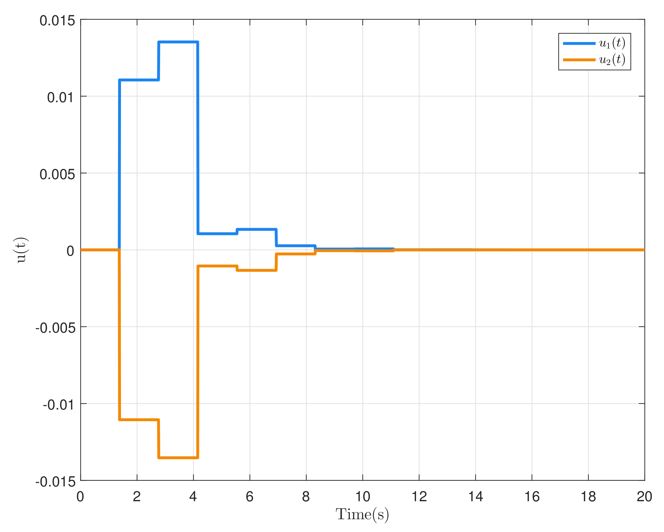
The neural activation function is taken as the form f i ( x i ) = t a n h ( x i ) ( i = 1 , 2 ) , which satisfies the assumption (7). The time-delay τ 1 ( t ) = 0.5 s i n 2 ( 0.9 t ) , and τ 2 ( t ) = 2 c o s 2 ( 0.5 t ) . The initial condition of the master system and the slave system are taken as x ( 0 ) = col { 0.2 , 0.3 } , y ( 0 ) = col { 0.3 , 0.6 } , respectively. The initial control input is u ( t ) = 0 . Let the sampling period d k = d M , based on the above sample-data controller, the state response of the error system (6) is shown in Figure 1, and the control input (9) is shown in Figure 2. It can be seen from Figure 1 that the error state converges to zero. That is to say, the error system (6) is asymptotic stable, and the slave system (5) is synchronous with the master system (1). It verifies the effectiveness of our methods.
Example 2. 
Consider the neutral-type neural networks (10) with the following parameters [19]:
A = diag 3 , 3 , K = diag 0 , 0 , K + = diag 1 , 1 , W 0 = 1 0.1 0.1 1 , W 1 = 0.4 0.1 0.04 0.1 , W 2 = 0.01 0 0 0.01 .
In this example, the time-varying parameter uncertainties Δ A ( t ) , Δ W 0 ( t ) , Δ W 1 ( t ) , Δ W 2 ( t ) are defined as [ Δ A ( t ) Δ W 0 ( t ) Δ W 1 ( t ) Δ W 2 ( t ) ] = F Σ ( t ) [ E 1 E 2 E 3 E 4 ] , where E 1 = [ 0.1 , 0.02 ] , E 2 = [ 0.07 , 0.1 ] , E 3 = [ 0.02 , 0.02 ] , E 4 = [ 0.01 , 0.02 ] , F = diag { 1 , 1 } , Σ ( t ) = s i n t . We choose τ 1 = 0.5 , μ 1 = 0.9 , μ 2 = 0.5 , τ 2 = 2 .
The maximum sampling period d M for different τ c by Theorem 2 is listed in Table 2. By solving the LMIs (19)–(21), Theorem 2 provides a larger allowable upper bound of delays than those in Corollary 2. That is to say, the LKF containing a mixed delay part can lead to a less conservative result effectively.
Based on Theorem 2, when τ c = 0.01 , the maximum sampling period d M = 26.2134 , the desired controller gain matrix can be calculated as
K = 0.4317 0.0106 0.0168 0.4401 .
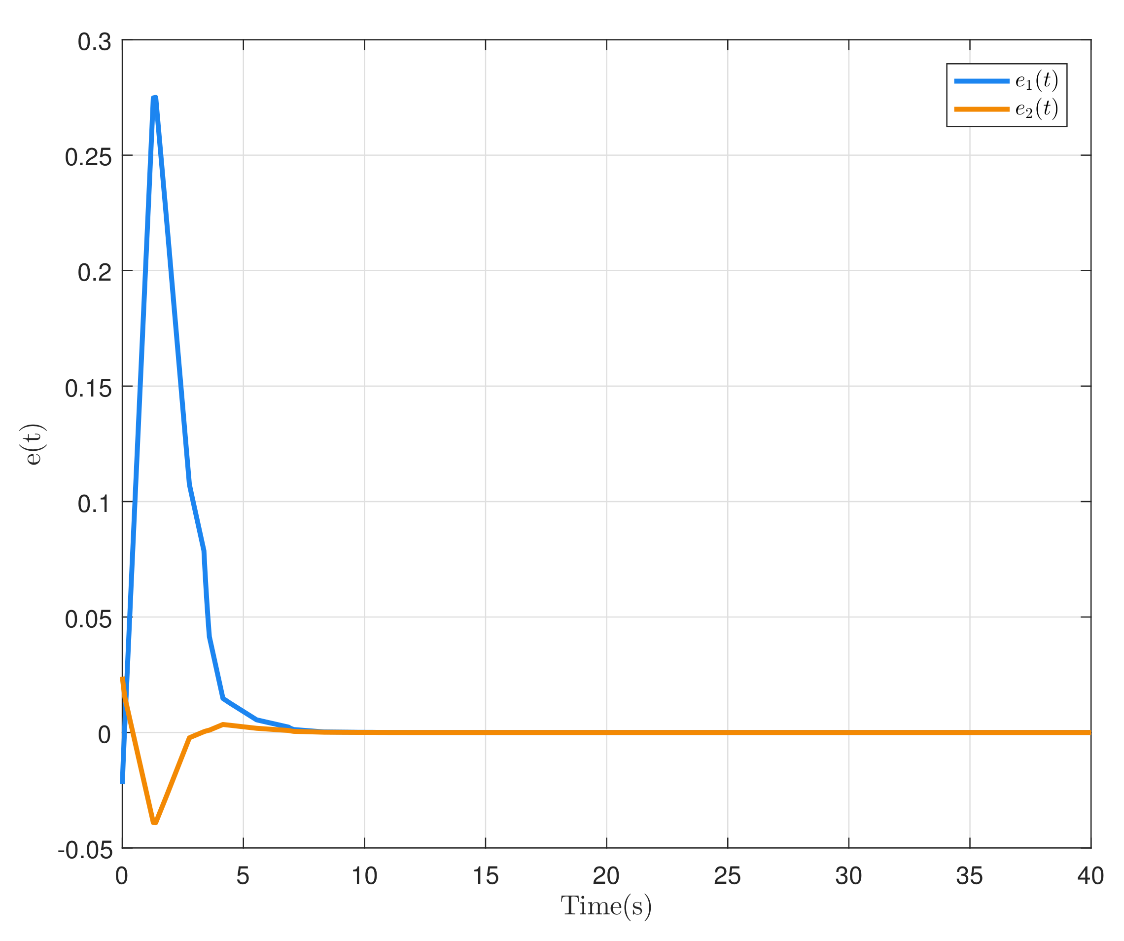
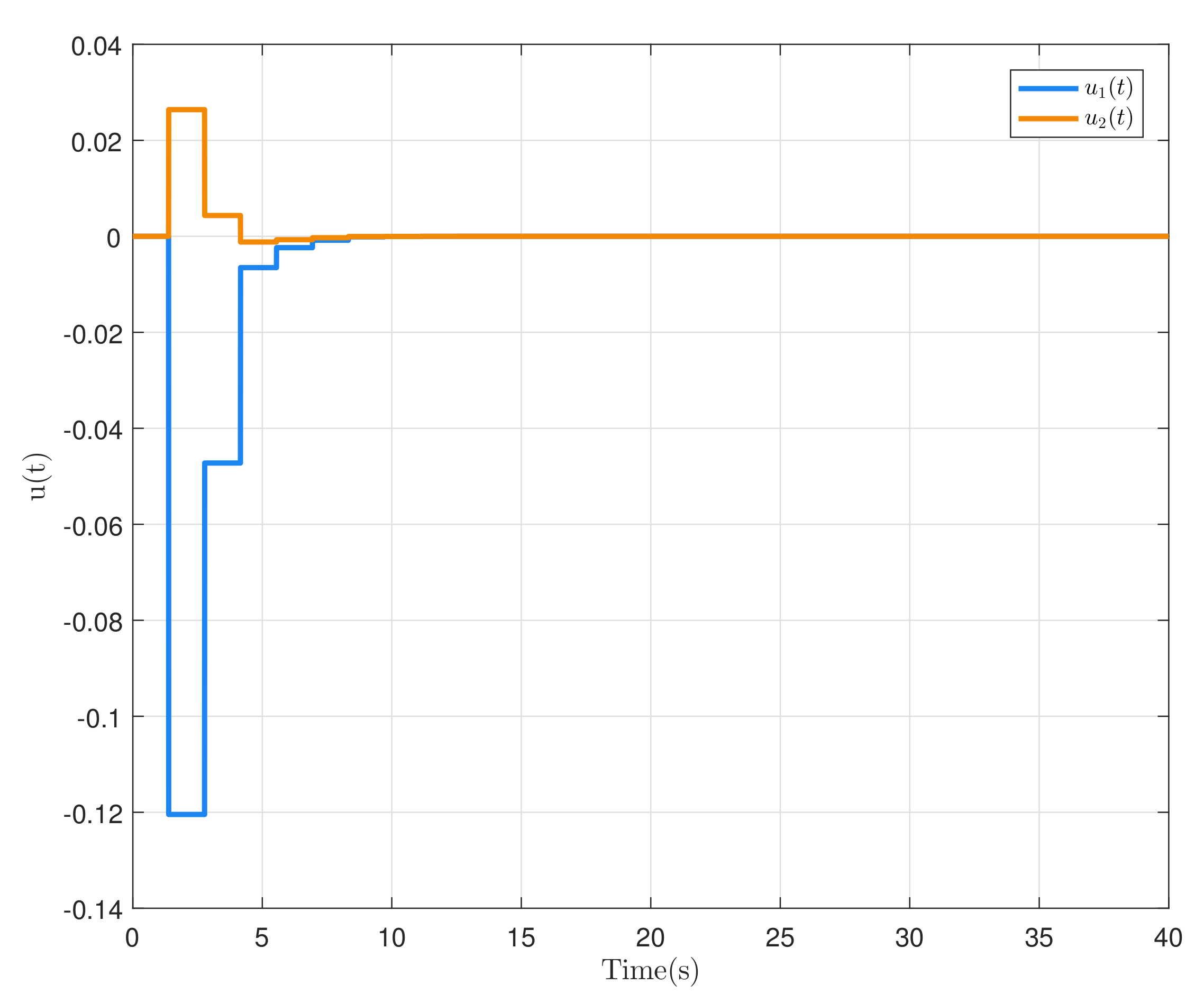
Furthermore, if we choose the neural activation functions as f i ( x i ) = t a n h ( x i ) ( i = 1 , 2 ) , τ 1 ( t ) = 0.5 s i n 2 ( 0.9 t ) , and τ 2 ( t ) = 2 c o s 2 ( 0.5 t ) , the initial condition e ( 0 ) = col { 1 , 1 } . The response curves of the error system (6) with u ( t ) are given in Figure 3, and the control input u ( t ) is shown in Figure 4. Figure 3 shows that the NTNNs with parameter uncertainties are stable at their equilibrium points, which verifies that the slave system (5) is synchronous with the master system (1).
Example 3. 
Consider the neutral-type neural networks (10) with the following parameters [17]:
A = 1 0 0 0.5 , W 0 = 1.8 0.15 5.2 1.5 , W 1 = 1.7 0.12 0.26 2.5 , W 2 = 0 0 0 0 .
The neural activation functions are taken as the form f i ( x i ) = t a n h ( x i ) ( i = 1 , 2 ) , which satisfies the assumption (7) with K = diag ( 0 , 0 ) , K + = diag ( 1 , 1 ) . The time-delay τ ( t ) = e t / ( e t + 1 ) . The initial condition of the master system and the slave system is taken as x ( 0 ) = col ( 0.2 , 0.3 ) , y ( 0 ) = col ( 0.3 , 0.6 ) and u ( t ) = 0 . For given scalars τ 2 = 1 , μ 2 = 0.25 , via solving the LMIs in Corollary 3, the derived maximum sampling intervals of the NTNNs for different communication delays τ c are obtained when ϵ 1 = ϵ 2 = 0.24 , and d k = d M . The results are shown in Table 3.
For various τ c , the maximum sampling period d M by Corollary 3 in this paper and the related methods in [26,27] are listed in Table 3. It can be found that Corollary 3 provides a larger maximum sampling period compared with the results of the literature in Table 3. It shows that the proposed criteria are less conservative than the ones in the literature. That is to say, the LKF containing a mixed delay part can lead to a less conservative result.
Based on Corollary 3, when τ c = 0.01 , the maximum sampling period d M = 0.2621 , the desired controller gain matrix can be calculated as
K = 4.2096 0.0865 0.8097 4.5161 .
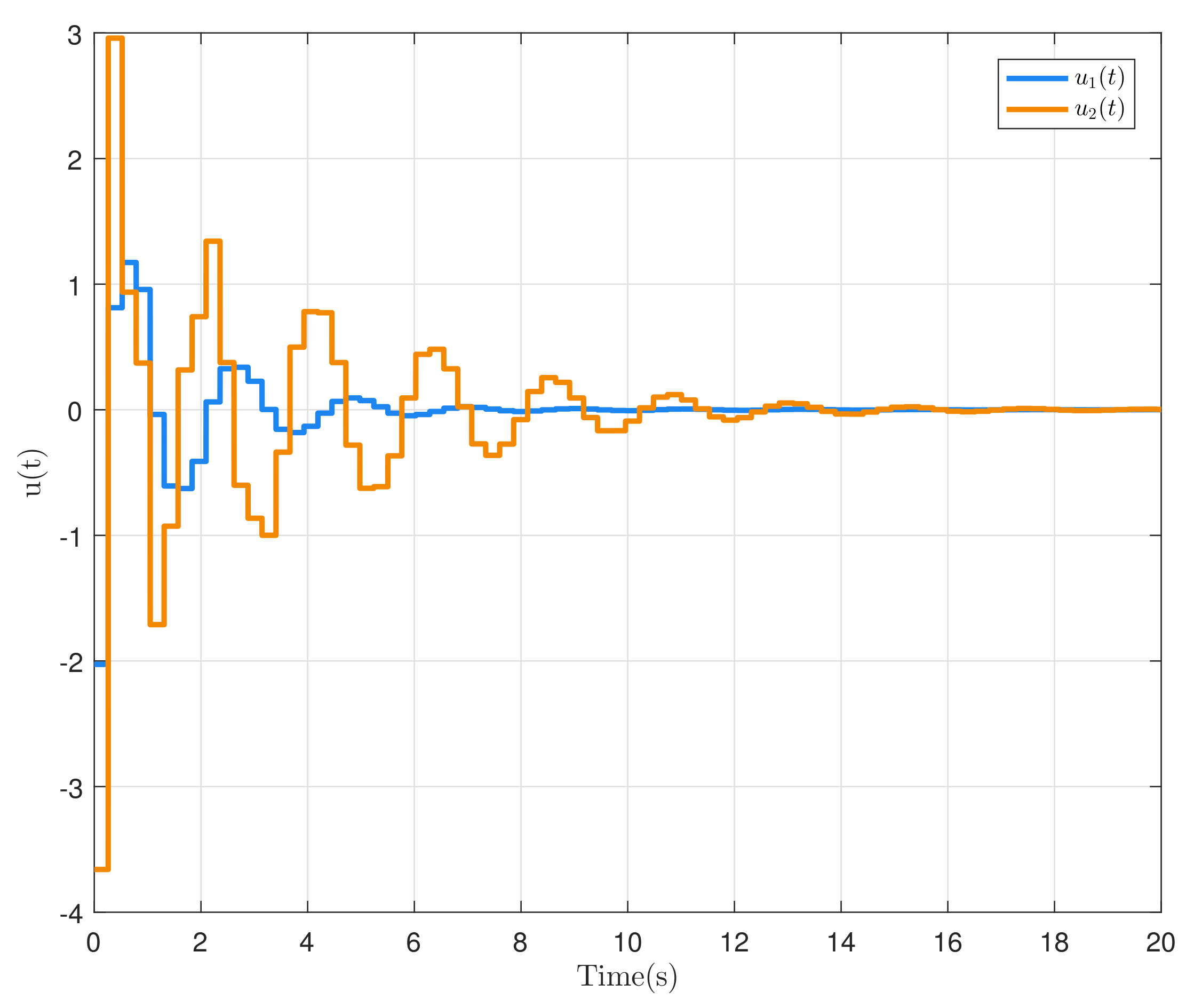
Based on the above sample-data controller, the state response curves of the error system (6) and the control input (9) are shown in Figure 5 and Figure 6, respectively. Figure 5 shows that the NNs are stable at their equilibrium points, which verifies that the error system is asymptotic stable. The slave system (5) is synchronous with the master system (1).

5. Discussion

A function that considers the information of the intervals [ t k , t ] , [ t k τ , t τ ] , [ t , t k + 1 ) and [ t τ , t k + 1 τ ) is known as a two-sided looped functional. As more state information is taken into account, a less conservative stability criterion will be developed. The sample-data control approach can increase the control effectiveness while reducing network congestion. However, in practical implementations, communication delays are unavoidable when signals are sent from the sampler to the controller. Our limited knowledge indicates that there is no research that investigate NTNNs synchronization control using a sample-data controller considering communication delay. These factors prompt our investigation on NTNNs synchronization control.
In addition, systems with a single delay were the main subject of the research. Any form of time delay might be detrimental to the practical synchronization control of NTNNs. An important area for research is how the interaction between the delays affect each other. The connection between transmission delay and communication delay as well as the interconnectedness between neutral delay and transmission delay are all taken into account in this work. Three examples show that a mixed-delay-dependent LKF may lead to a less conservative criterion. Therefore, future research will concentrate on gathering more information of the delays and exploring ways to relax the restrictions placed on LKF.
In this article, the integral terms of the derivative of the LKF are estimated by using a free-matrix-based integral inequality. This approach produces a large number of free matrices, which makes the calculations more complex. Therefore, future study will concentrate on finding ways to improve the result by decreasing the LKF limitations and achieving a less conservative criterion.

6. Conclusions

In this study, we present a sampled-data synchronization scheme for uncertain NTNNs. A new LKF with a mixed-delay-dependent augmented part and a two-sided looped part is proposed. Benefiting from the LKF, two synchronization criteria are derived to guarantee the stability of the error systems, thereby allowing the slave system to synchronize with the master systems. Based on the criterion, a corresponding sampled-data controller scheme with a communication delay is designed. Finally, the validity of the proposed criteria is demonstrated through three numerical examples.

Author Contributions

Conceptualization, S.W. and K.S.; formal analysis, S.W. and K.S.; funding acquisition, K.S.; methodology, S.W. and K.S.; project administration, K.S.; software, S.W.; supervision, K.S.; validation, S.W.; visualization, S.W.; writing—original draft, S.W.; writing—review and editing, K.S. All authors have read and agreed to the published version of the manuscript.

Funding

This work was supported by the Opening Fund of Geomathematics Key Laboratory of Sichuan Province (scsxdz2018zd04 and scsxdz2020zd01) and Sichuan Science and Technology Program under Grant Nos. 21YYJC0469 and 23ZDYF0645.

Institutional Review Board Statement

Not applicable.

Informed Consent Statement

Not applicable.

Data Availability Statement

Not applicable.

Conflicts of Interest

The authors declare no conflict of interest.

Appendix A

Proof. 
We choose the following LKFs candidates as
V ( t ) = i = 1 5 V i ( t ) + j = 1 4 W j ( t ) ,
where
V 1 ( t ) = ϖ 1 T ( t ) P 1 ϖ 1 ( t ) + 2 i = 1 n λ 1 i 0 e i ( t ) f i ( s ) k i s d s + 2 i = 1 n λ 2 i 0 e i ( t ) k i + s f i ( s ) d s , V 2 ( t ) = t τ 2 ( t ) t ϖ 2 T ( s ) P 2 ϖ 2 ( s ) d s + t τ 1 ( t ) t e ˙ T ( s ) P 3 e ˙ ( s ) d s , V 3 ( t ) = t τ 1 t ϖ 3 T ( s ) X 1 ϖ 3 ( s ) d s + t τ 2 t ϖ 3 T ( s ) X 2 ϖ 3 ( s ) + t τ c t ϖ 3 T ( s ) X 3 ϖ 3 ( s ) d s , V 4 ( t ) = t τ 2 t τ 1 e T ( s ) X 4 e ( s ) d s + τ 2 τ 1 t + θ t e ˙ T ( u ) X 5 e ˙ ( u ) d u d θ + t τ c t τ 2 e T ( s ) X 6 e ( s ) d s , V 5 ( t ) = τ 1 0 t + θ t e ˙ T ( u ) S 1 e ˙ ( u ) d u d θ + τ 2 0 t + θ t e ˙ T ( u ) S 2 e ˙ ( u ) d u d θ + τ c 0 t + θ t e ˙ T ( u ) Z 1 e ˙ ( u ) d u d θ + η M τ c t + θ t e ˙ T ( u ) Z 2 e ˙ ( u ) d u d θ + η M 0 t + θ t e ˙ T ( u ) Z 3 e ˙ ( u ) d u d θ ,
W 1 ( t ) = 2 ϖ 4 T ( t ) ( Q 1 ϖ 5 ( t ) + Q 2 ϖ 6 ( t ) ) , W 2 ( t ) = ( t k + 1 t ) ( t t k ) ϖ 6 T ( t ) Q 3 ϖ 6 ( t ) , W 3 ( t ) = ( t k + 1 t ) ( t t k ) ϖ 7 ( t ) T Q 4 ϖ 7 ( t ) , W 4 ( t ) = ( t k + 1 t ) t k t e ˙ T ( s ) R 1 e ˙ ( s ) d s ( t t k ) t t k + 1 e ˙ T ( s ) R 2 e ˙ ( s ) d s + ( t k + 1 t ) t k τ c t τ c e ˙ T ( s ) R 3 e ˙ ( s ) d s ( t t k ) t τ c t k + 1 τ c e ˙ T ( s ) R 4 e ˙ ( s ) d s
Taking the derivatives of V ( t ) along the trajectory of the error system (6) yields
V ˙ 1 ( t ) = ξ T ( t ) Sym Ω 1 T P 1 Ω 2 + ( r 11 K p r 1 ) T Δ 1 r 8 + ( K m r 1 r 11 ) T Δ 2 r 8 ξ ( t ) , V ˙ 2 ( t ) ξ T ( t ) Ω 3 T P 2 Ω 3 ( 1 u 2 ) Ω 4 T P 2 Ω 4 + r 8 T P 3 r 8 ( 1 u 1 ) r 26 T P 3 r 26 ξ ( t ) , V ˙ 3 ( t ) ξ T ( t ) Ω 5 T ( X 1 + X 2 + X 3 ) Ω 5 Ω 6 T X 1 Ω 6 Ω 7 T X 2 Ω 7 Ω 8 T X 3 Ω 8 ξ ( t ) , V ˙ 4 ( t ) = ξ T ( t ) r 24 T X 4 r 24 r 11 T X 4 r 11 + τ 21 r 8 T X 5 r 8 + r 11 T X 6 r 11 r 2 T X 6 r 2 ξ ( t ) + J 0 , V ˙ 5 ( t ) = ξ T ( t ) τ 1 r 8 T S 1 r 8 + τ 2 r 8 T S 2 r 8 + τ c r 8 T Z 1 r 8 + d M r 8 T Z 2 r 8 + η M r 8 T Z 3 r 8 ξ ( t ) + J 1 + J 2 + J 3 + J 4 + J 5 , W ˙ 1 ( t ) = ξ T ( t ) Sym Ω 9 T ( Q 1 Ω 10 + Q 2 Ω 11 ) + ( t k + 1 t ) ( Ω 12 T ( Q 1 Ω 10 + Q 2 Ω 11 ) + Ω 13 T Q 1 Ω 14 ) + ( t t k ) ( Ω 15 T ( Q 1 Ω 10 + Q 2 Ω 11 ) + Ω 16 T Q 1 Ω 14 ) ξ ( t ) , W ˙ 2 ( t ) = ξ T ( t ) ( ( t k + 1 t ) ( t t k ) ) Ω 11 T Q 3 Ω 11 ξ ( t ) , W ˙ 3 ( t ) = ξ T ( t ) ( t k + 1 t ) Sym Ω 17 T Q 4 Ω 18 + Ω 17 T Q 4 Ω 17 + ( t t k ) Sym Ω 17 T Q 4 Ω 19 Ω 17 T Q 4 Ω 17 ξ ( t ) , W ˙ 4 ( t ) = ξ T ( t ) ( t k + 1 t ) ( r 8 T R 1 r 8 + r 9 T R 3 r 9 ) + ( t t k ) ( r 8 T R 2 r 8 + r 9 T R 4 r 9 ) ξ ( t ) + J 6 + J 7 + J 8 + J 9 ,
where
J 0 = t τ 2 t τ 1 e ˙ T ( s ) X 5 e ˙ ( s ) d s , J 1 = t τ 1 t e ˙ T ( s ) S 1 e ˙ ( s ) d s , J 2 = t τ 2 t e ˙ T ( s ) S 2 e ˙ ( s ) d s , J 3 = t τ c t e ˙ T ( s ) Z 1 e ˙ ( s ) d s , J 4 = t η M t τ c e ˙ T ( s ) Z 2 e ˙ ( s ) d s , J 5 = t η M t e ˙ T ( s ) Z 3 e ˙ ( s ) d s , J 6 = t k t e ˙ T ( s ) R 1 e ˙ ( s ) d s , J 7 = t t k + 1 e ˙ T ( s ) R 2 e ˙ ( s ) d s , J 8 = t k τ c t τ c e ˙ T ( s ) R 3 e ˙ ( s ) d s , J 9 = t τ c t k + 1 τ c e ˙ T ( s ) R 4 e ˙ ( s ) d s .
From η M η k and Z 2 + Z 3 > 0 , the integral quadratic terms can be rearranged as
i = 0 9 J i t τ 1 t e ˙ T ( s ) S 1 e ˙ ( s ) d s t τ 2 t e ˙ T ( s ) S 2 e ˙ ( s ) d s t τ c t e ˙ T ( s ) Z 1 e ˙ ( s ) d s t t k + 1 e ˙ T ( s ) R 2 e ˙ ( s ) d s t k t e ˙ T ( s ) ( R 1 + Z 3 ) e ˙ ( s ) d s t k τ c t τ c e ˙ T ( s ) ( R 3 + Z 2 ) e ˙ ( s ) d s t τ c t k + 1 τ c e ˙ T ( s ) R 4 e ˙ ( s ) d s t k τ c t k e ˙ T ( s ) Z 3 e ˙ ( s ) d s t η k t k τ c e ˙ T ( s ) ( Z 2 + Z 3 ) e ˙ ( s ) d s t τ 2 t τ 1 e ˙ T ( s ) X 5 e ˙ ( s ) d s .
Using Lemma 1 to estimate J i ( i = 0 , 1 , , 9 ) , we obtain
i = 0 9 J i ξ T ( t ) Π T { τ c i = 1 3 1 2 i 1 Y i Z 1 1 Y i T Π + τ c Y 14 Z 3 1 Y 14 T Π + τ 2 i = 1 2 1 2 i 1 Y 15 + i S 2 1 Y 15 + i T Π + τ 1 Y 18 S 1 1 Y 18 T Π + τ 21 Y 19 X 5 1 Y 19 T Π + ( t t k ) [ i = 1 3 1 2 i 1 Y 6 + i ( R 1 + Z 3 ) 1 Y 6 + i T Π + i = 1 2 1 2 i 1 Y 9 + i ( R 3 + Z 2 ) 1 Y 9 + i T Π ] + ( t k + 1 t ) [ i = 1 3 1 2 i 1 Y 3 + i R 2 1 Y 3 + i T Π + i = 1 2 1 2 i 1 Y 11 + i R 4 1 Y 11 + i T Π + Y 15 ( Z 2 + Z 3 ) 1 Y 15 T Π ] + Sym i = 1 19 Y i i ξ ( t ) .
For given scalars ϵ 1 , ϵ 2 and any matrix G with appropriate dimensions, the following equations hold:
0 = 2 e T ( t ) + ϵ 1 e T ( t k τ c ) + ϵ 2 e ˙ T ( t ) G e ˙ ( t ) A e ( t ) + W 0 f ( e ( t ) ) + W 1 f ( e ( t τ 2 ( t ) ) ) + W 2 e ˙ ( t τ 1 ( t ) ) + K e ( t k τ c ) = 2 ξ T ( t ) Ω 20 T Ω 21 ξ ( t ) ,
where L = G K , and the controller gain matrix in (6) can be calculated by
K = G 1 L .
To make use of the information of the activation function (7), we can obtain
0 i = 1 n δ 1 i f i ( e i ( t ) ) k i e i ( t ) k i + e i ( t ) f i ( e i ( t ) ) = 2 ξ T ( t ) Ω 22 T U Ω 23 ξ ( t ) , 0 i = 1 n δ 2 i f i ( e i ( t τ 2 ( t ) ) ) k i e i ( t τ 2 ( t ) ) k i + e i ( t τ 2 ( t ) ) f i ( e i ( t τ 2 ( t ) ) )
= 2 ξ T ( t ) Ω 24 T V Ω 25 ξ ( t ) ,
where U = diag δ 11 , δ 12 , , δ 1 n 0 , V = diag δ 21 , δ 22 , , δ 2 n 0 .
Adding the right-hand sides of (A2)–(A5) into V ˙ ( t ) , we can obtain
V ˙ ( t ) ξ T ( t ) t k + 1 t d k Ξ 1 + t t k d k Ξ 2 ξ ( t ) ,
where Ξ 1 = Γ 1 + d k Γ 2 + Γ 4 , Ξ 2 = Γ 1 + d k Γ 3 + Γ 5 , and Γ j ( j = 1 , 2 , 3 , 4 , 5 ) are defined in Theorem 1.
Note that the LMIs (14) and (15) are equal to Ξ 1 < 0 and Ξ 2 < 0 based on the Schur complement, respectively. That is to say, if the inequality conditions of the LMIs (14) and (15) hold, it can guarantee V ˙ ( t ) σ e ( t ) 2 for a sufficient small scalar σ > 0 . Then, the synchronization error system (6) is asymptotically stable, and the slave system is synchronized with the master system. This completes the proof. □

Appendix B

Proof. 
We choose the following LKFs candidates as
V ( t ) = V ^ 1 ( t ) + V 2 ( t ) + V 3 ( t ) + V 5 ( t ) + j = 1 4 W j ( t ) ,
where
V ^ 1 ( t ) = e T ( t ) P 1 e ( t ) + 2 i = 1 n λ 1 i 0 e i ( t ) f i ( s ) k i s d s + 2 i = 1 n λ 2 i 0 e i ( t ) k i + s f i ( s ) d s ,
as a result,
V ˙ 1 ( t ) = ξ T ( t ) Sym r 1 T P 1 r 8 + ( r 11 K r 1 ) T Δ 1 r 8 + ( K + r 1 r 11 ) T Δ 2 r 8 ξ ( t ) .
The rest of the process is similar to that in the proof of Theorem 1, and hence, we omit it here. □

Appendix C

Proof. 
Based on the LMI results in Theorem 1, replacing A , W 0 , W 1 and W 2 with A + F Σ ( t ) E 1 , W 0 + F Σ ( t ) E 2 , W 1 + F Σ ( t ) E 3 and W 2 + F Σ ( t ) E 4 , respectively, we can check that the derived inequalities are equivalent to the following terms:
Ξ ^ 1 = Ξ 1 + Ψ 1 Σ ( t ) Ψ 2 T + ( Ψ 1 Σ ( t ) Ψ 2 T ) T < 0 ,
Ξ ^ 2 = Ξ 2 + Ψ 1 Σ ( t ) Ψ 2 T + ( Ψ 1 Σ ( t ) Ψ 2 T ) T < 0 .
Now by utilizing Lemma 2, there exist two positive scalars σ i > 0 ( i = 1 , 2 ) , such that
Ξ ^ 1 = Ξ 1 + σ 1 1 Ψ 1 T σ 1 Ψ 2 T T I J J T I 1 σ 1 1 Ψ 1 T σ 1 Ψ 2 T < 0 ,
Ξ ^ 2 = Ξ 2 + σ 2 1 Ψ 1 T σ 2 Ψ 2 T T I J J T I 1 σ 2 1 Ψ 1 T σ 2 Ψ 2 T < 0 .
Then by setting δ n = σ i 2 ( n = 1 , 2 ) , it is easy to verify that Ξ ^ 1 < 0 and Ξ ^ 2 < 0 are equal to the LMIs (20) and (21) based on the Schur complement. The rest of the process is similar to that in the proof of Theorem 1; hence, we omit it here. □

Appendix D

Proof. 
We choose the following LKFs candidates as
V ( t ) = V ^ 1 ( t ) + V 2 ( t ) + V 3 ( t ) + V 5 ( t ) + j = 1 4 W j ( t ) ,
where
V ^ 1 ( t ) = e T ( t ) P 1 e ( t ) + 2 i = 1 n λ 1 i 0 e i ( t ) f i ( s ) k i s d s + 2 i = 1 n λ 2 i 0 e i ( t ) k i + s f i ( s ) d s ,
as a result,
V ˙ 1 ( t ) = ξ T ( t ) Sym r 1 T P 1 r 8 + ( r 11 K r 1 ) T Δ 1 r 8 + ( K + r 1 r 11 ) T Δ 2 r 8 ξ ( t ) .
The rest of the process is similar to that in the proof of Theorem 1; hence, we omit it here. □

Appendix E

Proof. 
We choose the following LKFs candidates as
V ( t ) = i = 1 5 V ˜ i ( t ) + j = 1 4 W j ( t ) ,
where
V ˜ 1 ( t ) = ϖ ˜ 1 T ( t ) P 1 ϖ ˜ 1 ( t ) + 2 i = 1 n λ 1 i 0 e i ( t ) f i ( s ) k i s d s + 2 i = 1 n λ 2 i 0 e i ( t ) k i + s f i ( s ) d s , V ˜ 2 ( t ) = t τ 2 ( t ) t ϖ 2 T ( s ) P 2 ϖ 2 ( s ) d s , V ˜ 3 ( t ) = t τ 2 t ϖ 3 T ( s ) X 2 ϖ 3 ( s ) + t τ c t ϖ 3 T ( s ) X 3 ϖ 3 ( s ) d s , V ˜ 4 ( t ) = t τ c t τ 2 e T ( s ) X 6 e ( s ) d s , V ˜ 5 ( t ) = τ 2 0 t + θ t e ˙ T ( u ) S 1 e ˙ ( u ) d u d θ + τ c 0 t + θ t e ˙ T ( u ) Z 1 e ˙ ( u ) d u d θ + η M τ c t + θ t e ˙ T ( u ) Z 2 e ˙ ( u ) d u d θ + η M 0 t + θ t e ˙ T ( u ) Z 3 e ˙ ( u ) d u d θ . ϖ ˜ 1 ( t ) = col e ( t ) , e ( t τ c ) , e ( t τ 2 ) , τ c v 5 ( t ) τ 2 v 13 ( t ) , τ c 2 v 6 ( t ) , ξ ˜ ( t ) = col e ( t ) , e ( t τ c ) , e ( t k ) , e ( t k τ c ) , e ( t k + 1 ) , e ( t k + 1 τ c ) , e ( t η k ) , e ˙ ( t ) , e ˙ ( t τ c ) , e ˙ ( t τ 2 ) , e ( t τ 2 ) , e ( t τ 2 ( t ) ) , f ( e ( t ) ) , f ( e ( t τ 2 ( t ) ) ) , v 5 ( t ) , v 6 ( t ) , v 7 ( t ) , v 8 ( t ) , v 9 ( t ) , v 10 ( t ) , v 11 ( t ) , v 12 ( t ) , v 13 ( t ) .
The rest of the proof process is similar to that in the proof of Theorem 2; hence, we omit it here. □

References

  1. Egmont-Petersen, M.; de Ridder, D.; Handels, H. Image processing with neural networks—A review. Pattern Recognit. 2002, 35, 2279–2301. [Google Scholar] [CrossRef]
  2. Kothari, S.; Oh, H. Neural Networks for Pattern Recognition. Adv. Comput. 1993, 37, 119–166. [Google Scholar]
  3. Mestari, M.; Benzirar, M.; Saber, N.; Khouil, M. Solving Nonlinear Equality Constrained Multiobjective Optimization Problems Using Neural Networks. IEEE Trans. Neural Netw. Learn Syst. 2015, 26, 2500–2520. [Google Scholar] [CrossRef]
  4. Chen, Y.H.; Fang, S.C. Neurocomputing with time delay analysis for solving convex quadratic programming problems. IEEE Trans. Neural Netw. Learn Syst. 2000, 11, 230–240. [Google Scholar] [CrossRef]
  5. Zhang, J. Globally exponential stability of neural networks with variable delays. IEEE Trans. Circuits Syst. I Fundam. Theory Appl. 2003, 50, 288–290. [Google Scholar] [CrossRef]
  6. Lv, Y.; Lv, W.; Sun, J. Convergence dynamics of stochastic reaction-diffusion recurrent neural networks with continuously distributed delays. Nonlinear Anal. Real World Appl. 2008, 9, 1590–1606. [Google Scholar] [CrossRef]
  7. Shi, K.; Zhu, H.; Zhong, S.; Zeng, Y.; Zhang, Y. New stability analysis for neutral type neural networks with discrete and distributed delays using a multiple integral approach. J. Frankl. Inst. 2015, 352, 155–176. [Google Scholar] [CrossRef]
  8. Kolmanovskii, V.B.; Nosov, V.R. Stability of Functional Differential Equations; Academic: London, UK, 1986. [Google Scholar]
  9. Kuang, Y. Delay Differential Equations with Applications in Population Dynamics; Academic: Boston, MA, USA, 1993. [Google Scholar]
  10. Cai, X.; Shi, K.; She, K.; Zhong, S.; Tang, Y. Quantized Sampled-Data Control Tactic for T-S Fuzzy NCS Under Stochastic Cyber-Attacks and Its Application to Truck-Trailer System. IEEE Trans. Veh. Technol. 2022, 71, 7023–7032. [Google Scholar] [CrossRef]
  11. Cai, X.; Shi, K.; She, K.; Zhong, S.; Soh, Y.; Yu, Y. Performance Error Estimation and Elastic Integral Event Triggering Mechanism Design for T-S Fuzzy Networked Control System Under DoS Attacks. IEEE Trans. Fuzzy Syst. 2022, 1–12. [Google Scholar] [CrossRef]
  12. Fridman, E.; Seuret, A.; Richard, J.P. Robust sampled-data stabilization of linear systems: An input delay approach. Automatica 2004, 40, 1441–1446. [Google Scholar] [CrossRef]
  13. Fujioka, H. A Discrete-Time Approach to Stability Analysis of Systems With Aperiodic Sample-and-Hold Devices. IEEE Trans. Autom. Control 2009, 54, 2440–2445. [Google Scholar] [CrossRef] [Green Version]
  14. Naghshtabrizi, P.; Hespanha, J.P.; Teel, A.R. Exponential stability of impulsive systems with application to uncertain sampled-data systems. Syst. Control Lett. 2008, 57, 378–385. [Google Scholar] [CrossRef]
  15. Zeng, H.B.; Teo, K.; He, Y. A new looped-functional for stability analysis of sampled-data systems. Automatica 2017, 82, 328–331. [Google Scholar] [CrossRef]
  16. Zeng, H.B.; Zhai, Z.L.; He, Y.; Teo, K.L.; Wang, W. New insights on stability of sampled-data systems with time-delay. Appl. Math. Comput. 2020, 374, 125041. [Google Scholar] [CrossRef]
  17. Zeng, H.B.; Zhai, Z.L.; Yan, H.; Wang, W. A New Looped Functional to Synchronize Neural Networks With Sampled-Data Control. IEEE Trans. Neural Netw. Learn Syst. 2022, 33, 406–415. [Google Scholar] [CrossRef]
  18. Zhang, Y.; He, Y.; Long, F.; Zhang, C.K. Mixed-Delay-Based Augmented Functional for Sampled-Data Synchronization of Delayed Neural Networks With Communication Delay. IEEE Trans. Neural Netw. Learn Syst. 2022, 1–10. [Google Scholar] [CrossRef] [PubMed]
  19. Zhang, G.; Wang, T.; Li, T.; Fei, S. Multiple integral Lyapunov approach to mixed-delay-dependent stability of neutral neural networks. Neurocomputing 2018, 275, 1782–1792. [Google Scholar] [CrossRef]
  20. Zhang, H.; Ma, Q.; Lu, J.; Chu, Y.; Li, Y. Synchronization control of neutral-type neural networks with sampled-data via adaptive event-triggered communication scheme. J. Frankl. Inst. 2021, 358, 1999–2014. [Google Scholar] [CrossRef]
  21. Zeng, H.B.; He, Y.; Wu, M.; She, J. New results on stability analysis for systems with discrete distributed delay. Automatica 2015, 60, 189–192. [Google Scholar] [CrossRef]
  22. Li, T.; Guo Song, A.; Min Fei, S. Robust stability of stochastic Cohen–Grossberg neural networks with mixed time-varying delays. Neurocomputing 2009, 73, 542–551. [Google Scholar] [CrossRef]
  23. Seuret, A. A novel stability analysis of linear systems under asynchronous samplings. Automatica 2012, 48, 177–182. [Google Scholar] [CrossRef] [Green Version]
  24. Liu, P.L. Further improvement on delay-dependent robust stability criteria for neutral-type recurrent neural networks with time-varying delays. ISA Trans. 2015, 55, 92–99. [Google Scholar] [CrossRef]
  25. Yin, C.; Cheng, Y.; Huang, X.; ming Zhong, S.; Li, Y.; Shi, K. Delay-partitioning approach design for stochastic stability analysis of uncertain neutral-type neural networks with Markovian jumping parameters. Neurocomputing 2016, 207, 437–449. [Google Scholar] [CrossRef]
  26. Wei, W.; Zeng, H.B.; Teo, K.L. Free-matrix-based time-dependent discontinuous Lyapunov functional for synchronization of delayed neural networks with sampled-data control. Chin. Phys. B 2017, 26, 127–134. [Google Scholar]
  27. Xiao, S.P.; Lian, H.H.; Teo, K.L.; Zeng, H.B.; Zhang, X.H. A new Lyapunov functional approach to sampled-data synchronization control for delayed neural networks. J. Frankl. Inst. 2018, 355, 8857–8873. [Google Scholar] [CrossRef]
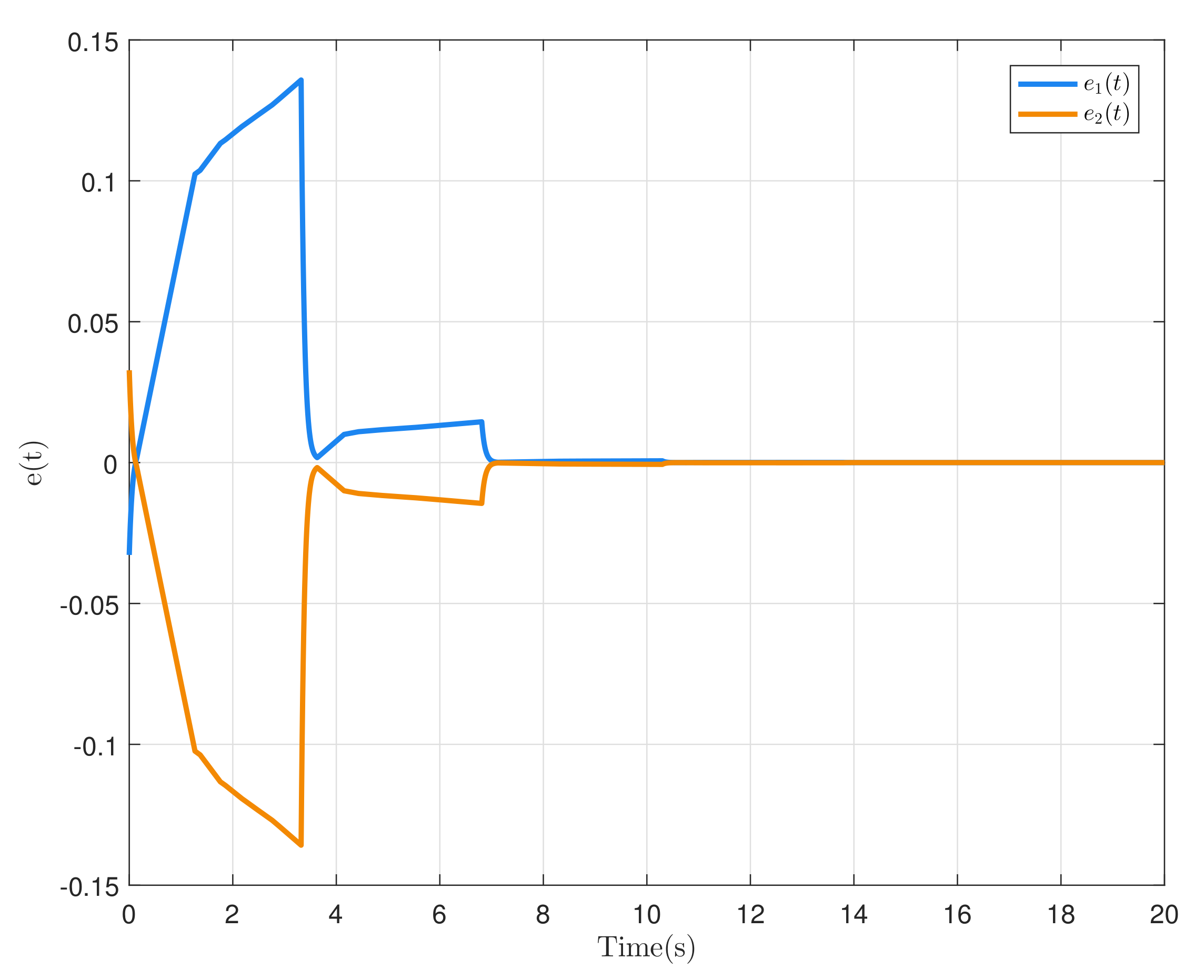
Figure 1. State responses of the error system.
Mathematics 11 00872 g001
Figure 2. Control input u ( t ) .
Mathematics 11 00872 g002
Figure 3. State responses of the error system.
Mathematics 11 00872 g003
Figure 4. Control input u ( t ) .
Mathematics 11 00872 g004
Figure 5. State responses of the error system.
Mathematics 11 00872 g005
Figure 6. Control input u ( t ) .
Mathematics 11 00872 g006
Table 1. The maximum sampling period d M for different τ c (Example 1).
τ c 0.010.030.050.070.09
Corollary 11.37661.34991.32961.31341.2996
Theorem 11.38811.38651.38201.37771.3738
Improvement0.835%4.9406%3.9411%4.8957%5.7094%
Table 2. The maximum sampling period d M with parameter uncertainties (Example 2).
τ c 0.010.030.050.070.09
Corollary 225.963124.168222.609721.243720.0398
Theorem 226.213425.268624.397023.474122.5952
Improvement0.964%4.5530%7.9050%10.4991%12.7516%
Table 3. The maximum sampling period d M for different τ c (Example 2).
τ c 0.010.030.050.070.09
[26]      0.23      0.19      0.16      0.13      0.10
[27]      0.24      0.20      0.17      0.13      0.10
Corollary 3      0.26      0.21      0.17      0.14      0.10
Disclaimer/Publisher’s Note: The statements, opinions and data contained in all publications are solely those of the individual author(s) and contributor(s) and not of MDPI and/or the editor(s). MDPI and/or the editor(s) disclaim responsibility for any injury to people or property resulting from any ideas, methods, instructions or products referred to in the content.