A Structure-Preserving Finite Volume Scheme for a Hyperbolic Reformulation of the Navier–Stokes–Korteweg Equations

Abstract

In this paper, we present a new explicit second-order accurate structure-preserving finite volume scheme for the first-order hyperbolic reformulation of the Navier–Stokes–Korteweg equations. The model combines the unified Godunov-Peshkov-Romenski model of continuum mechanics with a recently proposed hyperbolic reformulation of the Euler–Korteweg system. The considered PDE system includes an evolution equation for a gradient field that is by construction endowed with a curl-free constraint. The new numerical scheme presented here relies on the use of vertex-based staggered grids and is proven to preserve the curl constraint exactly at the discrete level, up to machine precision. Besides a theoretical proof, we also show evidence of this property via a set of numerical tests, including a stationary droplet, non-condensing bubbles as well as non-stationary Ostwald ripening test cases with several bubbles. We present quantitative and qualitative comparisons of the numerical solution, both, when the new structure-preserving discretization is applied and when it is not. In particular for under-resolved simulations on coarse grids we show that some numerical solutions tend to blow up when the curl-free constraint is not respected.

1. Introduction

Many models of mechanics and physics in general are described by a set of evolution equations, in which some state variables are also subject to stationary differential constraints (involutions), restricting the set of admissible solutions. Some of the most notable examples are constraints on the divergence or the curl of a given field, which are encountered for example when dealing with Maxwell’s equations of electrodynamics or with magneto-hydrodynamics, which require the magnetic field to be divergence-free for all times. In many cases, the constraints are supplied as an extra equation to the system, i.e., a given field obeys a time-evolution equation, but is also bound independently by an additional property. This is the case, for example, in the incompressible Navier–Stokes equations. The time evolution of the velocity field is governed by the momentum conservation equation, but has to also satisfy a supplementary divergence-free constraint due to the incompressibility assumption. We call the constraint supplementary because it is not a consequence of the evolution equations, but an additional property. In the incompressible Navier–Stokes equations the divergence-free condition is actually the pressure equation, see, e.g., [1,2,3]: even if the velocity is divergence-free initially, there is no guarantee that it remains so for later times by means of its evolution equation alone.

Yet, in some other examples, it occurs that the constraint is intrinsic to the mathematical structure of the evolution equation, that is exact solutions verify it by nature. For instance, a potential flow has an intrinsic curl-free constraint on the velocity, since the latter is expressed as the gradient of a scalar field. Thus, at the theoretical level, the solutions verify the curl-free constraint by nature. In Maxwell’s equations of electromagnetism, if the magnetic field is initially divergence-free, its time evolution equation ensures it remains so for later times. In such cases, we are talking about involution constraints, meaning they are direct consequences of the structure of the system and they do not need to be supplied independently. Several systems of different scopes and applications fall into this category, like the general symmetric hyperbolic and thermodynamically compatible (SHTC) class of PDEs forwarded by Godunov and Romenski and studied in [4,5,6,7,8,9], the multi-phase flow model of Romenski et al. [10] or first-order reductions of the Einstein field equations like those studied in [11,12,13].

While it might seem somewhat comforting that involution constraints are automatically satisfied by exact solutions of the PDE, provided that compatible initial conditions are given, this is a completely different story at the numerical level. Particular attention has to be directed to such constraints, even if they are an intrinsic property of the system at the continuous level. Indeed, the accumulation of discretization errors over the course of a numerical simulation can lead to the violation of curl-free or divergence-free constraints. This leads to numerical solutions that are neither compatible with the physics of the studied system, nor with its mathematical structure, see for example [14,15,16]. In some cases, the buildup of such errors can lead to unstable numerical simulations and to finite-time blowups [17,18]. The aforementioned issues have stimulated a lot of research in numerical analysis for hyperbolic PDE in recent years in order to develop better techniques and specific numerical methods that are able to address these notorious problems and provide numerical results that are compatible with the mathematical structure of the equations and with the underlying physics. Such techniques include for instance the so-called constrained transport methods [19,20,21,22,23,24,25,26], the Generalized-Lagrangian multiplier divergence-cleaning approach of Munz et al. [27,28,29,30], which was later also extended to hyperbolic curl cleaning in [13,18,31,32], as well as mimetic discretizations and reconstructions [16,33,34,35,36,37].

Recently, a novel first-order hyperbolic reformulation of the Navier–Stokes–Korteweg (NSK) system was proposed in [32]. The NSK equations can be seen as a general model for viscous flows coupled with the Van der Waals second-gradient theory and serves as a model for compressible multiphase flows. Together with its dissipationless counterpart, that is the Euler–Korteweg system (EK), it was the subject of several works in recent decades, out of which we point out a few [38,39,40,41,42,43,44,45,46,47,48,49,50]. Alternative relaxation methods leading to parabolic approximations of different variants of the NSK system were also considered by Rohde and collaborators in [51,52,53,54,55,56]. For alternative hyperbolic diffuse interface models for compressible multiphase flows, the reader may refer to this non-exhaustive selection of references [57,58,59,60,61,62,63,64,65,66,67,68,69,70].

The hyperbolic reformulation of the NSK system incorporates a hyperbolic relaxation model of the EK Equations [71,72,73] into the unified Godunov-Peshkov-Romenski (GPR) model of continuum mechanics [4,5,6,7]. It admits a curl-involution constraint, which will be the main obstacle to address. The current paper is a natural sequel to the previous work of the authors [32], where a hyperbolic Generalized Lagrangian Multiplier (GLM) curl cleaning technique was employed [13,18,31]. In this paper, we design a new second-order accurate finite volume scheme, based on a carefully chosen vertex-based staggered grid, allowing to define a discrete gradient operator for which the discrete curl is identically null at the machine level. The scheme inherits most of its foundations from the works [17,74]. Similar techniques were developed previously for hyperbolic systems with divergence constraints, see for example [16,23,33,75,76,77]. Advantages of this type of method include for instance the fact that the PDE system in itself remains unchanged (unlike in GLM cleaning techniques for example) and that the discrete curl-errors are zero up to machine accuracy at the numerical level. This comes at the price of additional efforts in the implementation, as the method generally requires a well-chosen spatial discretization and a careful (staggered) positioning of the relevant variables.

The rest of this paper is organized as follows. In Section 2, we briefly recall the hyperbolic reformulation of the NSK model; we detail its structure and mathematical properties. In Section 3, we lay out the details of our new structure-preserving finite volume scheme. In particular, we describe the structure of the staggered computational grid, the splitting of the system, how each subsystem is evolved in time and how the compatible discrete differential operators are defined. Finally, in Section 4, we show how the presented numerical method performs on a set of different test cases in one and two space dimensions. In particular, we test the scheme on a standard 1D Ostwald ripening test case. We provide a convergence table for a stationary 2D bubble solution. Then, an extensive study of the curl errors is performed for a non-stationary non-condensing bubble test case, where we compare curl errors with and without staggering, even for alternative discrete curl operators. The last test-case is the standard 2D Ostwald ripening for which we show that our simulations perform well when strong topological changes in the solutions are present. The paper is rounded-off with some conclusions and an outlook to future work in Section 5.

2. Mathematical Model

2.1. Hyperbolic Reformulation of the Navier–Stokes–Korteweg Equations

The NSK equations can be seen as a dispersive modification of the Navier–Stokes equations, based on the Van der Waals-Korteweg gradient theory [78]. It serves as a general model for compressible viscous and dispersive fluid flows. In our case, we will be considering an isothermal barotropic version of the equations, similar to [50]. In its general form and under these considerations, the NSK system reads as

$$\begin{array}{cccc}& \frac{\partial \rho }{\partial t}\hfill & & +\frac{\partial \left(\rho u_k\right)}{\partial x_k}=0,\hfill \end{array}$$

(1a)

$$\begin{array}{cccc}& \frac{\partial \rho u_i}{\partial t}\hfill & & +\frac{\partial \left(\rho u_i{u}_k+P{\delta }_{ik}-{\sigma }_{ik}-{\kappa }_{ik}\right)}{\partial x_k}=0.\hfill \end{array}$$

(1b)

Here and in the rest of this paper, repeated index summation is implied. $\mathbf{x}\in {\mathbb{R}}^d$ is the vector of Cartesian coordinates in d space dimensions and t is the time. In terms of notations, any system variable that is introduced in the following manuscript is assumed to depend on space and time. The notation $(\mathbf{x},t)$ will be omitted to ease notation. In system (1), $\rho$ is the density field and $\mathbf{u}=(u_1,\cdots ,u_d)$ is the velocity field. $P=P\left(\rho \right)$ is the pressure field, given as a function of the Helmholtz free energy by $P=\rho W^{\prime }\left(\rho \right)-W\left(\rho \right)$. ${\delta }_{ik}$ is the Kronecker symbol and also denotes the identity matrix. The tensors $\sigma =\left[{\sigma }_{ik}\right]$ and $\kappa =\left[{\kappa }_{ik}\right]$ are the viscous Navier–Stokes stress tensor under Stokes’ hypothesis and the dispersive Korteweg stress tensor, respectively. Their expressions are given by

$${\sigma }_{ik}=\mu \left(\frac{\partial u_i}{\partial x_k}+\frac{\partial u_k}{\partial x_i}-\frac{2}{3}\frac{\partial u_m}{\partial x_m}{\delta }_{ik}\right),$$

(2)

and

$${\kappa }_{ik}=\gamma \left(\sum _{m=1}^d\left(\frac{1}{2}{\left(\frac{\partial \rho }{\partial x_m}\right)}^2+\rho \frac{{\partial }^2\rho }{\partial {x_m}^2}\right){\delta }_{ik}-\frac{\partial \rho }{\partial x_i}\frac{\partial \rho }{\partial x_k}\right).$$

(3)

In these expressions, $\mu$ is the dynamic viscosity and $\gamma$ is the capillarity coefficient, both assumed constant. The dissipationless part of the momentum Equation (1b) can be obtained as an Euler–Lagrange equation, derived from a variational principle applied to the following Lagrangian

$$\underset{{\mathrm{\Omega }}_t}{\int }\left(\frac{1}{2}\rho {\mathbf{u}}^2-W\left(\rho \right)-\frac{1}{2}\gamma {\left|\nabla \rho \right|}^2\right)d\mathrm{\Omega },$$

under the differential constraint of total mass conservation

$$\frac{\partial \rho }{\partial t}+\frac{\partial \left(\rho u_k\right)}{\partial x_k}=0.$$

2.2. The Van der Waals Equation of State

The NSK system is commonly used to describe viscous compressible multiphase flows via a diffuse interface approach. It is required in this context to have an equation of state allowing multiple admissible thermodynamic equilibria, such as the double-well potential introduced by Van der Waals [79]. In this case, the Helmholtz free energy admits two distinct local minima, each corresponding to a different state of the fluid, typically liquid and vapor phases. The free energy and the corresponding pressure are given in their dimensionless form by

$$P\left(\rho \right)=\frac{\rho RT}{1-b\rho }-a{\rho }^2,W\left(\rho \right)=\rho RT{c}_v(1-log\left(T\right))+\rho RTlog\left(\frac{\rho }{1-b\rho }\right)-a{\rho }^2,$$

where R is the ideal gas constant, T is the temperature, assumed constant, $c_v$ is the heat capacity at constant volume and a and b are constant parameters. In the rest of this paper, the following values will be taken

$$R=\frac{8}{3},T=0.85,c_v=\frac{3}{2},a=3,b=\frac{1}{3},$$

(4)

for which a representative graph of the pressure $P\left(\rho \right)$ is given in Figure 1.

2.3. First-Order Hyperbolic Reformulation of the NSK Equations

The system considered here for numerical simulation is the first-order hyperbolic relaxation model approximating the NSK equations presented in [32] and whose structure and properties are briefly recalled in this section. The model can be seen as the combination of the unified hyperbolic and thermodynamically compatible Godunov-Peshkov-Romenski (GPR) model of continuum mechanics [4,5,6,7], with an augmented Lagrangian approach [71,72], which allows to cast dispersive systems of the Euler–Korteweg type into first-order hyperbolic PDEs with stiff relaxation terms. The full system of equations, is given by

$$\begin{array}{cccc}& \frac{\partial \rho }{\partial t}\hfill & & +\frac{\partial \left(\rho u_k\right)}{\partial x_k}=0,\hfill \end{array}$$

(5a)

$$\begin{array}{cccc}& \frac{\partial \left(\rho u_i\right)}{\partial t}\hfill & & +\frac{\partial \left(\rho u_i{u}_k+P{\delta }_{ik}-{\mathrm{\Sigma }}_{ik}-K_{ik}\right)}{\partial x_k}=0,\hfill \end{array}$$

(5b)

$$\begin{array}{cccc}& \frac{\partial A_{ik}}{\partial t}\hfill & & +\frac{\partial A_{ij}{u}_j}{\partial x_k}+u_j\left(\frac{\partial A_{ik}}{\partial x_j}-\frac{\partial A_{ij}}{\partial x_k}\right)=S_{ik}^A,\hfill \end{array}$$

(5c)

$$\begin{array}{cccc}& \frac{\partial \left(\rho \eta \right)}{\partial t}\hfill & & +\frac{\partial \left(\rho \eta u_k\right)}{\partial x_k}=\rho w,\hfill \end{array}$$

(5d)

$$\begin{array}{cccc}& \frac{\partial p_i}{\partial t}\hfill & & +\frac{\partial (p_j{u}_j-w)}{\partial x_i}+u_j\left(\frac{\partial p_i}{\partial x_j}-\frac{\partial p_j}{\partial x_i}\right)=0,\hfill \end{array}$$

(5e)

$$\begin{array}{cccc}& \frac{\partial \left(\rho w\right)}{\partial t}\hfill & & +\frac{\partial \left(\rho w{u}_k-\gamma p_k/\beta \right)}{\partial x_k}=\frac{1}{\alpha \beta }\left(1-\frac{\eta }{\rho }\right).\hfill \end{array}$$

(5f)

Additional degrees of freedom are introduced here with respect to the original system (1) and whose meanings are recalled hereafter. $\mathbf{A}=\left[A_{ik}\right]$ is the so-called distortion field. It describes the deformation of material elements in the GPR model framework. In the absence of source terms in Equation (5c), $\mathbf{A}$ would be equivalent to the inverse deformation gradient. $\eta$, w and $\mathbf{p}$ are auxiliary variables introduced in the setting of the augmented Lagrangian method. $\eta$ can be seen as the proxy for $\rho$ as the order parameter whose gradient is used in the Korteweg theory. The gradient and material derivative of $\eta$ are promoted to new independent variables, respectively, $\mathbf{p}$ and w and whose evolution equations are established from their definitions [71,72]. Naturally, their evolution equations need also to be supplemented with the appropriate initial conditions $w(\mathbf{x},t=0)=\dot{\eta }(\mathbf{x},t=0)$ and $\mathbf{p}(\mathbf{x},t=0)=\nabla \eta (\mathbf{x},t=0)$. Being the gradient of a scalar field, $\mathbf{p}$ inherently admits a curl involution constraint $\nabla \times \mathbf{p}=0$. One can trivially verify it by applying the curl operator on Equation (5e) and recall the corresponding initial condition to obtain

$$\frac{\partial (\nabla \times \mathbf{p})}{\partial t}=0;\nabla \times \mathbf{p}(\mathbf{x},t=0)=0,$$

leading to $\nabla \times \mathbf{p}=0$ for all times. One could remark that, for the same reasons, the non-conservative part of Equation (5e) is theoretically zero as well. However it must be kept for structural purposes and in particular to have Galilean invariance. The total momentum conservation Equation (5b) has a seemingly similar structure as its counterpart in the original NSK model (1b). However, both equations are fundamentally different since the viscous and dispersive stress tensors in (5b), denoted by $\mathrm{\Sigma }=\left[{\mathrm{\Sigma }}_{ik}\right]$ and $\mathbf{K}=\left[K_{ik}\right]$, respectively, do not involve any high-order derivative of the thermodynamic degrees of freedom. Indeed, their expressions are given by

$${\mathrm{\Sigma }}_{ik}=-\rho c_s^2{G}_{im}{\mathring{G}}_{mk},K_{ik}=\left(\frac{\gamma }{2}{p}_m{p}_m-P^{\prime }\right){\delta }_{ik}-\gamma p_i{p}_k,P^{\prime }=\frac{\eta }{\alpha }\left(1-\frac{\eta }{\rho }\right),$$

(6)

where the tensor $\mathbf{G}=\left[G_{ik}\right]$ is the so-called metric tensor obtained from the distortion field as $G_{ik}=A_{im}{A}_{km}$ and $\mathring{\mathbf{G}}=\left[{\mathring{G}}_{ik}\right]=G_{ik}-\frac{1}{3}{G}_{mm}{\delta }_{ik}$ is its deviatoric (trace-free) part. Furthermore, $c_s$ is a relaxation speed for the GPR part of the model and can be seen as the characteristic speed for shear waves, as evidenced by the eigenstructure of the system. $P^{\prime }$ is an additional pressure coming from the relaxation of the dispersive terms. The expression for the source term ${\mathbf{S}}^A=\left[S_{ik}^A\right]$ that appears in Equation (5c) is given by

$$S_{ik}^A=-\frac{3}{\tau }det{\left(\mathbf{A}\right)}^{5/3}{A}_{im}{\mathring{G}}_{mk},$$

(7)

where $\tau$ is the characteristic time of the strain relaxation. Finally, one should note that the dissipationless part of system (5), i.e for $S=0$, can be derived from Hamilton’s principle of stationary action, applied to the Lagrangian

$$\mathcal{L}={\int }_{{\mathrm{\Omega }}_t}\left(\frac{1}{2}{\rho \left|\mathbf{u}\right|}^2-W\left(\rho \right)-\frac{1}{4}\rho c_s^2{\mathring{G}}_{ik}{\mathring{G}}_{ik}-\frac{1}{2}\gamma {\left|\mathbf{p}\right|}^2-\frac{1}{2\alpha \rho }{(\eta -\rho )}^2+\frac{1}{2}\beta \rho w^2\right)d\mathrm{\Omega },$$

under the constraints (5a) and (5c). (5b) and (5f) are then the Euler–Lagrange equations, (5e) and (5d) are closure relations that are immediate consequences of the definitions. The total energy density $\mathcal{E}=\rho E$ of this system, with E the specific total energy, is obtained immediately from the Lagrangian and is given by

$$\mathcal{E}=\frac{1}{2}{\rho \left|\mathbf{u}\right|}^2+W\left(\rho \right)+\frac{1}{4}\rho c_s^2{\mathring{G}}_{ik}{\mathring{G}}_{ik}+\frac{1}{2}\gamma {\left|\mathbf{p}\right|}^2+\frac{1}{2\alpha \rho }{(\eta -\rho )}^2+\frac{1}{2}\beta \rho w^2.$$

One can derive an additional conservation law for it as a consequence of system (5) by summing its equations, each multiplied by the corresponding entropic variable to obtain

$$\frac{\partial \mathcal{E}}{\partial t}+\frac{\partial \left(\mathcal{E}{u}_k+(P{\delta }_{km}-{\mathrm{\Sigma }}_{km}-K_{km})u_m-\gamma w{p}_k\right)}{\partial x_k}=-3{\frac{\det \left(\mathbf{A}\right)}{\rho \tau c_s^2}}^{5/3}{\mathcal{E}}_{A_{ij}}{\mathcal{E}}_{A_{ij}}.$$

2.4. Hyperbolicity

The hyperbolicity of system (5) has been addressed in [32], albeit in a slightly different case, where an additional evolution equation for the so-called curl-cleaning field is also present. In some similar models in the literature [18,31], GLM curl-cleaning is not only a means to control discrete curl errors, but it is also necessary in order for the equations to be strongly hyperbolic in multiple dimensions of space. We show hereafter that this is not the case for system (5). Since the latter is invariant by rotations, it is enough to consider the one-dimensional case, i.e all the variables are only dependent on the coordinate x and the time t and all vector components are kept. This allows to simplify the algebra. We consider the vector of primitive variables $\mathbf{V}=(\rho ,u_1,u_2,u_3,\eta ,w,p_1,p_2,p_3,A_{11},A_{12},A_{13},A_{21},A_{22},A_{23},A_{31},$$A_{32},A_{33}{)}^T$ and we linearize the system around the reference state $\mathbf{A}=\mathbf{I}$ and $\mathbf{p}=(p_1,0,0)$. This allows to reduce the system in its quasilinear form which reads

$$\frac{\partial \mathbf{V}}{\partial t}+\mathbf{M}\frac{\partial \mathbf{V}}{\partial x_{}}=\mathbf{S},$$

where $\mathbf{S}$ are the sources and $\mathbf{M}$ is the quasilinear matrix given by

$$\mathbf{M}=\left(\begin{array}{cccccccccccccccccc}{u}_1& \rho & 0& 0& 0& 0& 0& 0& 0& 0& 0& 0& 0& 0& 0& 0& 0& 0\\ \frac{{\eta }^2\lambda }{{\rho }^3}+2& u_1& 0& 0& \frac{\lambda (\rho -2\eta )}{{\rho }^2}& 0& \frac{\gamma p_1}{\rho }& 0& 0& \frac{4c{s}^2}{3}& 0& 0& 0& -\frac{2c_s^2}{3}& 0& 0& 0& -\frac{2c_s^2}{3}\\ 0& 0& u_1& 0& 0& 0& 0& \frac{\gamma p_1}{\rho }& 0& 0& c_s^2& 0& c_s^2& 0& 0& 0& 0& 0\\ 0& 0& 0& u_1& 0& 0& 0& 0& \frac{\gamma p_1}{\rho }& 0& 0& c_s^2& 0& 0& 0& c_s^2& 0& 0\\ 0& 0& 0& 0& u_1& 0& 0& 0& 0& 0& 0& 0& 0& 0& 0& 0& 0& 0\\ 0& 0& 0& 0& 0& u_1& -\frac{\gamma }{\beta \rho }& 0& 0& 0& 0& 0& 0& 0& 0& 0& 0& 0\\ 0& p_1& 0& 0& 0& -1& u_1& 0& 0& 0& 0& 0& 0& 0& 0& 0& 0& 0\\ 0& 0& 0& 0& 0& 0& 0& u_1& 0& 0& 0& 0& 0& 0& 0& 0& 0& 0\\ 0& 0& 0& 0& 0& 0& 0& 0& u_1& 0& 0& 0& 0& 0& 0& 0& 0& 0\\ 0& 1& 0& 0& 0& 0& 0& 0& 0& u_1& 0& 0& 0& 0& 0& 0& 0& 0\\ 0& 0& 0& 0& 0& 0& 0& 0& 0& 0& u_1& 0& 0& 0& 0& 0& 0& 0\\ 0& 0& 0& 0& 0& 0& 0& 0& 0& 0& 0& u_1& 0& 0& 0& 0& 0& 0\\ 0& 0& 1& 0& 0& 0& 0& 0& 0& 0& 0& 0& u_1& 0& 0& 0& 0& 0\\ 0& 0& 0& 0& 0& 0& 0& 0& 0& 0& 0& 0& 0& u_1& 0& 0& 0& 0\\ 0& 0& 0& 0& 0& 0& 0& 0& 0& 0& 0& 0& 0& 0& u_1& 0& 0& 0\\ 0& 0& 0& 1& 0& 0& 0& 0& 0& 0& 0& 0& 0& 0& 0& u_1& 0& 0\\ 0& 0& 0& 0& 0& 0& 0& 0& 0& 0& 0& 0& 0& 0& 0& 0& u_1& 0\\ 0& 0& 0& 0& 0& 0& 0& 0& 0& 0& 0& 0& 0& 0& 0& 0& 0& u_1\end{array}\right)$$

(8)

Direct computations show that the eigenvalues are given by

$${\lambda }_{1-10}=u_1,{\lambda }_{11-12}=u_1+c_s,{\lambda }_{13-14}=u_1-c_s,{\lambda }_{15}=u_1-\sqrt{Z_1+Z_2},$$

$${\lambda }_{16}=u_1-\sqrt{Z_1-Z_2},{\lambda }_{17}=u_1+\sqrt{Z_1+Z_2},{\lambda }_{18}=u_1+\sqrt{Z_1-Z_2},$$

where $Z_1$ and $Z_2$ are auxiliary quantities introduced to lighten the expressions, in the same fashion as in [32] and whose definitions are recalled here for completeness:

$$Z_1=\frac{1}{2}(a_0^2+a_s^2+a_{\gamma }^2+a_{\alpha }^2+a_{\beta }^2),Z_2=\sqrt{Z_1^2-a_{\beta }^2(a_0^2+a_{\alpha }^2+a_s^2)},$$

$$a_0=\sqrt{\rho W^{\prime \prime }\left(\rho \right)},a_s=\sqrt{\frac{4}{3}{c}_s^2},a_{\alpha }=\frac{\eta }{\rho \sqrt{\alpha }},a_{\beta }=\sqrt{\frac{\gamma }{\beta \rho }},a_{\gamma }=\sqrt{\frac{\gamma }{\rho }{p}_1^2}.$$

Trivial algebra shows that the eigenvalues ${\lambda }_{1-18}$ are real for a judicious, but not very restrictive choice of the relaxation parameters. In fact, in the region of non-convexity of the Helmholtz free energy, even though $a_0^2$ is negative, one can choose for example $\alpha$ sufficiently small so that $Z_1$ remains positive. The reader is referred to [32] for further details. In this case, the eigenvectors associated with ${\lambda }_{1-18}$ form a basis of ${\mathbb{R}}^{18}$, even in the regions where the Helmholtz free energy $W\left(\rho \right)$ is not convex. Therefore, under reasonable assumptions, the system of equations given by (5) is strongly hyperbolic.

3. Numerical Method

3.1. Setting and Notations

In order to numerically solve the system of Equations (5), we propose here a discretization based on a staggered grid, that is compatible with the intrinsic curl-free constraints present in the system. Such an exactly curl-free discretization was recently introduced in similar contexts but for different PDE systems in [17,74] and we recall here the necessary details of the numerical scheme. Before proceeding any further, it seems necessary to briefly define the setting as well as the corresponding notations that will be used throughout this section. In an attempt to keep the text clear and concise, we shall provide a thorough description in two-dimensions of space, from which the extrapolation to a third-dimension is rather straightforward. In all what follows, the coordinates shall be denoted by x and y instead of $x_1$ and $x_2$ for less cumbersome notations. The computational domain will be denoted by ${\mathrm{\Omega }}_c$ and spans over $[-L_x/2,L_x/2]\times [-L_y/2,L_y/2]$, where $L_x$ and $L_y$ are prescribed in advance. It is discretized along the x-axis and the y-axis, forming a uniform Cartesian grid of $N_x\times N_y$ cells, whose barycenter coordinates are denoted by $(x_p,y_q)$ and whose expressions are given in a classic form by

$$x_p=-\frac{L_x}{2}+(p+\frac{1}{2})\mathrm{\Delta }x,y_q=-\frac{L_y}{2}+(q+\frac{1}{2})\mathrm{\Delta }y,(p,q)\in [0..N_x-1]\times [0..N_y-1]$$

where the mesh spacings are given by $\mathrm{\Delta }x=L_x/N_x$ and $\mathrm{\Delta }y=L_y/N_y$, respectively. An arbitrary grid cell thus spans the subdomain $[x_{p-\frac{1}{2}},x_{p+\frac{1}{2}}]\times [y_{q-\frac{1}{2}},y_{q+\frac{1}{2}}]$. In order to avoid confusion between tensor indices and discretization indices, throughout this paper we will use the subscripts $i,j,k,l,m$ for tensor indices, the indexes $p,q$ for the discretization indices in space and the index n for the time discretization.

In the setting of the exactly curl-free method developed here, staggered grid points need to be defined, which are required to compute discrete differential operators that are compatible with the system’s structure. The staggered grid points are defined in the vertices of the grid cells. For an arbitrary cell of center $(x_p,y_q)$ these are the points of coordinates $(x_{p\pm \frac{1}{2}},y_{q\pm \frac{1}{2}})$. A representation of the grid points is given in Figure 2. Last, the time is discretized and the discrete time $t^n=n\mathrm{\Delta }t$ at time step n will be denoted as usually by $t^n$. For every variable $\varphi$, the value at coordinates $(x_p,y_q)$ at time $t^n$ shall be denoted as ${\varphi }^{p,q,n}$. The time superscript will be omitted in most parts, and will be explicitly written only when necessary.

3.2. Flux Splitting

In order to solve system of Equations (5) numerically, we cast it into the following split form

$$\frac{\partial \mathbf{Q}}{\partial t}+\nabla ·\left({\mathbf{F}}_b\left(\mathbf{Q}\right)+{\mathbf{F}}_v\left(\mathbf{Q}\right)\right)+\nabla {\mathbf{G}}_v\left(\mathbf{Q}\right)+{\mathbf{B}}_v\left(\mathbf{Q}\right)·\nabla \mathbf{Q}={\mathbf{S}}_b\left(\mathbf{Q}\right)+{\mathbf{S}}_v\left(\mathbf{Q}\right),$$

(9)

where $\mathbf{Q}$ is the vector of conserved variables. ${\mathbf{F}}_b\left(\mathbf{Q}\right)$ and ${\mathbf{S}}_b\left(\mathbf{Q}\right)$ are the fluxes and the sources, respectively, which will be discretized on the barycenter-based grid points. The terms ${\mathbf{F}}_v\left(\mathbf{Q}\right)$, $\nabla {\mathbf{G}}_v\left(\mathbf{Q}\right)$ and ${\mathbf{B}}_v\left(\mathbf{Q}\right)·\nabla \mathbf{Q}$ are, respectively, the flux terms, the gradient terms and the non-conservative products that will be discretized on the cell vertices. ${\mathbf{S}}_v\left(\mathbf{Q}\right)$ are the source terms coming for the GPR model and which will be also evolved on the vertices. If we denote by ${\mathbf{F}}^k$ the $k^{th}$ column of a flux tensor $\mathbf{F}$, then all the previously described terms are given by

$$\mathbf{Q}=\left(\begin{array}{c}\rho \\ \rho u_i\\ \rho \eta \\ \rho w\\ p_i\\ A_{ik}\end{array}\right),{\mathbf{F}}_b^k=\left(\begin{array}{c}\rho u_k\\ \rho u_i{u}_k+(P+P^{\prime }){\delta }_{ik}\\ \rho \eta u_k\\ \rho w{u}_k-\gamma p_k/\beta \\ 0\\ 0\end{array}\right),{\mathbf{S}}_b=\left(\begin{array}{c}0\\ 0\\ \rho w\\ \frac{1}{\alpha \beta }\left(1-\frac{\eta }{\rho }\right)\\ 0\\ 0\end{array}\right),$$

$${\mathbf{F}}_v^k=\left(\begin{array}{c}0\\ -({\mathrm{\Sigma }}_{ik}+K_{ik}+P^{\prime }{\delta }_{ik})\\ 0\\ 0\\ 0\\ 0\end{array}\right),{\mathbf{G}}_v=\left(\begin{array}{c}0\\ 0\\ 0\\ 0\\ p_j{u}_j-w\\ A_{ij}{u}_j\end{array}\right),$$

and

$${\mathbf{B}}_v\left(\mathbf{Q}\right)·\nabla \mathbf{Q}=\left(\begin{array}{c}0\\ 0\\ 0\\ 0\\ u_j\left(\frac{\partial p_i}{\partial x_j}-\frac{\partial p_j}{\partial x_i}\right)\\ u_j\left(\frac{\partial A_{ik}}{\partial x_j}-\frac{\partial A_{ij}}{\partial x_k}\right)\end{array}\right),{\mathbf{S}}_v=\left(\begin{array}{c}0\\ 0\\ 0\\ 0\\ 0\\ S_{ik}^A\end{array}\right).$$

The fluxes ${\mathbf{F}}_b^k$ contain the convective part of the system together with the pressure terms, both coming from the NSK model itself, as well as from the augmented Lagrangian relaxation procedure. The fluxes ${\mathbf{F}}_v^k$ only contain the stress tensors, from which the pressure $P^{\prime }$ is subtracted. ${\mathbf{G}}_v$ contains the terms whose gradient will be computed by using a compatible discrete gradient operator, to be defined in the next section. Note that in our case, there is only one curl-involution constraining the vector $\mathbf{p}$. In general, if the relaxation source term ${\mathbf{S}}_v$ is zero, meaning that dispersive solid mechanics are considered, a curl-free constraint would also affect each of the lines of the tensor $\mathbf{A}$, which are evolved in time. Therefore, regardless of the considered applications, one loses nothing by discretizing the equation on $\mathbf{A}$ accordingly, so that a future extension to such applications would be straightforward. Under the previous notations, the system of Equations (9) will be discretized explicitly, only for the stiff relaxation source term, ${\mathbf{S}}_v$ which will be integrated using an implicit Euler scheme. The fluxes ${\mathbf{F}}_b$ and ${\mathbf{F}}_v$ as well the sources ${\mathbf{S}}_b$ will be discretized using an unlimited second-order accurate MUSCL-Hancock-type finite volume scheme [80], based on a Rusanov-type approximate Riemann solver. The terms $\nabla {\mathbf{G}}_v$, ${\mathbf{B}}_v·\nabla \mathbf{Q}$ and ${\mathbf{S}}_v$ will be discretized separately, in a structure-preserving way, hence ensuring that the curl-free constraint on $\mathbf{p}$ is respected exactly at the discrete level. Details of this dicretization are given in the next section.

3.3. Compatible Discrete Operators and Curl-Free Discretization

The main foundation of the structure-preserving feature of the scheme presented in this paper relies on the proper definitions of the discrete differential operators, making use of the carefully chosen grid points. First, it is of utmost importance to recall that the discrete variables, written here in primitive form, are stored either on the main grid points $(x_p,y_q)$ or on the dual grid points $(x_{p\pm \frac{1}{2}},y_{q\pm \frac{1}{2}})$ according to the following distribution (see also Figure 2):

$$\begin{array}{cc}\hfill & \mathrm{Main}\mathrm{grid}:{\rho }^{p,q},u_i^{p,q},{\eta }^{p,q},w^{p,q},\hfill \\ \hfill & \mathrm{Dual}\mathrm{grid}:p_i^{p\pm \frac{1}{2},q\pm \frac{1}{2}},A_{ik}^{p\pm \frac{1}{2},q\pm \frac{1}{2}}.\hfill \end{array}$$

Some update formulas, as will be seen further down in this section, will require either a value of the dual variables in the cell centers or vice-verse. For that, and for a generic variable denoted by $\psi$, we shall make use of the following averaging formulas from the corners to the cell barycenters and from the barycenters to the corners. The formulas are, respectively, given by the simple arithmetic averages as follows:

$$\begin{array}{cc}\hfill & {\psi }^{p,q,n}=\frac{1}{4}\left({\psi }^{p-\frac{1}{2},q-\frac{1}{2}}+{\psi }^{p-\frac{1}{2},q+\frac{1}{2}}+{\psi }^{p+\frac{1}{2},q-\frac{1}{2}}+{\psi }^{p+\frac{1}{2},q+\frac{1}{2}}\right),\hfill \\ \hfill & {\psi }^{p+\frac{1}{2},q+\frac{1}{2}}=\frac{1}{4}\left({\psi }^{p,q}+{\psi }^{p+1,q}+{\psi }^{p+1,q+1}+{\psi }^{p,q+1}\right).\hfill \end{array}$$

(10)

Now, it is necessary to introduce the definitions of the discrete gradient and discrete curl operators, which are at the core of our structure-preserving numerical scheme. For a given scalar field stored in the centers of the control volumes and denoted by ${\varphi }^{p,q}$, one can compute a natural discrete gradient ${\nabla }^h\varphi$ in the corners and whose components in the x and y directions are computed from the surrounding cell centers as follows

$${\left({\nabla }^h\varphi \right)}^{p+\frac{1}{2},q+\frac{1}{2}}=\left(\begin{array}{c}{\left({\partial }_x^h\varphi \right)}^{p+\frac{1}{2},q+\frac{1}{2}}\\ {\left({\partial }_y^h\varphi \right)}^{p+\frac{1}{2},q+\frac{1}{2}}\\ 0\end{array}\right),$$

$$\mathrm{where}\left\{\begin{array}{c}{\displaystyle {\left({\partial }_x^h\varphi \right)}^{p+\frac{1}{2},q+\frac{1}{2}}=\frac{1}{2}\frac{{\varphi }^{p+1,q}-{\varphi }^{p,q}}{\mathrm{\Delta }x}+\frac{1}{2}\frac{{\varphi }^{p+1,q+1}-{\varphi }^{p,q+1}}{\mathrm{\Delta }x},}\hfill \\ {\displaystyle {\left({\partial }_y^h\varphi \right)}^{p+\frac{1}{2},q+\frac{1}{2}}=\frac{1}{2}\frac{{\varphi }^{p,q+1}-{\varphi }^{p,q}}{\mathrm{\Delta }y}+\frac{1}{2}\frac{{\varphi }^{p+1,q+1}-{\varphi }^{p+1,q}}{\mathrm{\Delta }y}.}\hfill \end{array}\right.$$

(11)

Based on this corner gradient, one can now define a compatible discrete curl operator ${\nabla }^h\times {\nabla }^h\varphi$ computed in the cell centers, from the surrounding values of the discrete gradient and whose component in the z direction is given as follows

$$\begin{array}{cc}\hfill {({\nabla }^h\times {\nabla }^h\varphi )}^{p,q}·{\mathbf{e}}_{\mathbf{z}}=& \frac{{\left({\partial }_y^h\varphi \right)}^{p+\frac{1}{2},q+\frac{1}{2}}-{\left({\partial }_y^h\varphi \right)}^{p+\frac{1}{2},q-\frac{1}{2}}}{2\mathrm{\Delta }y}+\frac{{\left({\partial }_y^h\varphi \right)}^{p-\frac{1}{2},q+\frac{1}{2}}-{\left({\partial }_y^h\varphi \right)}^{p-\frac{1}{2},q-\frac{1}{2}}}{2\mathrm{\Delta }y}\hfill \\ \hfill -& \frac{{\left({\partial }_x^h\varphi \right)}^{p+\frac{1}{2},q+\frac{1}{2}}-{\left({\partial }_x^h\varphi \right)}^{p-\frac{1}{2},q+\frac{1}{2}}}{2\mathrm{\Delta }x}-\frac{{\left({\partial }_x^h\varphi \right)}^{p+\frac{1}{2},q-\frac{1}{2}}-{\left({\partial }_x^h\varphi \right)}^{p-\frac{1}{2},q-\frac{1}{2}}}{2\mathrm{\Delta }x}.\hfill \end{array}$$

(12)

It is easy to see that under this definition, substituting the expressions of the discrete gradient (11) into (12) results into the discrete identity

$${\nabla }^h\times {\nabla }^h\varphi \equiv 0$$

(13)

for all cells in the computational domain, see also [74]. Clearly, this means that any gradient field defined by means of the discrete operator (11) is exactly curl-free for the discrete curl operator (12). It now remains to set up a compatible time-evolution that maintains this exactly curl-free property. Thus, for each component k of the gradient field $\mathbf{p}$, the time update equation is given by

$$\begin{array}{cc}\hfill p_k^{p+\frac{1}{2},q+\frac{1}{2},n+1}& =p_k^{p+\frac{1}{2},q+\frac{1}{2},n}-\mathrm{\Delta }t{\left({\nabla }_k^h(p_j{u}_j-w)\right)}^{p+\frac{1}{2},q+\frac{1}{2}}\hfill \\ \hfill & -\frac{\mathrm{\Delta }t}{4}\sum _{r=0}^1\sum _{s=0}^1{u}_m^{p+r,q+s,n}\left({\left({\nabla }_m^h{p}_k\right)}^{p+\frac{1}{2},q+\frac{1}{2}}-{\left({\nabla }_k^h{p}_m\right)}^{p+\frac{1}{2},q+\frac{1}{2}}\right).\hfill \end{array}$$

(14)

The last term in particular is a compatible discretization of the term $\mathbf{u}\times (\nabla \times \mathbf{p})$ and straightforward computations [74] show that if ${\nabla }^h\times {\mathbf{p}}^{p+\frac{1}{2},q+\frac{1}{2},n}=0$, then also ${\nabla }^h\times {\mathbf{p}}^{p+\frac{1}{2},q+\frac{1}{2},n+1}=0$ holds. A similar update formula will be considered for the distortion field $\mathbf{A}$. It reads

$$\begin{array}{cc}\hfill A_{ik}^{p+\frac{1}{2},q+\frac{1}{2},n+1}& =A_{ik}^{p+\frac{1}{2},q+\frac{1}{2},n}-\mathrm{\Delta }t{\left({\nabla }_k^h\left(A_{ij}{u}_j\right)\right)}^{p+\frac{1}{2},q+\frac{1}{2}}\hfill \\ \hfill & -\frac{\mathrm{\Delta }t}{4}\sum _{r=0}^1\sum _{s=0}^1{u}_m^{p+r,q+s,n}\left({\left({\nabla }_m^h{A}_{ik}\right)}^{p+\frac{1}{2},q+\frac{1}{2}}-{\left({\nabla }_k^h{A}_{im}\right)}^{p+\frac{1}{2},q+\frac{1}{2}}\right)\hfill \\ \hfill & -\frac{\mathrm{\Delta }t}{3\tau }det{\left({\mathbf{A}}^{p+\frac{1}{2},q+\frac{1}{2},n+1}\right)}^{5/3}{A}_{im}^{p+\frac{1}{2},q+\frac{1}{2},n+1}{\mathring{G}}_{mk}^{p+\frac{1}{2},q+\frac{1}{2},n+1},\hfill \end{array}$$

(15)

where the last term on right hand side corresponds to the potentially stiff relaxation source term, which is discretized implicitly in time. In general, as long as this relaxation source term is present in the evolution equation, there is no curl involution affecting the rows of $\mathbf{A}$. It is however the case when $\tau \to \infty$. Although this will never be the case in the scope of this paper, the time evolution for $\mathbf{A}$ was also discretized in the same compatible way as the time evolution of $\mathbf{p}$, in an attempt to keep the scheme as general as possible and extensible to different regimes, different from the ones considered here.

For both update formulas presented above, the scheme relies solely on a central discretization. This means that a compatible artificial viscosity must be introduced, in the same fashion as in [17,74]. At the continuous level, we recall that the vector Laplacian of $\mathbf{p}$ reads as

$${\nabla }^2\mathbf{p}=\nabla \left(\nabla ·\mathbf{p}\right)-\nabla \times \nabla \times \mathbf{p}.$$

(16)

While we have already defined a discrete analogue to the gradient and curl operators, we have not defined a discrete divergence operator yet. In order to have second-order accurate numerical dissipation terms, one should consider a piece-wise linear reconstruction of $\mathbf{p}$ in the cell centers as the stencil for the discrete divergence operator, computed in the corners. First, for every vertex of coordinates $(x^p,y^q)$, one needs to compute vertex-extrapolated values of $\mathbf{p}$, denoted by ${\mathbf{p}}_{ne}$, ${\mathbf{p}}_{nw}$, ${\mathbf{p}}_{se}$ and ${\mathbf{p}}_{sw}$, where the letters in subscript refer unambiguously to the four cardinal directions. The discrete divergence operator at the vertex $(x^{p+\frac{1}{2}},y^{q+\frac{1}{2}})$ is then given by

$$\begin{array}{c}\hfill {({\nabla }^h·\mathbf{p})}^{p+\frac{1}{2},q+\frac{1}{2}}=\frac{p_{1sw}^{p+1,q+1}-p_{1nw}^{p,q+1}+p_{1se}^{p+1,q}-p_{1ne}^{p,q}}{2\mathrm{\Delta }x}+\frac{p_{2se}^{p+1,q+1}-p_{2nw}^{p+1,q}+p_{2se}^{p,q+1}-p_{2ne}^{p,q}}{2\mathrm{\Delta }y}.\end{array}$$

Based on this definition, a discrete analogue of the vector Laplacian (16), at the vertex $(x^{p+\frac{1}{2}},y^{q+\frac{1}{2}})$ reads as

$${\left({\nabla }_h^2\mathbf{p}\right)}^{p+\frac{1}{2},q+\frac{1}{2}}={\left({\nabla }^h({\nabla }^h·\mathbf{p})\right)}^{p+\frac{1}{2},q+\frac{1}{2}}-{({\nabla }^h\times ({\nabla }^h\times \mathbf{p}))}^{p+\frac{1}{2},q+\frac{1}{2}}.$$

Next, one multiplies this Laplacian by the mesh size $h=max(\mathrm{\Delta }x,\mathrm{\Delta }y)$ and by an appropriate representative velocity $c^{*}$, then inserts it to into the update formula (14), to obtain

$$\begin{array}{cc}\hfill p_k^{p+\frac{1}{2},q+\frac{1}{2},n+1}& =p_k^{p+\frac{1}{2},q+\frac{1}{2},n}-\mathrm{\Delta }t{({\nabla }_k^h(p_j{u}_j-w)-h{c}^{*}{\nabla }_j^h{p}_j)}^{p+\frac{1}{2},q+\frac{1}{2},n}\hfill \\ \hfill & -\mathrm{\Delta }th{c}^{*}{\epsilon }_{kj3}{\nabla }_j^{p+\frac{1}{2},q+\frac{1}{2},n}\left({\epsilon }_{3lm}{\nabla }_l^h{p}_m\right)\hfill \\ \hfill & -\frac{\mathrm{\Delta }t}{4}\sum _{r=0}^1\sum _{s=0}^1{u}_m^{p+r,q+s,n}\left({\left({\nabla }_m^h{p}_k\right)}^{p+\frac{1}{2},q+\frac{1}{2}}-{\left({\nabla }_k^h{p}_m\right)}^{p+\frac{1}{2},q+\frac{1}{2}}\right),\hfill \end{array}$$

(17)

where ${\epsilon }_{ijk}$ denotes the classical Levi-Civita tensor. In a similar manner, the same procedure is adapted to include numerical viscosity into the evolution of the $\mathbf{A}$ at the numerical level, which now reads as

$$\begin{array}{cc}\hfill A_{ik}^{p+\frac{1}{2},q+\frac{1}{2},n+1}& =A_{ik}^{p+\frac{1}{2},q+\frac{1}{2},n}-\mathrm{\Delta }t{({\nabla }_k^h\left(A_{ij}{u}_j\right)-h{c}^{*}{\nabla }_j^h{A}_{ij})}^{p+\frac{1}{2},q+\frac{1}{2}}\hfill \\ \hfill & -\mathrm{\Delta }th{c}^{*}{\epsilon }_{kj3}{\nabla }_j^{p+\frac{1}{2},q+\frac{1}{2},n}\left({\epsilon }_{3lm}{\nabla }_l^h{A}_{im}\right)\hfill \\ \hfill & -\frac{\mathrm{\Delta }t}{4}\sum _{r=0}^1\sum _{s=0}^1{u}_m^{p+r,q+s,n}\left({\left({\nabla }_m^h{A}_{ik}\right)}^{p+\frac{1}{2},q+\frac{1}{2}}-{\left({\nabla }_k^h{A}_{im}\right)}^{p+\frac{1}{2},q+\frac{1}{2}}\right)\hfill \\ \hfill & -\mathrm{\Delta }t\frac{1}{3\tau }det{\left({\mathbf{A}}^{p+\frac{1}{2},q+\frac{1}{2},n+1}\right)}^{5/3}{A}_{im}^{p+\frac{1}{2},q+\frac{1}{2},n+1}{\mathring{G}}_{mk}^{p+\frac{1}{2},q+\frac{1}{2},n+1}.\hfill \end{array}$$

(18)

In practice, we take the value $c^{*}=c_s$. One last remark concerns the algebraic constraint $det\left(\mathbf{A}\right)=\rho /{\rho }_0$, which is a consequence of the time evolution equation of the distortion field $\mathbf{A}$, see [6,7]. It is possible to enforce this constraint simply by uniformly rescaling the object $\mathbf{A}$ at every time step according to the update formula

$${\tilde{\mathbf{A}}}^{p+\frac{1}{2},q+\frac{1}{2},n+1}={\left(\frac{{\rho }^{p+\frac{1}{2},q+\frac{1}{2},n+1}}{{\rho }_{0}det\left({\mathbf{A}}^{p+\frac{1}{2},q+\frac{1}{2},n+1}\right)}\right)}^{1/3}{\mathbf{A}}^{p+\frac{1}{2},q+\frac{1}{2},n+1},$$

with $\tilde{\mathbf{A}}$ the rescaled distortion field and $\mathbf{A}$ the distortion field before rescaling. This completes the description of the discretization of the terms $\nabla {\mathbf{G}}_v\left(\mathbf{Q}\right)$, ${\mathbf{B}}_v\left(\mathbf{Q}\right)·\nabla \mathbf{Q}$ and ${\mathbf{S}}_v\left(\mathbf{Q}\right)$.

3.4. Second Order MUSCL-Hancock-Type Scheme for the Remaining Terms

The subsystem which contains the remaining terms ${\mathbf{F}}_b$, ${\mathbf{F}}_v$ and ${\mathbf{S}}_b$, i.e.,

$$\frac{\partial \mathbf{Q}}{\partial t}+\nabla ·\left({\mathbf{F}}_b+{\mathbf{F}}_v\right)={\mathbf{S}}_b$$

(19)

is discretized explicitly in time according to a conservative but unlimited MUSCL-Hancock-type scheme, see [80]. The time update formula reads as usual, i.e.,

$$\begin{array}{ccc}\hfill {\mathbf{Q}}^{p,q,n+1}& ={\mathbf{Q}}^{p,q,n}& -\frac{\mathrm{\Delta }t}{\mathrm{\Delta }x}\left({\left({\mathbf{F}}^1\right)}_{b,v}^{p+\frac{1}{2},q}-{\left({\mathbf{F}}^1\right)}_{b,v}^{p-\frac{1}{2},q}\right)-\frac{\mathrm{\Delta }t}{\mathrm{\Delta }y}\left({\left({\mathbf{F}}^2\right)}_{b,v}^{p,q+\frac{1}{2}}-{\left({\mathbf{F}}^2\right)}_{b,v}^{p,q-\frac{1}{2}}\right)\hfill \\ & & +\mathrm{\Delta }t\mathbf{S}\left({\mathbf{Q}}^{p,q,n}+\frac{\mathrm{\Delta }t}{2}{\partial }_t{\mathbf{Q}}^{p,q,n}\right),\hfill \end{array}$$

(20)

where the columns of the numerical flux $\left({\mathbf{F}}^1\right)$ and $\left({\mathbf{F}}^2\right)$ are defined in the corresponding cell edges as follows:

$$\begin{array}{cc}\hfill {\left({\mathbf{F}}^1\right)}_{b,v}^{p+\frac{1}{2},q}=& \frac{1}{2}\left({\mathbf{F}}_b^1\left({\mathbf{Q}}_{-}^{p+\frac{1}{2},q,n}\right)+{\mathbf{F}}_b^1\left({\mathbf{Q}}_{+}^{p+\frac{1}{2},q,n}\right)\right)-\frac{1}{2}{s}_{max}^x\left({\mathbf{Q}}_{+}^{p+\frac{1}{2},q,n}-{\mathbf{Q}}_{-}^{p+\frac{1}{2},q,n}\right)\hfill \\ \hfill +& \frac{1}{2}\left({\mathbf{F}}_v^1\left({\mathbf{Q}}^{p+\frac{1}{2},q+\frac{1}{2},n}\right)+{\mathbf{F}}_v^1\left({\mathbf{Q}}^{p+\frac{1}{2},q-\frac{1}{2},n}\right)\right)\hfill \end{array}$$

$$\begin{array}{cc}\hfill {\left({\mathbf{F}}^2\right)}_{b,v}^{p,q+\frac{1}{2}}=& \frac{1}{2}\left({\mathbf{F}}_b^2\left({\mathbf{Q}}_{-}^{p,q+\frac{1}{2},n}\right)+{\mathbf{F}}_b^2\left({\mathbf{Q}}_{+}^{p,q+\frac{1}{2},n}\right)\right)-\frac{1}{2}{s}_{max}^y\left({\mathbf{Q}}_{+}^{p,q+\frac{1}{2},n}-{\mathbf{Q}}_{-}^{p,q+\frac{1}{2},n}\right)\hfill \\ \hfill +& \frac{1}{2}\left({\mathbf{F}}_v^2\left({\mathbf{Q}}^{p+\frac{1}{2},q+\frac{1}{2},n}\right)+{\mathbf{F}}_v^2\left({\mathbf{Q}}^{p-\frac{1}{2},q+\frac{1}{2},n}\right)\right).\hfill \end{array}$$

In these expressions, the terms $s_{max}^x$ and $s_{max}^y$ are the maximum signal speeds in their respective direction, computed from the local maximum eigenvalues ${\lambda }_{max}={max}_{k\in [1,\dots ,18]}{\lambda }_k$ of the quasilinear matrix $\mathbf{M}$. ${\mathbf{Q}}_{\pm }$ are the boundary extrapolated values, obtained from a piecewise linear reconstruction from the neighboring cell centers according to the formulas

$$\begin{array}{ccc}\hfill {\mathbf{Q}}_{-}^{p+\frac{1}{2},q,n}& =& {\mathbf{Q}}^{p,q,n}+\frac{1}{2}\mathrm{\Delta }x{\partial }_x{\mathbf{Q}}^{p,q,n}+\frac{1}{2}\mathrm{\Delta }t{\partial }_t{\mathbf{Q}}^{p,q,n},\hfill \\ \hfill {\mathbf{Q}}_{+}^{p+\frac{1}{2},q,n}& =& {\mathbf{Q}}^{p+1,q,n}-\frac{1}{2}\mathrm{\Delta }x{\partial }_x{\mathbf{Q}}^{p+1,q,n}+\frac{1}{2}\mathrm{\Delta }t{\partial }_t{\mathbf{Q}}^{p+1,q,n},\hfill \end{array}$$

and

$$\begin{array}{ccc}\hfill {\mathbf{Q}}_{-}^{p,q+\frac{1}{2},n}& =& {\mathbf{Q}}^{p,q,n}+\frac{1}{2}\mathrm{\Delta }y{\partial }_y{\mathbf{Q}}^{p,q,n}+\frac{1}{2}\mathrm{\Delta }t{\partial }_t{\mathbf{Q}}^{p,q,n},\hfill \\ \hfill {\mathbf{Q}}_{+}^{p,q+\frac{1}{2},n}& =& {\mathbf{Q}}^{p,q+1,n}-\frac{1}{2}\mathrm{\Delta }y{\partial }_y{\mathbf{Q}}^{p,q+1,n}+\frac{1}{2}\mathrm{\Delta }t{\partial }_t{\mathbf{Q}}^{p,q+1,n},\hfill \end{array}$$

where ${\partial }_x{\mathbf{Q}}^{p,q,n}$ and ${\partial }_y{\mathbf{Q}}^{p,q,n}$ are the unlimited slopes in the x and y directions, respectively, given by

$${\partial }_x{\mathbf{Q}}^{p,q,n}=\frac{{\mathbf{Q}}^{p+1,q,n}-{\mathbf{Q}}^{p-1,q,n}}{2\mathrm{\Delta }x},{\partial }_y{\mathbf{Q}}^{p,q,n}=\frac{{\mathbf{Q}}^{p,q+1,n}-{\mathbf{Q}}^{p,q-1,n}}{2\mathrm{\Delta }y},$$

and the approximation of the time derivative ${\partial }_t{\mathbf{Q}}^{p,q,n}$ is computed from the PDE as follows

$$\begin{array}{cc}\hfill {\partial }_t{\mathbf{Q}}^{p,q,n}=& {\mathbf{S}}_b\left({\mathbf{Q}}^{p,q,n}\right)\hfill \\ \hfill & -\frac{{\mathbf{F}}_b^1\left({\mathbf{Q}}^{p,q,n}+\frac{1}{2}\mathrm{\Delta }x{\partial }_x{\mathbf{Q}}^{p,q,n}\right)-{\mathbf{F}}_b^1\left({\mathbf{Q}}^{p,q,n}-\frac{1}{2}\mathrm{\Delta }x{\partial }_x{\mathbf{Q}}^{p,q,n}\right)}{\mathrm{\Delta }x}\hfill \\ \hfill & -\frac{{\mathbf{F}}_b^2\left({\mathbf{Q}}^{p,q,n}+\frac{1}{2}\mathrm{\Delta }y{\partial }_y{\mathbf{Q}}^{p,q,n}\right)-{\mathbf{F}}_b^2\left({\mathbf{Q}}^{p,q,n}-\frac{1}{2}\mathrm{\Delta }y{\partial }_y{\mathbf{Q}}^{p,q,n}\right)}{\mathrm{\Delta }y}\hfill \\ \hfill & -\frac{{\mathbf{F}}_v^1\left({\mathbf{Q}}^{p+\frac{1}{2},q+\frac{1}{2},n}\right)+{\mathbf{F}}_v^1\left({\mathbf{Q}}^{p+\frac{1}{2},q-\frac{1}{2},n}\right)-{\mathbf{F}}_v^1\left({\mathbf{Q}}^{p-\frac{1}{2},q+\frac{1}{2},n}\right)-{\mathbf{F}}_v^1\left({\mathbf{Q}}^{p-\frac{1}{2},q-\frac{1}{2},n}\right)}{2\mathrm{\Delta }x}\hfill \\ \hfill & -\frac{{\mathbf{F}}_v^2\left({\mathbf{Q}}^{p+\frac{1}{2},q+\frac{1}{2},n}\right)+{\mathbf{F}}_v^2\left({\mathbf{Q}}^{p-\frac{1}{2},q+\frac{1}{2},n}\right)-{\mathbf{F}}_v^2\left({\mathbf{Q}}^{p+\frac{1}{2},q-\frac{1}{2},n}\right)-{\mathbf{F}}_v^2\left({\mathbf{Q}}^{p-\frac{1}{2},q-\frac{1}{2},n}\right)}{2\mathrm{\Delta }y}.\hfill \end{array}$$

This completes the description of the unlimited second-order MUSCL-Hancock-type finite volume scheme which is used for the discretization of subsystem (19).

4. Numerical Results

In all what follows, whenever a configuration is described for the HNSK (Hyperbolic reformulation of the NSK) system, we shall provide the initial conditions for the density $\rho$ and the velocity field $\mathbf{u}$, as would have been the case for the original NSK system. For all the remaining variables, the corresponding initial values are computed accordingly, as a function of $\rho$ and $\mathbf{u}$ as follows:

$$\mathbf{A}(\mathbf{x},0)=\mathbf{I},\eta (\mathbf{x},0)=\rho (\mathbf{x},0),\mathbf{p}(\mathbf{x},0)=\nabla \rho (\mathbf{x},0),w(\mathbf{x},0)=-\rho \mathrm{div}\left(\mathbf{u}\right(\mathbf{x},0\left)\right).$$

In particular, at the numerical level, we recall that it is necessary to initialize $\mathbf{p}$ using the compatible gradient ${\nabla }^h\mathbf{p}$ given in (11). Concerning boundary conditions, and unless specified otherwise, periodic boundaries are considered. We recall that in the scope of the NSK model, only one fluid is under consideration and bulk phases are only identified by the values of the order parameter ($\rho$ for NSK and $\eta$ for HNSK). Although no interface per se exists, we might refer to the continuous transition between the liquid and vapor states densities as a diffuse interface, or just interface for shortness. In the scope of the GPR model, we remind that unlike the original NSK equations, the model does not depend explicitly on the dynamic viscosity $\mu$. However, in the stiff relaxation limit, it can be shown via formal asymptotic analysis that at leading order, the equivalent viscosity is given by $\mu =\tau {\rho }_0{c}_s^2/6$, see [6] for details. Therefore, in what follows and for each test case, we shall report the equivalent $\mu$ and the shear velocity $c_s$. The reference density ${\rho }_0$ shall be always taken as ${\rho }_0=1$. The time-step is constrained by a usual Courant–Friedrichs–Lewy condition of the form

$${\lambda }_{max}\frac{\mathrm{\Delta }t}{\mathrm{\Delta }x}\le 1.$$

In what follows, we take $\mathrm{\Delta }t=\mathrm{CFL}\mathrm{\Delta }x/{\lambda }_M$ where ${\lambda }_M={max}_{\mathrm{\Omega }}{\lambda }_{max}$ and $\mathrm{CFL}<1$ is a constant coefficient whose value is reported in every test case.

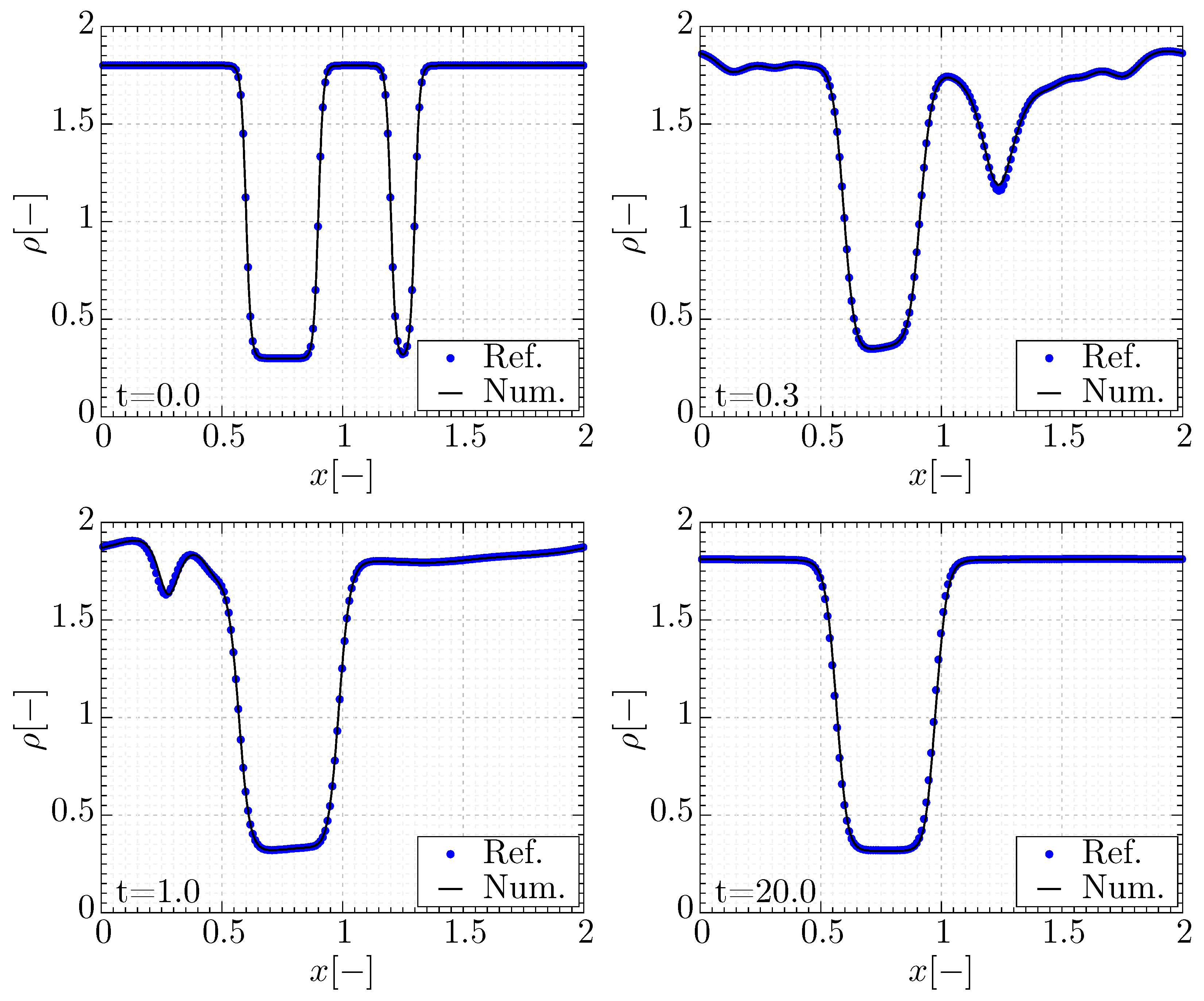
4.1. One-Dimensional Ostwald Ripening

We show a first test case in order to validate the numerical scheme in one dimension of space. Ostwald ripening occurs when a set of different-sized bubbles indirectly merge, without actually moving one towards the other. To summarize the process, smaller bubbles disappear and free their masses into the medium which is absorbed by bigger bubbles. The process continues until one large bubble remains. We consider an initial configuration, adapted from [32,50,53,54,55] described by the following generic initial data

$$\rho (x,0)={\rho }_l+\frac{{\rho }_l-{\rho }_v}{2}\sum _{k=1}^{n_b}\left(\tanh \left(\frac{x-x_k-r_k}{ϵ}\right)-\tanh \left(\frac{x-x_k+r_k}{ϵ}\right)\right),u(x,0)=0,$$

where ${\rho }_l$ represents the initial liquid phase density and ${\rho }_v$ is the initial vapor phase density. $n_b$ is the number of bubbles initially present. For each bubble of index k, $x_k$ is the position of the bubble center and $r_k$ is the approximate radius, so that each bubble spans approximately over the region $[x_k-r_k,x_k+r_k]$. $ϵ$ is a parameter controlling the initial thickness of the `interface’, that is the steepness of the jump from ${\rho }_l$ to ${\rho }_v$ and vice versa. Note that this affects only the transient states as the equilibrium interface width only depends on the capillarity coefficient $\gamma$. For this simulation, we take the same parameters that were used in [32] and which are recalled here for completeness:

$$n_b=2,x_1=0.75,x_2=1.25,r_1=0.15,r_2=0.05,ϵ=0.02,{\rho }_l=1.8,{\rho }_v=0.3,$$

$$\gamma ={10}^{-3},\alpha ={10}^{-2},\beta ={10}^{-5},\mu ={10}^{-2},c_s=10.$$

The computational domain and the corresponding discretization parameters are

$${\mathrm{\Omega }}_c=[0,2],N_x=4096,CFL=0.9.$$

The numerical results are plotted in Figure 3, along the reference numerical solution obtained in [32]. The comparison shows an excellent agreement between both solutions.

4.2. 2D Stationary Droplet

It is possible to compute numerically a quasi-exact stationary solution for the HNSK system in two space dimensions, either by solving an initial value problem or a boundary value problem. We shall use the latter in this case and consider the reference solution computed in [32] using the COLNEW BVP solver, see [81,82,83]. We recall that this solution is obtained from solving the following BVP

$$\left\{\begin{array}{c}{\rho }^{\prime }=\frac{p}{\frac{\eta }{\rho }+\frac{\alpha }{\eta }\rho P^{\prime }\left(\rho \right)},\hfill \\ {\eta }^{\prime }=p,\hfill \\ p^{\prime }=-\frac{p}{r}-\frac{1}{\alpha \gamma \rho }(\rho -\eta ),\hfill \\ \rho (r=0)=1.825,p(r=0)=0,p(r=1)=0.\hfill \end{array}\right.$$

(21)

and is provided for reference in Figure 4. The structure of the solution involves a fast transition separating the liquid and vapor phases and which constitutes the diffuse interface. The peak observed in the gradient field corresponds naturally to the inflection point in the density profile. In order to simulate numerically this solution we take the following parameters

$$\gamma ={10}^{-3},\mu ={10}^{-2},c_s=1,\alpha ={10}^{-2},\beta ={10}^{-3},$$

over different-sized grids. The final time is set to $t=0.025$ and we take $\mathrm{C}\mathrm{F}\mathrm{L}=0.9$. The numerical result is then compared with the initially provided exact solution. A convergence table for this solution is provided in

Table 1. Numerical convergence table for the 2D stationary bubble reference solution obtained from solving (21). $N_x$ and $N_y$ denote the number of elements in the x and y directions. The $L_2$ norm of the errors for a set of representative variables with respect to the exact solution, are reported in the upper part and the corresponding convergence order ${\mathcal{O}}_2$ is reported in the lower one. Parameters used in the simulations are $\gamma ={10}^{-3}$, $\mu ={10}^{-2}$, $c_s=1$, $\alpha ={10}^{-2}$ and $\beta ={10}^{-3}$. Final time is $t=0.025$.

$N_x\times N_y$	${ϵ}_{L_2}\left(\rho \right)$	${ϵ}_{L_2}\left(u\right)$	${ϵ}_{L_2}\left(v\right)$	${ϵ}_{L_2}\left(\eta \right)$	${ϵ}_{L_2}\left(p_1\right)$	${ϵ}_{L_2}\left(p_2\right)$	${ϵ}_{L_2}\left(w\right)$
$64\times 64$	$2.23\times {10}^{-2}$	$2.70\times {10}^{-1}$	$2.70\times {10}^{-1}$	$2.70\times {10}^{-2}$	$8.56\times {10}^{-1}$	$8.56\times {10}^{-1}$	$6.11$
$128\times 128$	$1.32\times {10}^{-2}$	$8.93\times {10}^{-2}$	$8.93\times {10}^{-2}$	$1.31\times {10}^{-2}$	$6.54\times {10}^{-1}$	$6.54\times {10}^{-1}$	$1.88$
$256\times 256$	$4.73\times {10}^{-3}$	$2.02\times {10}^{-2}$	$2.02\times {10}^{-2}$	$4.57\times {10}^{-3}$	$2.07\times {10}^{-1}$	$2.07\times {10}^{-1}$	$4.89\times {10}^{-1}$
$512\times 512$	$1.38\times {10}^{-3}$	$4.99\times {10}^{-3}$	$4.99\times {10}^{-3}$	$1.34\times {10}^{-3}$	$5.16\times {10}^{-2}$	$5.16\times {10}^{-2}$	$1.23\times {10}^{-1}$
$1024\times 1024$	$3.71\times {10}^{-4}$	$1.25\times {10}^{-3}$	$1.25\times {10}^{-3}$	$3.59\times {10}^{-4}$	$1.27\times {10}^{-2}$	$1.27\times {10}^{-2}$	$3.11\times {10}^{-2}$
$N_x\times N_y$	${\mathcal{O}}_{L_2}\left(\rho \right)$	${\mathcal{O}}_{L_2}\left(u\right)$	${\mathcal{O}}_{L_2}\left(v\right)$	${\mathcal{O}}_{L_2}\left(\eta \right)$	${\mathcal{O}}_{L_2}\left(p_1\right)$	${\mathcal{O}}_{L_2}\left(p2\right)$	${\mathcal{O}}_{L_2}\left(w\right)$
$64\times 64$	−	−	−	−	−	−	−
$128\times 128$	$0.76$	$1.60$	$1.60$	$1.04$	$0.39$	$0.39$	$1.70$
$256\times 256$	$1.48$	$2.15$	$2.15$	$1.52$	$1.66$	$1.66$	$1.95$
$512\times 512$	$1.77$	$2.02$	$2.02$	$1.78$	$2.01$	$2.00$	$1.99$
$1024\times 1024$	$1.90$	$1.99$	$1.99$	$1.90$	$2.02$	$2.02$	$1.98$

for a set of variables. The obtained computational results show that our new structure-preserving scheme achieves second-order of accuracy, as expected.

4.3. Non-Condensing Bubble

In order to study quantitatively the numerical curl errors, we consider here a non-condensing 2D bubble. The initial configuration is taken in the form

$$\rho (x,0)={\rho }_l+\frac{{\rho }_l-{\rho }_v}{2}\left(\tanh \left(\frac{r-r_0}{ϵ}\right)-\tanh \left(\frac{r+r_0}{ϵ}\right)\right),u(x,0)=0.$$

(22)

This describes a diffuse bubble centered at the origin with an approximate radius $r_0$. The domain is taken ${\mathrm{\Omega }}_c=[-0.25,0.25]\times [-0.25,0.25]$ discretized over $1024\times 1024$ cells. The remaining physical parameters are taken as follows:

$$r_0=0.10,ϵ=2\sqrt{\gamma },{\rho }_l=1.8,{\rho }_v=0.3,$$

(23a)

$$\gamma =2\times {10}^{-4},\alpha ={10}^{-2},\beta ={10}^{-5},\mu ={10}^{-2},c_s=10.$$

(23b)

The CFL number is set to $CFL=0.9$ and all boundary conditions are periodic. The initial condition is not at equilibrium and the dynamics involve radial fluctuations around the diffuse interface region until a steady state is reached. The time evolution of curl errors is plotted in Figure 5 in two different configurations: one with our new structure-preserving and exactly curl-free discretization, and one without, that is all the variables are simply evolved in the barycenters of the control volumes, using the MUSCL-Hancock-type scheme.

One can clearly see that the discrete curl errors are kept constantly around machine precision when the new compatible and exactly curl-free scheme is used, whereas the curl errors are about eight orders of magnitude higher and growing in time, otherwise. This is a natural consequence of the choice of the grid points used for the computations that ensure such a result for the definition of the proposed discrete curl operator. However, a discrete curl does not have a unique definition. Hence, the following question arises: does the staggered scheme still perform well regarding curl errors when an alternative arbitrary discrete curl definition is employed for a posteriori measuring the curl errors? Thus, let us consider a discrete curl computed by centered finite differences, using barycenter-based values $b^{p,q}$, interpolated a posteriori from the vertices accordingly to (12). This alternative curl in a cell of coordinates $x_p,y_q$, denoted by ${\nabla }_{alt}^h\times {\mathbf{p}}^{p,q}$, reads as

$${\nabla }_{alt}^h\times {\mathbf{p}}^{p,q}=\frac{1}{2}\left(\frac{p_2^{p+1,q}-p_2^{p-1,q}}{\mathrm{\Delta }x}-\frac{p_1^{p,q+1}-p_1^{p,q-1}}{\mathrm{\Delta }y}\right).$$

(24)

We plot hereafter the time evolution of the $L_1$ norm of the discrete curl errors according to the alternative definition (24) and the compatible discrete curl operator (12), for the same parameters reported in (23) and for different mesh sizes. Note that the alternative curl (24) is only used for the postprocessing of the data and for measuring the curl errors. It is not used inside the numerical scheme itself. The obtained computational results are reported in Figure 6.

The results clearly show that for the new structure-preserving finite volume scheme proposed in this paper which is based on the discrete curl ${\nabla }^h\times \mathbf{p}$, for which the method is proven to be exactly curl-free, the curl errors are stable and remain only slightly above machine accuracy, due to round-off errors and which obviously increase with mesh refinement. However, when a simply barycenter-based MUSCL-Hancock method is used, which is not exactly curl-free, the numerical solution becomes unstable and blows up in finite time. The time evolution is thus reported up to the time when this blowup occurs. Similar blowups have been reported previously for hyperbolic PDE with curl involutions in [17,18]. One can observe a significant increase in the curl errors before that happens. On the other hand, for the postprocessing with ${\nabla }_{alt}^h$, it is interesting to observe that even when one changes the definition of the discrete curl operator to an arbitrary one which the method is not meant to preserve exactly, the structure-preserving method still performs much better concerning the curl errors compared to the standard MUSCL-Hancock scheme. The curl errors of the structure-preserving scheme are always lower and essentially do not display any increasing trend and remain bounded over time. In order to investigate the long-time behavior further, which is very important for structure-preserving schemes, we provide in Figure 7 the discrete-curl evolution for the same simulation, but over a longer time for two different meshes. For this simulation, all the model parameters are kept the same as in Figure 6. The figure shows that the discrete curl-errors remain around the machine zero range, even for long times and millions of time steps. The slight increase is of course due to the buildup of round-off errors, which do not necessarily cancel, but which accumulate in time and which are thus naturally greater for more refined meshes.

At this point, it seems also interesting to investigate whether the use of an exactly curl-free scheme has any notable repercussions on the overall behavior of the numerical solution. Thus, we plot in Figure 8 a comparison of the density profile and of the gradient field component $p_1$ for the same non-condensing bubble test, with and without a structure-preserving discretization, at an intermediate time given by $t=2$. The results show that a deformation of the bubble can be observed around the interface region and a glitch can be observed in the center of the bubble when no curl-preservation is in effect. These deformations grow over time and are seemingly what causes the failure of the numerical simulation at later times. To illustrate this further, we also plot the norm of the discrete curl field $|{\nabla }^h\times \mathbf{p}|$ for both simulations in Figure 9. A quick comparison with Figure 8 shows that the curl errors are mainly concentrated around the same locations where the deformations are observed and especially around the middle glitch.

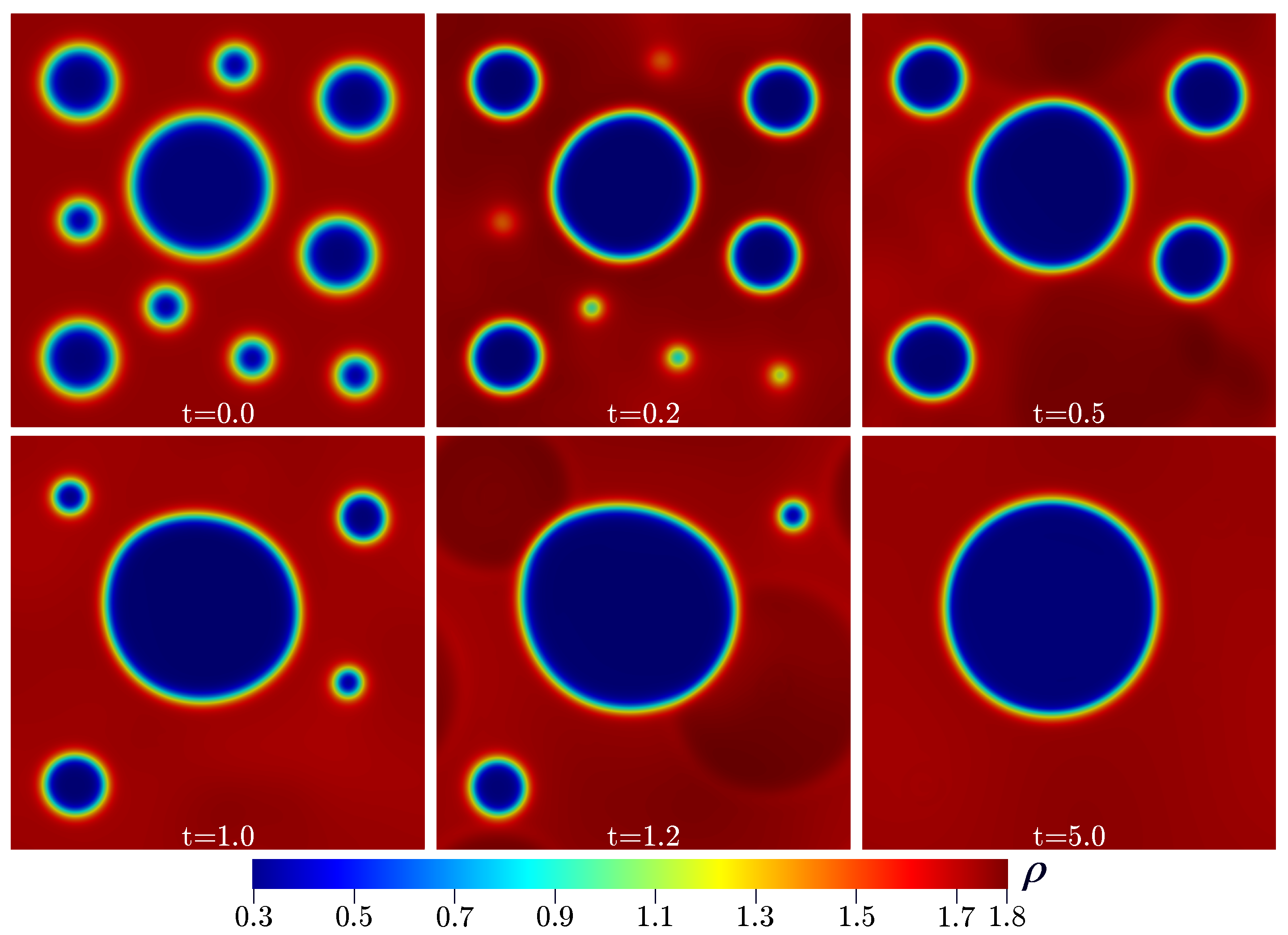
4.4. Two-Dimensional Ostwald Ripening

A standard test case for the NSK system is the 2D Ostwald ripening, see, e.g., [32,50,53,54,55]. The principle and the setting is similar to what is proposed in the one-dimensional counterpart and we consider an initial condition expressed in Cartesian coordinates by the general expression

$$\rho (x,0)={\rho }_l+\frac{{\rho }_l-{\rho }_v}{2}\sum _{k=1}^{n_b}\left(\tanh \left(\frac{c_k-r_k}{ϵ}\right)-\tanh \left(\frac{c_k+r_k}{ϵ}\right)\right),u(x,0)=0,$$

(25)

where the center of the bubble k is located at $(x_k,y_k)$, $c_k$ is the corresponding local radial coordinate $c_k=\sqrt{{(x-x_k)}^2+{(y-y_k)}^2}$ and $r_k$ is the approximate radius of the bubble k. We take here a configuration with $n_b=10$ bubbles, whose initial positions and approximate radii are summarized in

Table 2. Summary of the coordinates and radii of the bubbles in the initial condition (25).

k	1	2	3	4	5	6	7	8	9	10
$x_k$	−0.05	−0.40	−0.40	0.40	0.35	−0.40	0.05	−0.15	0.10	0.40
$y_k$	0.10	−0.40	0.40	0.35	−0.10	−0.00	0.45	−0.25	−0.40	−0.45
$r_k$	0.2	0.10	0.10	0.10	0.10	0.05	0.05	0.05	0.05	0.05

.

Since the dynamics of the solution involve the vanishing of the smaller bubbles and the expansion of the bigger ones, the time evolution involves important topological changes, implying significant dynamics in the order parameters and in the gradient field $\mathbf{p}$. We consider a computational domain ${\mathrm{\Omega }}_c=[-0.6,+0.6]\times [-0.6,+0.6]$ discretized over a grid of $2048\times 2048$ cells. Concerning the parameters we take $ϵ=2\sqrt{\gamma },{\rho }_l=1.8,{\rho }_v=0.3$, $\gamma =2\times {10}^{-4},\alpha ={10}^{-2},\beta ={10}^{-5},\mu ={10}^{-2}$ and $c_s=10$. A CFL number of $0.9$ is used in this simulation. The numerical results are reported in Figure 10 and Figure 11 for the density field $\rho$ and the gradient field $\mathbf{p}$, respectively. The numerical results are qualitatively in accordance with the expected behavior. The solution evolves towards a single bubble configuration equilibrium, after all residual kinetic energy has dissipated.

Figure 11 shows that the gradient field evolved independently, is also qualitatively in agreement with the density field. In order to investigate the results more quantitatively, in particular to check the compatibility of $\rho$ with the order parameter $\eta$ and if the gradient field $\mathbf{p}$ is in line with the gradient of $\eta$, we plot the variables of interest at $t=5$ on the lines defined by $x=-0.05$ and $y=0.1$, both of which cross the final bubble around its center. We compare both $\rho$ and $\eta$ and $\mathbf{p}$ with $\nabla \eta$ computed numerically with finite differences. The comparisons are shown in Figure 12. The results show that the order parameter remains an excellent approximation to the density field. Both components of the independent gradient field $\mathbf{p}$ are also in agreement with the true gradient $\nabla \eta$ in both directions, even after significant deformations occur in the solution.

5. Conclusions

In this paper, we have presented a new second-order accurate exactly curl-free scheme on staggered grids to solve a first-order hyperbolic reformulation of the Navier–Stokes–Korteweg system presented in [32] while also preserving its natural curl involution constraints exactly at the discrete level. The tests in two dimensions of space show that the discrete curl errors remain around machine precision and are stable in time. We also showed that in the absence of an exactly curl-free discretization, erroneous behaviors can be observed in the solution, leading to finite-time blowups, especially for under-resolved meshes.

Future research will concern the extension to three space dimensions, which is out of scope of the present paper. Another future direction of research would be to improve the current scheme by a semi-implicit time discretization, similar to the one forwarded in [17,74,77]. This requires first to find an appropriate splitting of the hyperbolic system, allowing to separate the fast relaxation characteristics so that a semi-implicit discretization would improve the overall performance and reduce the time-stepping constraints. The development of arbitrary high-order structure preserving methods is also considered on the longer term, following the ideas presented in [84,85]. Future work will also concern the extension of the presented exactly curl-free discretization to a thermodynamically compatible one, similar to the ideas on HTC schemes recently presented in [86,87,88]. The framework of HTC schemes allows the construction of provably nonlinearly stable schemes in the energy norm and to the best of our knowledge, there are no exactly curl-free HTC schemes available yet. To date, in HTC schemes the involution constraints have been taken into account via a hyperbolic and thermodynamically compatible GLM cleaning approach, see, e.g., [89].

References

1. Klainermann, S.; Majda, A. Singular Limits of Quasilinear Hyperbolic Systems with Large Parameters and the Incompressible Limit of Compressible Fluid. Comm. Pure Appl. Math. 1981, 34, 481–524. [Google Scholar] [CrossRef]
2. Klainermann, S.; Majda, A. Compressible and incompressible fluids. Commun. Pure Appl. Math. 1982, 35, 629–651. [Google Scholar] [CrossRef]
3. Munz, C.; Klein, R.; Roller, S.; Geratz, K. The extension of incompressible flow solvers to the weakly compressible regime. Comput. Fluids 2003, 32, 173–196. [Google Scholar] [CrossRef]
4. Godunov, S.; Romenski, E. Nonstationary equations of the nonlinear theory of elasticity in Euler coordinates. J. Appl. Mech. Tech. Phys. 1972, 13, 868–885. [Google Scholar] [CrossRef]
5. Romenski, E. Hyperbolic systems of thermodynamically compatible conservation laws in continuum mechanics. Math. Comput. Model. 1998, 28, 115–130. [Google Scholar] [CrossRef]
6. Dumbser, M.; Peshkov, I.; Romenski, E.; Zanotti, O. High order ADER schemes for a unified first order hyperbolic formulation of continuum mechanics: Viscous heat-conducting fluids and elastic solids. J. Comput. Phys. 2016, 314, 824–862. [Google Scholar] [CrossRef]
7. Peshkov, I.; Romenski, E. A hyperbolic model for viscous Newtonian flows. Contin. Mech. Thermodyn. 2016, 28, 85–104. [Google Scholar] [CrossRef]
8. Godunov, S.; Romenski, E. Elements of Continuum Mechanics and Conservation Laws; Kluwer Academic/Plenum Publishers: Dordrecht, The Netherlands, 2003. [Google Scholar]
9. Peshkov, I.; Pavelka, M.; Romenski, E.; Grmela, M. Continuum mechanics and thermodynamics in the Hamilton and the Godunov-type formulations. Contin. Mech. Thermodyn. 2018, 30, 1343–1378. [Google Scholar] [CrossRef]
10. Romenski, E.; Drikakis, D.; Toro, E. Conservative models and numerical methods for compressible two-phase flow. J. Sci. Comput. 2010, 42, 68–95. [Google Scholar] [CrossRef]
11. Alic, D.; Bona, C.; Bona-Casas, C. Towards a gauge-polyvalent numerical relativity code. Phys. Rev. D 2009, 79, 044026. [Google Scholar] [CrossRef] [Green Version]
12. Brown, J.D.; Diener, P.; Field, S.E.; Hesthaven, J.S.; Herrmann, F.; Mroué, A.H.; Sarbach, O.; Schnetter, E.; Tiglio, M.; Wagman, M. Numerical simulations with a first-order BSSN formulation of Einstein’s field equations. Phys. Rev. D 2012, 85, 084004. [Google Scholar] [CrossRef]
13. Dumbser, M.; Fambri, F.; Gaburro, E.; Reinarz, A. On GLM curl cleaning for a first order reduction of the CCZ4 formulation of the Einstein field equations. J. Comput. Phys. 2020, 404, 109088. [Google Scholar] [CrossRef]
14. Brackbill, J.U.; Barnes, D.C. The Effect of Nonzero div(B) on the numerical solution of the magnetohydrodynamic equations. J. Comput. Phys. 1980, 35, 426–430. [Google Scholar] [CrossRef]
15. Brackbill, J. Fluid modeling of magnetized plasmas. Space Sci. Rev. 1985, 42, 153–167. [Google Scholar] [CrossRef]
16. Balsara, D.; Spicer, D. A Staggered Mesh Algorithm Using High Order Godunov Fluxes to Ensure Solenoidal Magnetic Fields in Magnetohydrodynamic Simulations. J. Comput. Phys. 1999, 149, 270–292. [Google Scholar] [CrossRef]
17. Chiocchetti, S.; Dumbser, M. An exactly curl-free staggered semi-implicit finite volume scheme for a first order hyperbolic model of viscous flow with surface tension. J. Sci. Comput. 2023, 94, 24. [Google Scholar] [CrossRef]
18. Chiocchetti, S.; Peshkov, I.; Gavrilyuk, S.; Dumbser, M. High order ADER schemes and GLM curl cleaning for a first order hyperbolic formulation of compressible flow with surface tension. J. Comput. Phys. 2021, 426, 109898. [Google Scholar] [CrossRef]
19. Yee, K. Numerical solution of initial boundary value problems involving Maxwell’s equations in isotropic media. IEEE Trans. Antennas Propag. 1966, 14, 302–307. [Google Scholar]
20. Holland, R. Finite-difference solution of Maxwell’s equations in generalized nonorthogonal coordinates. IEEE Trans. Nucl. Sci. 1983, 30, 4589–4591. [Google Scholar] [CrossRef]
21. Brecht, S.; Lyon, J.; Fedder, J.; Hain, K. A simulation study of east–west IMF effects on the magnetosphere. Geophys. Res. Lett. 1981, 8, 397–400. [Google Scholar] [CrossRef]
22. Evans, C.R.; Hawley, J.F. Simulation of magnetohydrodynamic flows-A constrained transport method. Astrophys. J. 1988, 332, 659–677. [Google Scholar] [CrossRef]
23. DeVore, C.R. Flux-corrected transport techniques for multidimensional compressible magnetohydrodynamics. J. Comput. Phys. 1991, 92, 142–160. [Google Scholar] [CrossRef]
24. Dai, W.; Woodward, P.R. A simple finite difference scheme for multidimensional magnetohydrodynamical equations. J. Comput. Phys. 1998, 142, 331–369. [Google Scholar] [CrossRef]
25. Tóth, G. The ∇ · B = 0 constraint in shock-capturing magnetohydrodynamics codes. J. Comput. Phys. 2000, 161, 605–652. [Google Scholar] [CrossRef]
26. Gardiner, T.A.; Stone, J.M. An unsplit Godunov method for ideal MHD via constrained transport. J. Comput. Phys. 2005, 205, 509–539. [Google Scholar] [CrossRef]
27. Munz, C.; Omnes, P.; Schneider, R.; Sonnendrücker, E.; Voss, U. Divergence Correction Techniques for Maxwell Solvers Based on a Hyperbolic Model. J. Comput. Phys. 2000, 161, 484–511. [Google Scholar] [CrossRef]
28. Dedner, A.; Kemm, F.; Kröner, D.; Munz, C.D.; Schnitzer, T.; Wesenberg, M. Hyperbolic Divergence Cleaning for the MHD Equations. J. Comput. Phys. 2002, 175, 645–673. [Google Scholar] [CrossRef]
29. Dedner, A.; Rohde, C.; Wesenberg, M. A new approach to divergence cleaning in magnetohydrodynamic simulations. In Hyperbolic Problems: Theory, Numerics, Applications; Springer: New York, NY, USA, 2003; pp. 509–518. [Google Scholar]
30. Jacobs, G.; Hesthaven, J.S. Implicit–explicit time integration of a high-order particle-in-cell method with hyperbolic divergence cleaning. Comput. Phys. Commun. 2009, 180, 1760–1767. [Google Scholar] [CrossRef]
31. Busto, S.; Dumbser, M.; Escalante, C.; Gavrilyuk, S.; Favrie, N. On high order ADER discontinuous Galerkin schemes for first order hyperbolic reformulations of nonlinear dispersive systems. J. Sci. Comput. 2021, 87, 48. [Google Scholar] [CrossRef]
32. Dhaouadi, F.; Dumbser, M. A first order hyperbolic reformulation of the Navier–Stokes-Korteweg system based on the GPR model and an augmented Lagrangian approach. J. Comput. Phys. 2022, 470, 111544. [Google Scholar] [CrossRef]
33. Balsara, D. Second-Order Accurate Schemes for Magnetohydrodynamics with Divergence-Free Reconstruction. Astrophys. J. Suppl. Ser. 2004, 151, 149–184. [Google Scholar] [CrossRef]
34. Xu, Z.; Balsara, D.S.; Du, H. Divergence-free WENO reconstruction-based finite volume scheme for solving ideal MHD equations on triangular meshes. Commun. Comput. Phys. 2016, 19, 841–880. [Google Scholar] [CrossRef]
35. Hazra, A.; Chandrashekar, P.; Balsara, D.S. Globally constraint-preserving FR/DG scheme for Maxwell’s equations at all orders. J. Comput. Phys. 2019, 394, 298–328. [Google Scholar] [CrossRef]
36. Balsara, D.S.; Simpson, J.J. Making a synthesis of FDTD and DGTD schemes for computational electromagnetics. IEEE J. Multiscale Multiphysics Comput. Tech. 2020, 5, 99–118. [Google Scholar] [CrossRef]
37. Balsara, D.; Käppeli, R.; Boscheri, W.; Dumbser, M. Curl constraint-preserving reconstruction and the guidance it gives for mimetic scheme design. Commun. Appl. Math. Comput. Sci. 2021, 1–60. [Google Scholar] [CrossRef]
38. Audiard, C.; Haspot, B. Global well-posedness of the Euler–Korteweg system for small irrotational data. Commun. Math. Phys. 2017, 351, 201–247. [Google Scholar] [CrossRef]
39. Benzoni-Gavage, S. Planar traveling waves in capillary fluids. Differ. Integral Equ. 2013, 26, 439–485. [Google Scholar] [CrossRef]
40. Benzoni-Gavage, S.; Danchin, R.; Descombes, S. On the well-posedness for the Euler–Korteweg model in several space dimensions. Indiana Univ. Math. J. 2007, 56, 1499–1580. [Google Scholar] [CrossRef]
41. Benzoni-Gavage, S.; Descombes, S.; Jamet, D.; Mazet, L. Structure of Korteweg models and stability of diffuse interfaces. Interfaces Free Boundaries 2005, 7, 371–414. [Google Scholar] [CrossRef]
42. Bresch, D.; Gisclon, M.; Lacroix-Violet, I. On Navier–Stokes–Korteweg and Euler–Korteweg systems: Application to quantum fluids models. Arch. Ration. Mech. Anal. 2019, 233, 975–1025. [Google Scholar] [CrossRef]
43. Bresch, D.; Couderc, F.; Noble, P.; Vila, J.P. New extended formulations of euler-korteweg equations based on a generalization of the quantum bohm identity. arXiv 2015, arXiv:1503.08678. [Google Scholar]
44. Bresch, D.; Couderc, F.; Noble, P.; Vila, J. A generalization of the quantum Bohm identity: Hyperbolic CFL condition for Euler–Korteweg equations. Comptes Rendus Math. 2016, 354, 39–43. [Google Scholar] [CrossRef] [Green Version]
45. Casal, P.; Gouin, H. A representation of liquid-vapor interfaces by using fluids of second grade. Annales de Physique 1988, 13, 3–12. [Google Scholar]
46. Gavrilyuk, S.L.; Shugrin, S.M. Media With Equations of State That Depend on derivatives. J. Appl. Mech. Tech. Phys. 1996, 37, 177–189. [Google Scholar] [CrossRef]
47. Haspot, B. Existence of strong solutions for nonisothermal Korteweg system. Ann. MathÉMatiques Blaise Pascal 2009, 16, 431–481. [Google Scholar] [CrossRef]
48. Noble, P.; Vila, J. Stability theory for difference approximations of some dispersive shallow water equations and application to thin film flows. arXiv 2013, arXiv:1304.3805. [Google Scholar]
49. Anderson, D.; McFadden, G.; Wheeler, A. Diffuse-interface methods in fluid mechanics. Annu. Rev. Fluid Mech. 1998, 30, 139–165. [Google Scholar] [CrossRef]
50. Diehl, D.; Kremser, J.; Kröner, D.; Rohde, C. Numerical solution of Navier–Stokes-Korteweg systems by Local Discontinuous Galerkin methods in multiple space dimensions. Appl. Math. Comput. 2016, 272, 309–335. [Google Scholar] [CrossRef]
51. Rohde, C. A local and low-order Navier–Stokes–Korteweg system. Nonlinear Part. Differ. Equ. Hyperbolic Wave Phenom. 2010, 526, 315–337. [Google Scholar]
52. Corli, A.; Rohde, C.; Schleper, V. Parabolic approximations of diffusive–dispersive equations. J. Math. Anal. Appl. 2014, 414, 773–798. [Google Scholar] [CrossRef]
53. Neusser, J.; Rohde, C.; Schleper, V. Relaxation of the Navier–Stokes–Korteweg equations for compressible two-phase flow with phase transition. Int. J. Numer. Methods Fluids 2015, 79, 615–639. [Google Scholar] [CrossRef]
54. Chertock, A.; Degond, P.; Neusser, J. An asymptotic-preserving method for a relaxation of the Navier–Stokes–Korteweg equations. J. Comput. Phys. 2017, 335, 387–403. [Google Scholar] [CrossRef]
55. Hitz, T.; Keim, J.; Munz, C.; Rohde, C. A parabolic relaxation model for the Navier–Stokes-Korteweg equations. J. Comput. Phys. 2020, 421, 109714. [Google Scholar] [CrossRef]
56. Keim, J.; Munz, C.D.; Rohde, C. A Relaxation Model for the Non-Isothermal Navier–Stokes-Korteweg Equations in Confined Domains. J. Comput. Phys. 2022. submitted. [Google Scholar] [CrossRef]
57. Kapila, A.; Menikoff, R.; Bdzil, J.; Son, S.; Stewart, D. Two-phase modelling of DDT in granular materials: Reduced equations. Phys. Fluids 2001, 13, 3002–3024. [Google Scholar] [CrossRef]
58. Andrianov, N.; Warnecke, G. The Riemann problem for the Baer–Nunziato two-phase flow model. J. Comput. Phys. 2004, 212, 434–464. [Google Scholar] [CrossRef]
59. Saurel, R.; Abgrall, R. A Multiphase Godunov Method for Compressible Multifluid and Multiphase Flows. J. Comput. Phys. 1999, 150, 425–467. [Google Scholar] [CrossRef]
60. Abgrall, R.; Saurel, R. Discrete equations for physical and numerical compressible multiphase mixtures. J. Comput. Phys. 2003, 186, 361–396. [Google Scholar] [CrossRef]
61. Favrie, N.; Gavrilyuk, S. Diffuse interface model for compressible fluid - Compressible elastic-plastic solid interaction. J. Comput. Phys. 2012, 231, 2695–2723. [Google Scholar] [CrossRef]
62. Ndanou, S.; Favrie, N.; Gavrilyuk, S. Multi–solid and multi–fluid diffuse interface model: Applications to dynamic fracture and fragmentation. J. Comput. Phys. 2015, 295, 523–555. [Google Scholar] [CrossRef]
63. Favrie, N.; Gavrilyuk, S.; Saurel, R. Solid–fluid diffuse interface model in cases of extreme deformations. J. Comput. Phys. 2009, 228, 6037–6077. [Google Scholar] [CrossRef]
64. de Brauer, A.; Iollo, A.; Milcent, T. A Cartesian Scheme for Compressible Multimaterial Hyperelastic Models with Plasticity. Commun. Comput. Phys. 2017, 22, 1362–1384. [Google Scholar] [CrossRef]
65. Barton, P.T. An interface-capturing Godunov method for the simulation of compressible solid-fluid problems. J. Comput. Phys. 2019, 390, 25–50. [Google Scholar] [CrossRef]
66. De Lorenzo, M.; Pelanti, M.; Lafon, P. HLLC-type and path-conservative schemes for a single–velocity six-equation two-phase flow model: A comparative study. Appl. Math. Comput. 2018, 333, 95–117. [Google Scholar] [CrossRef]
67. Kemm, F.; Gaburro, E.; Thein, F.; Dumbser, M. A simple diffuse interface approach for compressible flows around moving solids of arbitrary shape based on a reduced Baer-Nunziato model. Comput. Fluids 2020, 204, 104536. [Google Scholar] [CrossRef] [Green Version]
68. Re, B.; Abgrall, R. A pressure-based method for weakly compressible two-phase flows under a Baer–Nunziato type model with generic equations of state and pressure and velocity disequilibrium. Int. J. Numer. Methods Fluids 2022, 94, 1183–1232. [Google Scholar] [CrossRef]
69. Thein, F.; Romenski, E.; Dumbser, M. Exact and numerical solutions of the Riemann problem for a conservative model of compressible two-phase flows. J. Sci. Comput. 2022, 93, 83. [Google Scholar] [CrossRef]
70. Lukácová-Medvidóvá, M.; Puppo, G.; Thomann, A. An all Mach number finite volume method for isentropic two-phase flow. J. Numer. Math. 2023, in press. [Google Scholar] [CrossRef]
71. Dhaouadi, F.; Favrie, N.; Gavrilyuk, S. Extended Lagrangian approach for the defocusing nonlinear Schrödinger equation. Stud. Appl. Math. 2019, 142, 336–358. [Google Scholar] [CrossRef]
72. Dhaouadi, F.; Gavrilyuk, S.; Vila, J.P. Hyperbolic relaxation models for thin films down an inclined plane. Appl. Math. Comput. 2022, 433, 127378. [Google Scholar] [CrossRef]
73. Dhaouadi, F. An augmented lagrangian Approach for Euler–Korteweg Type Equations. Ph.D. Thesis, Université Paul Sabatier-Toulouse III, Toulouse, France, 2020. [Google Scholar]
74. Boscheri, W.; Dumbser, M.; Ioriatti, M.; Peshkov, I.; Romenski, E. A structure-preserving staggered semi-implicit finite volume scheme for continuum mechanics. J. Comput. Phys. 2010, 424, 109866. [Google Scholar] [CrossRef]
75. Balsara, D. A two-dimensional HLLC Riemann solver for conservation laws: Application to Euler and magnetohydrodynamic flows. J. Comput. Phys. 2012, 231, 7476–7503. [Google Scholar] [CrossRef]
76. Balsara, D. Multidimensional Riemann problem with self-similar internal structure—Part I—Application to hyperbolic conservation laws on structured meshes. J. Comput. Phys. 2014, 277, 163–200. [Google Scholar] [CrossRef]
77. Dumbser, M.; Balsara, D.S.; Tavelli, M.; Fambri, F. A divergence-free semi-implicit finite volume scheme for ideal, viscous and resistive magnetohydrodynamics. Int. J. Numer. Methods Fluids 2019, 89, 16–42. [Google Scholar] [CrossRef]
78. van der Waals, J.D. The thermodynamic theory of capillarity under the hypothesis of a continuous variation of density. J. Stat. Phys. 1979, 20, 200–244. [Google Scholar] [CrossRef]
79. van der Waals, J.D. Over de Continuiteit van den Gas- en Vloei Stof Toestand. Ph.D. Thesis, University of Leiden, South Holland, The Netherlands, 1873. [Google Scholar]
80. Toro, E. Riemann Solvers and Numerical Methods for Fluid Dynamics, 2nd ed.; Springer: New York, NY, USA, 1999. [Google Scholar]
81. Ascher, U.; Christiansen, J.; Russell, R. A collocation solver for mixed order systems of boundary value problems. Math. Comput. 1979, 33, 659–679. [Google Scholar] [CrossRef]
82. Ascher, U.; Christiansen, J.; Russell, R. Collocation software for boundary-value ODEs. ACM Trans. Math. Softw. (TOMS) 1981, 7, 209–222. [Google Scholar] [CrossRef]
83. Bader, G.; Ascher, U. A new basis implementation for a mixed order boundary value ODE solver. SIAM J. Sci. Stat. Comput. 1987, 8, 483–500. [Google Scholar] [CrossRef]
84. Tavelli, M.; Dumbser, M. A pressure-based semi-implicit space-time discontinuous Galerkin method on staggered unstructured meshes for the solution of the compressible Navier–Stokes equations at all Mach numbers. J. Comput. Phys. 2017, 341, 341–376. [Google Scholar] [CrossRef]
85. Fambri, F.; Dumbser, M. Semi-implicit discontinuous Galerkin methods for the incompressible Navier-Stokes equations on adaptive staggered Cartesian grids. Comput. Methods Appl. Mech. Eng. 2017, 324, 170–203. [Google Scholar] [CrossRef]
86. Busto, S.; Dumbser, M.; Peshkov, I.; Romenski, E. On thermodynamically compatible finite volume schemes for continuum mechanics. SIAM J. Sci. Comput. 2022, 44, A1723–A1751. [Google Scholar] [CrossRef]
87. Abgrall, R.; Busto, S.; Dumbser, M. A simple and general framework for the construction of thermodynamically compatible schemes for computational fluid and solid mechanics. Appl. Math. Comput. 2023, 440, 127629. [Google Scholar] [CrossRef]
88. Gaburro, E.; Öffner, P.; Ricchiuto, M.; Torlo, D. High order entropy preserving ADER-DG schemes. Appl. Math. Comput. 2023, 440, 127644. [Google Scholar] [CrossRef]
89. Busto, S.; Dumbser, M. A new thermodynamically compatible finite volume scheme for magnetohydrodynamics. SIAM J. Numer. Anal. 2023, in press. [Google Scholar] [CrossRef]
Figure 1. The Van der Waals pressure as a function of ρ for the values given in (4). ρ V M and ρ L M are the Maxwell states for the vapor and liquid phases, respectively. ρ V * and ρ L * are local extrema of the pressure and delimit the non-convexity region.
Mathematics 11 00876 g001
Figure 2. Schematic of the computational domain featuring the grid points and the staggered dual grid points. Red squares are barycenters and blue circles are the vertexes of the computational cells.
Mathematics 11 00876 g002
Figure 3. Density profile for the 1D Ostwald ripening simulation plotted at four different times t { 0 , 0.3 , 1 , 20 } obtained by our scheme (Num, black line) and compared against a reference numerical solution (Ref, blue dots) obtained using an ADER-DG P 3 P 3 method presented in [32]. Parameters used for this simulation are γ = 10 3 , μ = 10 2 , c s = 10 , α = 10 2 and β = 10 5 . The domain is discretized over N x = 4096 cells.
Mathematics 11 00876 g003
Figure 4. Boundary value problem reference solution for the HNSK system. The left figure shows the radial profiles of ρ and η while the right one shows the radial profile of the gradient field, for α = 10 2 and γ = 10 3 .
Mathematics 11 00876 g004
Figure 5. Time-evolution of the L 2 norm of the discrete curl errors when a staggered compatible curl-free discretization is used (blue) and when no staggering is in effect (orange), for the non-condensing bubble test case. For both simulations, the parameters are γ = 2 × 10 4 , α = 10 2 , β = 10 5 , μ = 10 2 , c s = 10 . The computational domain is Ω c = [ 0.25 , 0.25 ] × [ 0.25 , 0.25 ] discretized over 1024 × 1024 cells.
Mathematics 11 00876 g005
Figure 6. Time-evolution of the L 1 norm of the discrete curl errors, with both h (left) and a l t h (right), when the structure-preserving (SP, continuous lines) staggered scheme is used versus a simple MUSCL-Hancock (MH, dashed lines) method , on different mesh sizes for the non-condensing bubble test case. The parameters are γ = 2 × 10 4 , α = 10 2 , β = 10 5 , μ = 10 2 , c s = 10 . The computational domain is Ω c = [ 0.25 , 0.25 ] × [ 0.25 , 0.25 ] .
Mathematics 11 00876 g006
Figure 7. Long-term evolution of the discrete curl errors, for the non-condensing bubble test case. The left figure corresponds to a simulation with a 512 × 512 grid, while the right figure is for a 128 × 128 grid. The model parameters taken here are the same as in Figure 6. The upper horizontal axis indicates the number of time steps, while the lower axis reports the time t.
Mathematics 11 00876 g007
Figure 8. Comparison of the overall shape of the density field ρ (top) and the gradient field component p 1 (bottom) with both a curl-free discretization (left) and without (right). Results are shown for t = 2 on the 512 × 512 grid.
Mathematics 11 00876 g008
Figure 9. Two-dimensional distribution of the curl errors | h × p | over the full computational domain for both schemes, for the same non-condensing bubble simulation over the 512 × 512 grid.
Mathematics 11 00876 g009
Figure 10. Numerical result for the density ρ , obtained by our curl-free scheme for the two-dimensional Ostwald ripening test case. Results are plotted at times t { 0 , 0.2 , 0.5 , 1.0 , 1.2 , 5.0 } . We recall that the values used here are ρ l = 1.8 , ρ v = 0.3 , γ = 2 × 10 4 , α = 10 2 , β = 10 5 , c s = 10 and an effective viscosity of μ = 10 2 . The total domain is Ω = [ 0.6 , + 0.6 ] × [ 0.6 , + 0.6 ] discretized over a 4096 × 4096 uniform grid with periodic boundary conditions.
Mathematics 11 00876 g010
Figure 11. Numerical result for the magnitude of the gradient field p for the same simulation as in Figure 10.
Mathematics 11 00876 g011
Figure 12. Comparison of the density profile with the order parameter η (top) and of the gradient field components p 1 and p 2 with x h ( η ) and y h ( η ) , respectively, computed with finite differences. The comparison is made at t = 5 , on two extracted lines from the results of Figure 10 and Figure 11, defined by y = 0.1 (left) and x = 0.05 (right).
Mathematics 11 00876 g012