Abstract
The second-order system of non-stiff Initial Value Problems (IVP) is considered and, in particular, the case where the first derivatives are absent. This kind of problem is interesting since since it arises in many significant problems, e.g., in Celestial mechanics. Runge–Kutta–Nyström (RKN) pairs are perhaps the most successful approaches for solving such type of IVPs. To achieve a pair attaining orders eight and six, we have to solve a well-defined set of equations with respect to the coefficients. Here, we provide a simplified form of these equations in a robust algorithm. When creating such pairings for use in double precision arithmetic, numerous conditions are often satisfied. First and foremost, we strive to keep the coefficients’ magnitudes small to prevent accuracy loss. We may, however, allow greater coefficients when working with quadruple precision. Then, we may build pairs of orders eight and six with significantly smaller truncation errors. In this paper, a novel pair is generated that, as predicted, outperforms state-of-the-art pairs of the same orders in a collection of important problems.
MSC:
65L05; 65L06
1. Introduction
Second order initial value problems (IVP) of the specific form
with sufficiently continuous differentiable and is considered here.
We evaluate an approximation to the solution of problem (1) at a set of distinct points using an explicit Runge–Kutta–Nyström method of algebraic order p. This method’s format is as follows (see [1] and ([2], p. 283) for further explanations on these methods):
where is the size of the step. The last 50 years have seen a persistent interest in these methods. Follow the works of E. Fehlberg [3], Dormand et al. [4,5], El-Mikkawy and Rahmo [6], Papakostas et al. [7], Simos et al. [8], and Jerbi et al. [9]. There have also been RKN methods presented with special features. Houven et al. investigated RKN methods with lower phase lags, while Yoshida [10] and Calvo et al. [11] built RKN algorithms with the symplectic property.
In this paper, we set and we combine the aforementioned method with an additional formula of order six. In light of this, we also calculate an estimate of fifth order using the same values of ,
The higher order approximations are employed in all circumstances to propagate the solutions in time.
As a result, we have an estimator of error
Then, we compare with which is a small positive number defined by the user. Then, using this little value, known as tolerance, we can estimate the length of the following step as
which is in common use for the RKN8(6) pairs [4,12]. When , we prevent the solution from propagating. We essentially repeat the current step, but this time we use as the new shorter version rather than .
The Butcher tableau may be used to represent the coefficients [13]. As a result, the method appears in the form
with , i.e. the weights are represented as row vectors.
Below we take into account a triplet with nine stages (). The Butcher tableau shown in Table 1 displays its coefficients.

Table 1.
The Butcher tableau of RKN pairs of orders 8(6).
Using such a method, we spend only eight stages per step since the final stage is reused as first stage in the following step. Thus, the numbers in the ninth stage coincide with w, i.e., for . This technique is known as FSAL (First Stage As Last).
RKN pairs of orders eight and six that use effectively eight stages per step were studied in [5,7]. Eighth order RKN methods that share seven stages per step have only been constructed for the special case of linear inhomogeneous problems [14].
2. Runge–Kutta–Nyström Methods of Eighth Order
We apply a RKN method to (1) and deploy the Taylor series expansions for and . When matching expressions up to for an eighth order method, the following results are obtained:
where are expressions depending on while are expressions depending on . An algorithm for their symbolic derivation of is given in [15]. Expressions are elementary differentials with respect to and its partial derivatives. The elementary differentials come from the problem and can not be handled by the method. However, for an eighth order RKN method we have to eliminate the coefficients and in expressions (3) and (4) to the requested order. In Table 2, we list the number of order conditions (i.e., of and ) for each order. Thus, e.g., for a third algebraic order method we have to nullify equations for and another order conditions for .
Table 2.
Number of equations of conditions for RKN methods.
Inspecting from Butcher tableau above (i.e., Table 1) the number of coefficients available for a nine stages method and compared it with the equations of condition up to eighth order as reported in Table 2, we see that are far too less. Thus, we proceed making various simplifying assumptions that drastically reduce the number of order conditions. Firstly, we set
with the identity matrix and . Using this assumption we automatically satisfy the order conditions for after eliminating the equations of the same order for . Then, we are interested in eliminating only with respect to .
Again summing the numbers in the last row of Table 2, we see that are remaining to too many for the coefficients at hand. Thus, we proceed making the following assumptions
with
the componentwise multiplication among matrices (i.e., Hadamard multiplication), while . This multiplication has lower priority than dot product.
We also consider the row simplifying condition for RKN methods
and the subsidiary simplifying assumptions
Then we achieve a severe reduction in the number of order conditions and we may continue deriving the coefficients of an eighth order method (i.e., and c) by the following algorithm.
- BEGIN ALGORITHM
Select arbitrary values for the coefficients and .
Then compute successively and explicitly
Solve Vandermonde equations
for . The last Vandermonde equation is automatically satisfied by the selection of . Then vector w comes explicitly from (5).
Solve , for and . Notice here that is a vector and, thus, is its fourth component.
Solve , ans for .
Solve the following three integral equations
for .
Evaluate from , for .
Evaluate from and its respective coordinates.
In the end we get
and
- END OF ALGORITHM
It is of interest to remark that no such simplified algorithm has ever appeared until now. It helped us very much in deriving our triplet.
3. Producing a RKN Pair of Orders 8 and 6
By the algorithm given in the previous section we may construct an eighth order RKN method at an actual cost of eight stages per step. This algorithm is that it offers six free parameters. Thus, we may exploit them in order to improve the efficiency of our new method. We choose to minimize the terms of the principal error terms, i.e., the Euclidean norm of the ninth order coefficients and , that appear in series expansions (3) and (4).
When utilizing double precision arithmetic, we traditionally aim to keep the magnitude of the coefficients as small as possible. The margins of the available digits would therefore be severely tested by a coefficient of size , a function value of size and a tolerance of . However, with quadruple precision, we are still able to accept these large coefficients with tolerances as low as approximately . By allowing the coefficients to increase, we can now move on to a new minimization procedure.
In order to address this, we choose to use Differential Evolution Algorithm [16,17]. Differential Evolution is an iterative procedure and in every iteration, named generation g, we work with a “population” of individuals , with P the population size. An initial population , is randomly created in the first step of the method. We have also set as fitness function the expression
which measures the loss from a ninth order method. The fitness function is then evaluated for each individual in the initial population and it is meant to be minimized. A three-phase sequential procedure updates every participant in each generation (iteration) g. The stages are Differentiation, Crossover, and Selection. We used the software DeMat [18] in MATLAB [19] where the latter technique is implemented. Success is not guaranteed with one optimization. Thus, we run the procedure several hundred times. Then we manage to get a solution. The result is further refined in order to get more digits of accuracy. This was done working on multi-precision arithmetic and using the function NMinimize of Mathematica [20].
The main characteristics of the major RKN pairs of eighth order studied here are given in Table 3. The norms presented there correspond to the Euclidean norm of the coefficients ninth order (i.e., of ) in the expressions (3) and (4). We expect the new method to perform better since it produces significantly reduced local truncation errors.
Table 3.
Basic characteristics of the RKN pairs considered.
The coefficients of the method constructed can be found in the following Mathematica module where we also implemented the integration algorithm we used in numerical tests in Listing 1.
| Listing 1.Mathematica Module implementing the new pair. |
RKNT86[f_List, vars_List, initialvalues_List, dinitialvalues_List,
finalx_, errorTolerance_] :=
Block[{x = SetAccuracy[First[initialvalues], 33],
y = SetAccuracy[Rest[initialvalues], 33], dy = SetAccuracy[dinitialvalues, 33],
xend = SetAccuracy[finalx, 33], h, err, hnew, y7, y8, dy7, dy8, solution, hmax,
ireject, k = Table[i + j, {i, 9}, {j, Length[vars] - 1}],
b=SetAccuracy[{46704396222138759/1124501888012545693,0,
84069894477030747/424535379079037893,60269691739898297/328032958547368465,
2009963068113133/27794099874007722,162341471393132/140140455957185117,
6086576956589044/1882413506280312633,0,0},33],
bb=SetAccuracy[{10769958754260247/261191895425614637,0,
104933541030533329/527807735255158343,8187542127950603/44863180380403502,
50493885750265423/674323734860213804,-396215365808089/252398506959352750,
5468871271464350/1319483122963052413,0,0},33],
db=SetAccuracy[{46704396222138759/1124501888012545693,0,
90371972523959954/390135632629351589,118990880894033457/367654647557162744,
180830119624415039/624884373647391279,16628088200566168/1643600751401035359,
1524820183138666476/417332398303375801,-942444174868320016/265473221553563103,
0},33],
dbb=SetAccuracy[{10769958754260247/261191895425614637,0,
58861559987617091/253105545276009947,142913350550568712/444546485690175277,
8398007711885933/28026591338889651,-8440103966850896/615634893567208211,
1592393294195924241/339999309740023022,
-6699802037196600096/1421037300124099357,3/20},33],
c=SetAccuracy[{0,8065253268/111157879849,16130506536/111157879849,99/229,
1855/2473,116/131,1129/1130,1,1},33],
a=SetAccuracy[{{0},{502615833312847/190946037812928939},
{1601030787675953/456179150746555700,1601030787675953/228089575373277850},
{47478115875661981/518814108724307373,-64883723802385428/357040639400014459,
25666007926449694/139746227660637731},
{-328112826298039228/251912779790891183,969895830706346953/297412056373654755,
-958305119264262743/492487831928632961,151603443293999467/564549369158251216},
{44079989458325648760/345626831710945999,-267609305840442666747/859338149021870938,
130442442641184422881/655209191357439877,-7381158156698807543/475346800759815547,
594932629852457670/835908452635682287},
{-10802627635977292643/544607328597417370,22047268993379696720/454307750813938153,
-9705881798108421635/315306127829247354,1078781161885226048/413453123878982063,
-8616008188673363/388077019471353686,365346507915481/466435620062528214},
{-13306779498890004275/660225117657805349,22208114914951831801/450387553598953907,
-6398475501845852180/204556450443208783,1412284034546646006/533270054097053815,
-19179472816466775/820785347597843378,14435103384615/18331075303513484,
-364401779978/904202609357507829},
{46704396222138759/1124501888012545693,0,84069894477030747/424535379079037893,
60269691739898297/328032958547368465,2009963068113133/27794099874007722,
162341471393132/140140455957185117,6086576956589044/1882413506280312633,0}},33],
half = SetAccuracy[1/2, 33], two = SetAccuracy[2, 33],
ninetenth = SetAccuracy[9/10, 33],
ode = Function[Release[vars], Release[f]]},
hmax = SetAccuracy[xend - x, 33]; h = SetAccuracy[errorTolerance^(1/8), 33];
ireject = 0;
solution = SetAccuracy[{Flatten[{x, y, dy}]}, 33];
k[[9]] = SetAccuracy[Apply[ode, Flatten[{x, y}]], 33];
While[x < xend, If[x + h == x, Break[]];
If[x + h - xend > 0, h = SetAccuracy[xend - x, 33]];
k[[1]] = k[[9]];
k[[2]] = SetAccuracy[ Apply[ode, Flatten[{x + c[[2]] h, y + c[[2]] h*dy
+ h^2*a[[2, 1]] k[[1]]}]], 33];
k[[3]] = SetAccuracy[ Apply[ode, Flatten[{x + c[[3]] h, y + c[[3]] h*dy
+ h^2*a[[3]].Take[k, 2]}]], 33];
k[[4]] = SetAccuracy[ Apply[ode, Flatten[{x + c[[4]] h, y + c[[4]] h*dy
+ h^2*a[[4]].Take[k, 3]}]], 33];
k[[5]] = SetAccuracy[ Apply[ode, Flatten[{x + c[[5]] h, y + c[[5]] h*dy
+ h^2*a[[5]].Take[k, 4]}]], 33];
k[[6]] = SetAccuracy[ Apply[ode, Flatten[{x + c[[6]] h, y + c[[6]] h*dy
+ h^2*a[[6]].Take[k, 5]}]], 33];
k[[7]] = SetAccuracy[ Apply[ode, Flatten[{x + c[[7]] h, y + c[[7]] h*dy
+ h^2*a[[7]].Take[k, 6]}]], 33];
k[[8]] = SetAccuracy[ Apply[ode, Flatten[{x + c[[8]] h, y + c[[8]] h*dy
+ h^2*a[[8]].Take[k, 7]}]], 33];
k[[9]] = SetAccuracy[ Apply[ode, Flatten[{x + c[[9]] h, y + c[[9]] h*dy
+ h^2*a[[9]].Take[k, 8]}]], 33];
y8 = SetAccuracy[y + h*dy + h^2 b.k, 33];
y7 = SetAccuracy[y + h*dy + h^2 bb.k, 33];
dy8 = SetAccuracy[dy + h db.k, 33];
dy7 = SetAccuracy[dy + h dbb.k, 33];
err = SetAccuracy[Max[{Max[Abs[y8 - y7]/10], Max[Abs[dy8 - dy7]/10]}], 33];
hnew = SetAccuracy[ Min[SetAccuracy[hmax, 33],SetAccuracy[ h/Max[half, Min[two,
SetAccuracy[(Rationalize[err/errorTolerance, 10^-33]^(1/7))/ninetenth,
33]]], 33]], 33];
If[err <= errorTolerance, x += h; y = y8; dy = dy8;
AppendTo[solution, SetAccuracy[Flatten[{x, y8, dy8}], 33]],
hnew = SetAccuracy[Min[hnew, h], 33];
ireject = ireject + 1;
k[[9]] = k[[1]]];h = hnew]; Return[{solution,ireject}]]
|
In the listing above we give in the input
- f: A list with function , i.e., in the form
- vars: A list with variables, i.e., in the form
- initial values: A list with initial values, i.e., in the form
- dinitialvalues: A list with initial values for , i.e., in the form
- finalx: The final value of x
- errorTolerance: The tolerance
Notice here that by we denote the coordinates of .
In the output we get the list solution where we collected all the steps taken, i.e., the values
etc. We also get the number ireject of the rejected steps.
4. Numerical Results
In the following we may present some numerical tests to support the value of our new proposal.
4.1. The Methods
The explicit 8th order methods selected for testing are the following:
- The RKN pair of orders 8(6) given in [5], named DEP8(6).
- The RKN pair of orders 8(6) given in [7], named PT8(6).
- The RKN pair of orders 8(6) presented here, named RKNT8(6).
These pairs were run as normal, with an error estimation being evaluated at each step. The Formula (2) is then used to create the new step since the error’s asymptotical form for them is . The framework presented in the previous section was used for all runs.
4.2. The Problems
For our tests, a number of well-known problems were selected out of the literature. These problems were run for tolerances . For all these runs we recorded the steps taken (accepted and rejected) and the maximum global error observed at the end-point. The observed numbers (i.e., steps vs errors) are shown in various efficiency plots. All computations were done in Mathematica.
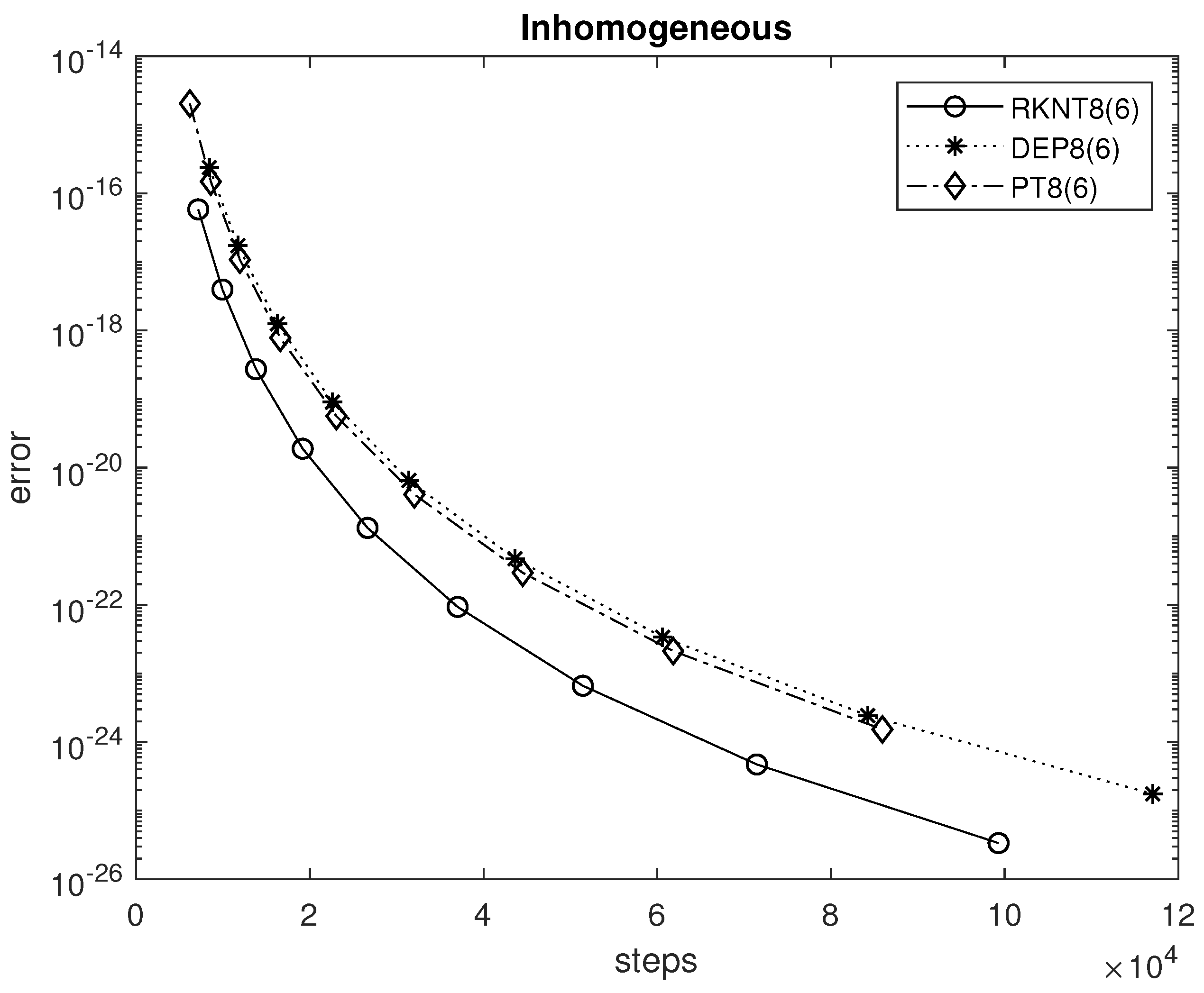
4.2.1. Inhomogeneous Equation
The inhomogeneous equation is the first test problem selected [21]:
with theoretical solution
We integrated this problem in the interval . In Figure 1, we draw the corresponding efficiency plots.

Figure 1.
Efficiency plots for the inhomogeneous equation.
4.2.2. Inhomogeneous Linear System
This problem is given as follows:
with theoretical solution
We integrated that problem in the interval and the efficiency plots are shown in Figure 2.
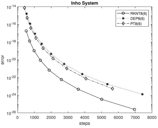
Figure 2.
Efficiency plots for the linear inhomogeneous system.
The rightmost circle in Figure 2 is justified by the following run of the Mathematica module given in the listing of the previous section.
In[1]:={solution, ireject} = RKNT86[{1/100*z1-1/10*z2,-1/10*z1+1/100*z2+Sin[x]},
{x,z1,z2}, {0,1,1},{-1000/10101,-(10100/10101)},10*Pi,10^-22];
In[2]={Length[solution] + ireject - 1, Max[Abs[Last[solution][[2 ;; 5]] -
{-1, -1, -1000/10101, -10100/10101}]]}
Out[2]={6957,2.419274*10^-26}
|
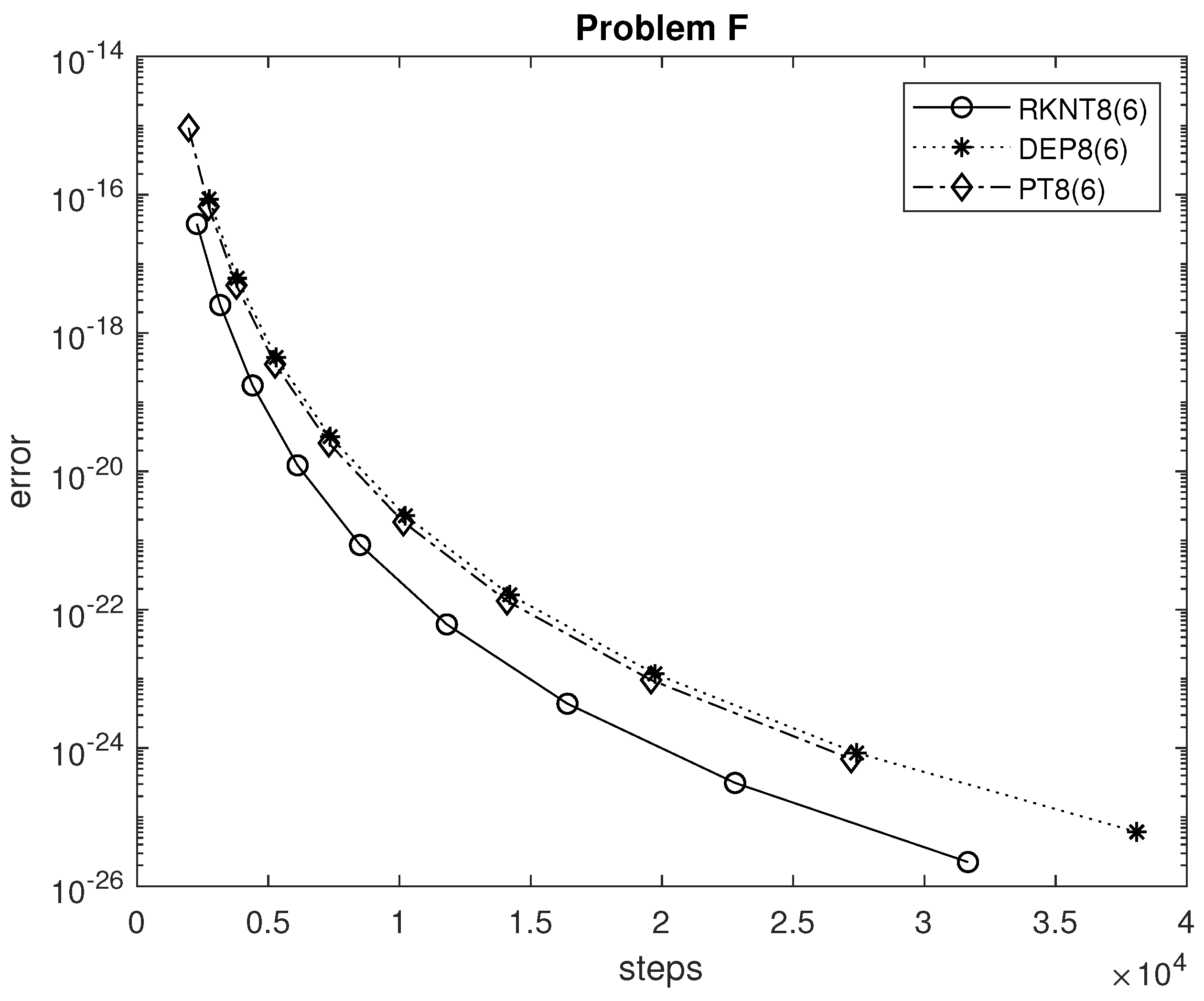
4.2.3. Problem F
Next we consider the following problem:
with initial values
and theoretical solution
Here, and may understood as components and not as time steps.
We integrated that problem in the interval . The theoretical solution and the efficiency plots are shown in Figure 3.
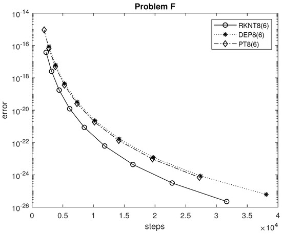
Figure 3.
Efficiency plots for problem F.
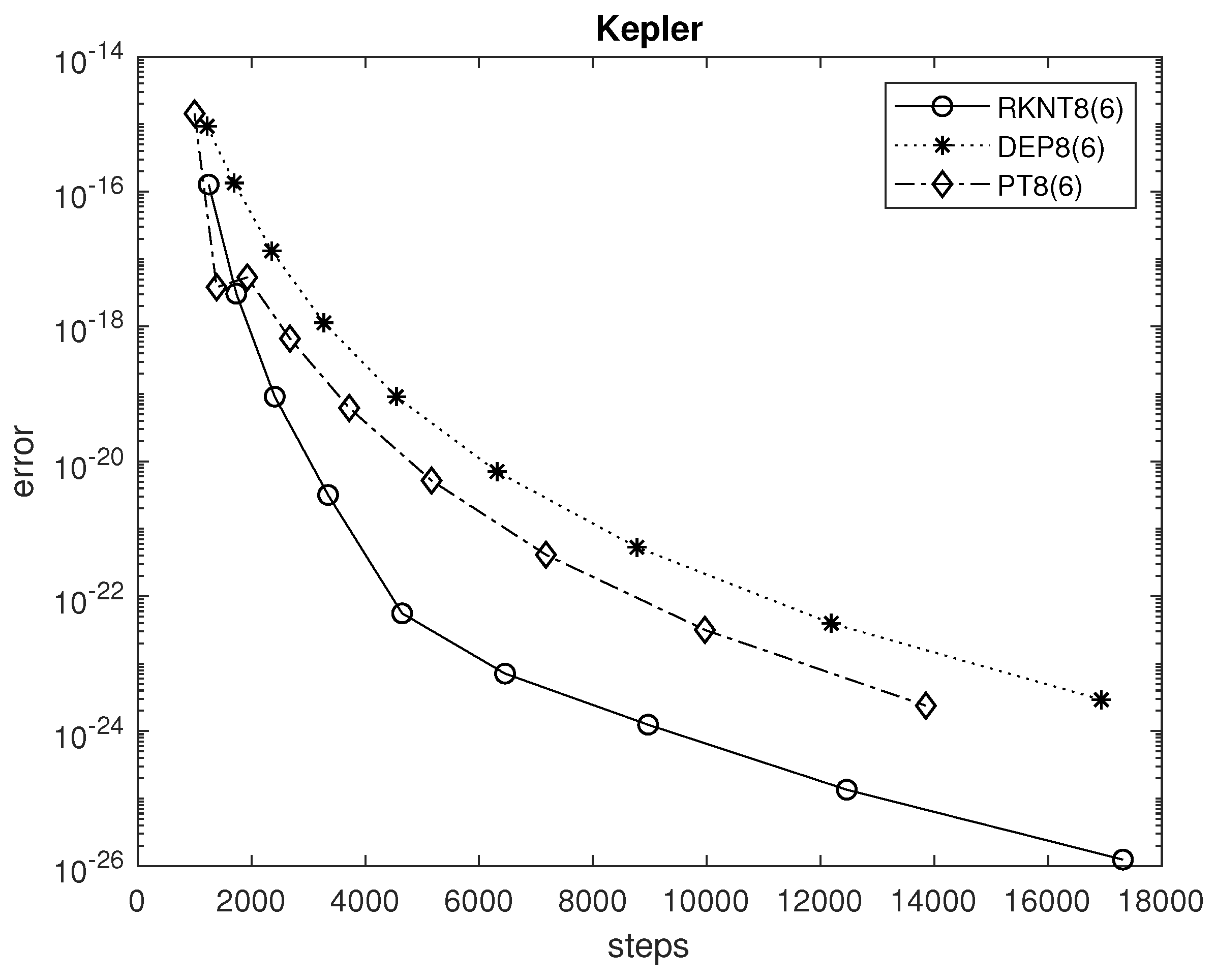
4.2.4. Kepler Problem
Next, we choose the celebrated two body problem with eccentricity ,
We solved the above equations in the interval as and the theoretical solution is given in [22]. The efficiency plots are shown in Figure 4.
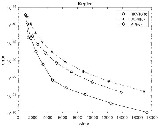
Figure 4.
Efficiency plots for the Kepler problem.
4.2.5. Coupled Non-Linear Pendulum
Finally, we considered a smooth variant of the non-linear problem from [2] pg. 297. The equations of motion are
We integrated the problem in the interval starting with no move or speed at all, i.e., .
No theoretical solution is available. Thus, the almost true solution is derived by running an integration using . The efficiency plots are shown in Figure 5.
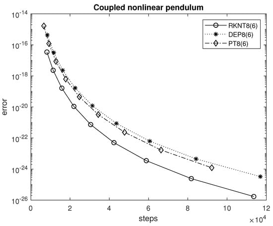
Figure 5.
Efficiency plots for the coupled non-linear pendulum.
4.3. Discussion on the Results
The results show that the new pair outperforms by far other RKN8(6) pairs on the problems tested. Almost 1–2 digits of accuracy were gained in most cases. The findings demonstrate that when high accuracies are required in the solution of special second order IVPs, the new approach significantly beats earlier ones.
5. Conclusions
In this paper, we looked at Runge–Kutta–Nyström pairs that are specifically optimized for solving initial value problems of second order when the first derivative is missing. We exploited the large coefficients that can be handled when working in quadruple precision arithmetic. The main contribution of our try is that the proposed method possesses very smaller truncation error terms in comparison with the other eighth order pairs appeared in the literature. Numerical tests in relevant problems justify our effort.
Reconsideration of other high order Runge–Kutta and Runge–Kutta–Nyström pairs may considered in the future in the direction shown here. Minimization of truncation errors for use in quadruple precision, regardless the increase in the magnitude of the coefficients.
Author Contributions
All authors have contributed equally. All authors have read and agreed to the published version of the manuscript.
Funding
The research was supported by a Mega Grant from the Government of the Russian Federation within the framework of the federal project No. 075-15-2021-584.
Institutional Review Board Statement
Not applicable.
Informed Consent Statement
Not applicable.
Data Availability Statement
The coefficients of the method can be retrieved in Mathematica format from http://users.uoa.gr/tsitourasc/rknt86.m (accessed on 4 February 2023).
Conflicts of Interest
The authors declare no conflict of interest.
References
- Hairer, E. Méthodes de Nyström pour l’équation différentielle y″ = f(x,y). Numer. Math. 1976, 2, 283–300. [Google Scholar] [CrossRef]
- Hairer, E.; Nørsett, S.P.; Wanner, G. Solving Ordinary Differential Equations I: Nonstiff Problems; Springer: Berlin/Heidelberg, Germany, 1993. [Google Scholar]
- Fehlberg, E. Eine Runge-Kutta-Nyström-Formel g-ter Ordnung rnit Schrittweitenkontrolle fur Differentialgleichungen . ZAMM 1981, 6, 477–485. [Google Scholar] [CrossRef]
- Dormand, J.R.; El-Mikkawy, M.E.A.; Prince, P.J. Families of Runge-Kutta-Nyström formulae. IMA J. Numer. Anal. 1987, 7, 235–250. [Google Scholar] [CrossRef]
- Dormand, J.R.; El-Mikkawy, M.E.A.; Prince, P.J. High-Order Runge-Kutta-Nyström formulae. IMA J. Numer. Anal. 1987, 7, 423–430. [Google Scholar] [CrossRef]
- El-Mikkawy, M.E.A.; Rahmo, E. A new optimized non-FSAL embedded RungeKuttaNyström algorithm of orders 6 and 4 in six stages. Appl. Math. Comput. 2003, 145, 33–43. [Google Scholar]
- Papakostas, S.N.; Tsitouras, C. High phase-lag order Runge–Kutta and Nyström pairs. SIAM J. Sci. Comput. 1999, 21, 747–763. [Google Scholar] [CrossRef]
- Simos, T.E.; Tsitouras, C. On high order Runge–Kutta– Nyström pairs. J. Comput. Appl. Maths. 2022, 400, 113753. [Google Scholar] [CrossRef]
- Jerbi, H.; Omri, M.; Kchaou, M.; Simos, T.E.; Tsitouras, C. Runge-Kutta-Nyström Pairs of Orders 8(6) with Coefficients Trained to Perform Best on Classical Orbits. Mathematics 2022, 10, 654. [Google Scholar] [CrossRef]
- Yoshida, H. Construction of higher order symplectic integrators. Phys. Lett. A 1990, 150, 262–268. [Google Scholar] [CrossRef]
- Calvo, M.P.; Sanz-Serna, J.M. High order symplectic Runge-Kutta-Nyström methods. SIAM J. Sci. Comput. 1993, 14, 1237–1252. [Google Scholar] [CrossRef]
- Brankin, R.W.; Gladwell, I.; Dormand, J.R.; Prince, P.J.; Seward, W.L. ALGORITHM 670: A Runge-Kutta-Nyström Code. ACM Trans. Math. Softw. 1989, 15, 31–40. [Google Scholar] [CrossRef]
- Butcher, J.C. On Runge-Kutta processes of high order. J. Austral. Math. Soc. 1964, 4, 179–194. [Google Scholar] [CrossRef]
- Kovalnogov, V.N.; Fedorov, R.V.; Karpukhina, M.T.; Kornilova, M.I.; Simos, T.E.; Tsitouras, C. Runge-Kutta-Nystrom methods of eighth order for addressing Linear Inhomogeneous problems. J. Comput. Appl. Maths. 2023, 419, 114778. [Google Scholar] [CrossRef]
- Tsitouras, C.; Famelis, I.T. Symbolic derivation of Runge-Kutta-Nyström order conditions. J. Math. Chem. 2009, 46, 896–912. [Google Scholar] [CrossRef]
- Price, K.V.; Storn, R.M.; Lampinen, J.A. Differential Evolution, A Practical Approach to Global Optimization; Springer: Berlin/Heidelberg, Germany, 2005. [Google Scholar]
- Storn, R.M.; Price, K.V. Differential evolution—A simple and efficient heuristic for global optimization over continuous spaces. J. Glob. Optim. 1997, 11, 341–359. [Google Scholar] [CrossRef]
- Storn, R.M.; Price, K.V.; Neumaier, A.; Zandt, J.V. DeMat. Available online: https://github.com/mikeagn/DeMatDEnrand (accessed on 18 August 2022).
- Matlab. MATLAB Version 7.10.0; The MathWorks Inc.: Natick, MA, USA, 2010. [Google Scholar]
- Wolfram Research, Inc. Mathematica, Version 11.3.0; Wolfram Research, Inc.: Champaign, IL, USA, 2018.
- Kovalnogov, V.N.; Kornilova, M.I.; Khakhalev, Y.A.; Generalov, D.A.; Simos, T.E.; Tsitouras, C. Fitted modifications of Runge–Kutta–Nyström pairs of orders 7(5) for addressing oscillatory problems. Math. Meth. Appl. Sci. 2023, 46, 273–282. [Google Scholar] [CrossRef]
- Enright, W.; Pryce, J.D. Two FORTRAN packages for assessing initial value methods. ACM Trans. Math. Softw. 1987, 13, 1–27. [Google Scholar] [CrossRef]


Disclaimer/Publisher’s Note: The statements, opinions and data contained in all publications are solely those of the individual author(s) and contributor(s) and not of MDPI and/or the editor(s). MDPI and/or the editor(s) disclaim responsibility for any injury to people or property resulting from any ideas, methods, instructions or products referred to in the content. |
© 2023 by the authors. Licensee MDPI, Basel, Switzerland. This article is an open access article distributed under the terms and conditions of the Creative Commons Attribution (CC BY) license (https://creativecommons.org/licenses/by/4.0/).