A Fast Forward and Inversion Strategy for Three-Dimensional Gravity Field

Abstract

Obtaining a three-dimensional (3D) density distribution within a reasonable time is one of the most critical problems in gravity exploration. In this paper, we present an efficient 3D forward modeling and inversion method for gravity data. In forward modeling, the 3D model is discretized into multiple horizontal layers, with the gravity field at a point on the surface being the sum of the gravity fields from all layers. To calculate the gravity field from each horizontal layer, we use the fast Fourier transform (FFT) method and the Block Toeplitz with Toeplitz Blocks (BTTB) matrix, which dramatically reduces both the computation time and storage requirement. In the inversion, the observed gravity data are separated into multiple gravity components of different depths using the cutting separation method. An iterative method is used to adjust the model to fit the above gravity component for each cutting radius. The initial model is constructed from the transformation of gravity components. These methods were applied to both synthetic data and field data. The numerical simulation validated the proposed methods, and the inversion results of field data were consistent with information obtained from well logging. The computational time and memory usage were also reasonable.

1. Introduction

Gravity surveying is an essential geophysical method, especially in large-scale exploration and local deposit exploration, which makes use of the density difference between ore and the host rock. Theoretically, by analyzing gravity data collected on the ground or in the air, we can infer underground geological conditions. However, the major difficulty of gravity data inversion is its inherent non-uniqueness. Any gravity field measured on the surface of the earth can be reproduced by infinitesimally thin density bodies beneath the surface. This means there is no accurate depth resolution inherent in a single gravitational field. However, if a plurality of gravity observation data can be evaluated, approximate depth resolution information can be drawn.

To obtain the density distribution of the underground medium from gravity data, previous researchers have developed and demonstrated a variety of different methods [1,2,3,4]. For gravity modeling and inversion, the 2D or 3D model domain needs to be discretized into a set of rectangular grids (2D) [5] or cuboid grids (3D) [6], each with a constant density. The number of elements is generally much greater than the number of datasets available, which is useful when solving an underdetermined problem. In order to meet certain accuracy requirements, the model is often separated into a very large number of elements. Therefore, it is necessary to find efficient algorithms to run the inversion [7,8]. For instance, to invert observed gravity data on a 100 × 100 grid, the model is divided into 30 layers. When the underground model is divided into 30 layers, and each layer into 100 × 100 units, there are 300,000 unknowns to solve. If we adopt a least-squares inversion method, the objective function can be transformed into a linear equation, and the size of its coefficient matrix will be $300,000\times 300,000$. It is difficult and costly to solve such a large-scale linear equation. In addition, the memory requirement of this coefficient matrix is extremely large (9 × 1010 data, with a memory requirement of approximately 335 GB).

Several algorithms have been developed to speed up inversion. For example, Yao et al. [9] proposed a stochastic subspace method, in which the geometric lattice frame was separated, calculated, and stored, which significantly sped up inversion. Wavelet-based methods [10] and footprint techniques [11] were introduced to speed up inversion by down-sampling a dense matrix to a sparse matrix. These methods can be applied in both the data and model domains [12,13].

The Fourier domain method was developed to produce variable density models, where first the analytical spectrum of a gravity field with certain variables is obtained, and then is transformed back into the space domain using fast Fourier transform (FFT) techniques. Subsequently, researchers studied the variable density models of gravity anomalies (e.g., linear or exponential prismatic models [14]) by using Fourier transform expressions [15,16]. Xu et al. [17] developed an inversion method using a potential field separation technique and downward continuation, where the gravity field is calculated by the frequency domain method. However, because there is no iterative fitting process, inversion precision cannot be guaranteed. Chen [18] implemented a fast and high-precision continuation method using the Block-Toeplitz Toeplitz-Block (BTTB) matrix and the FFT technique [19,20]. Since the BTTB matrix has symmetrical features, it is possible to compress storage on a large-scale. Zhang and Wong [21] developed an inversion method for large-scale gravity data using the BTTB matrix and a weighted regularized conjugate gradient inversion method. Both methods can greatly reduce memory consumption and increase computing speed in forward modeling due to the employment of the BTTB matrix and FFT techniques, but they use different methods to solve the problem of multiplying the vector by the matrix. Wu and Chen [22] proposed applying the Gauss-FFT method to gravity forward modeling, as the Gauss-FFT method is more accurate than the traditional FFT method. Cui [23] studied the magnetic fields simulation and data inversion of magnetic anomalies in the frequency domain.

In this paper, we propose a fast forward modeling and inversion scheme for gravity data. The cutting method and downward continuation are adopted to separate the observed gravity data, and the iterative inversion method is used to fit each gravity component. In this way, gravity data inversion avoids the solution process of large-scale linear equations, thus greatly improving efficiency.

2. Forward Modeling

The gravity field at a point on the ground can be calculated by [2]:

$$\Delta g=G{\displaystyle \underset{v}{\iiint }\frac{\sigma (\xi ,\eta ,\lambda )(\lambda -z)d\xi d\eta d\lambda }{{[{(\xi -x)}^2+{(\eta -y)}^2+{(\lambda -z)}^2]}^{3/2}}}$$

(1)

where $\left(x,y,z\right)$ is the observation location; $\left(\xi ,\eta ,\lambda \right)$ is the location of the anomalous body; and $\sigma (\xi ,\eta ,\lambda )$ is the density; G is the gravitational constant, $G=6.67\times {10}^{-11}{\mathrm{m}}^3/(\mathrm{kg}·\mathrm{m})$.

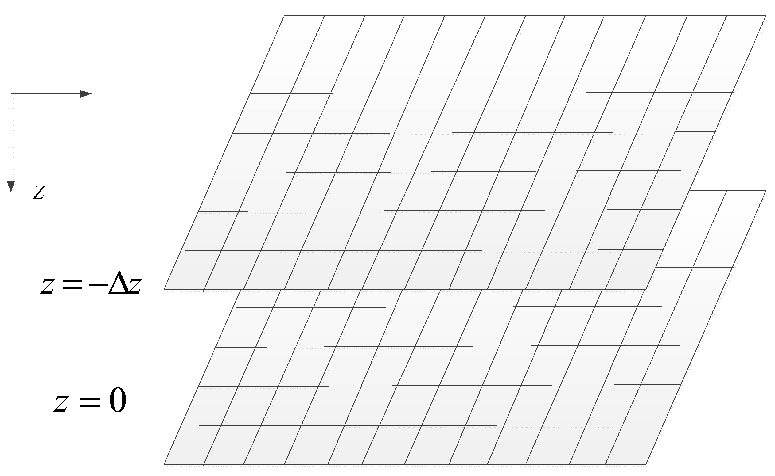
The field extension integral equation is:

$$f(x,y)=\frac{\Delta z}{2\pi }{\displaystyle \underset{s}{\iint }\frac{\Delta g(\xi ,\eta )}{{[{(x-\xi )}^2+{(y-\eta )}^2+\Delta z^2]}^{3/2}}d\xi d\eta }$$

(2)

where $\Delta g(\xi ,\eta )$ is the field at $z=0$, $f(x,y)$ is the field at $z=-\Delta z$.

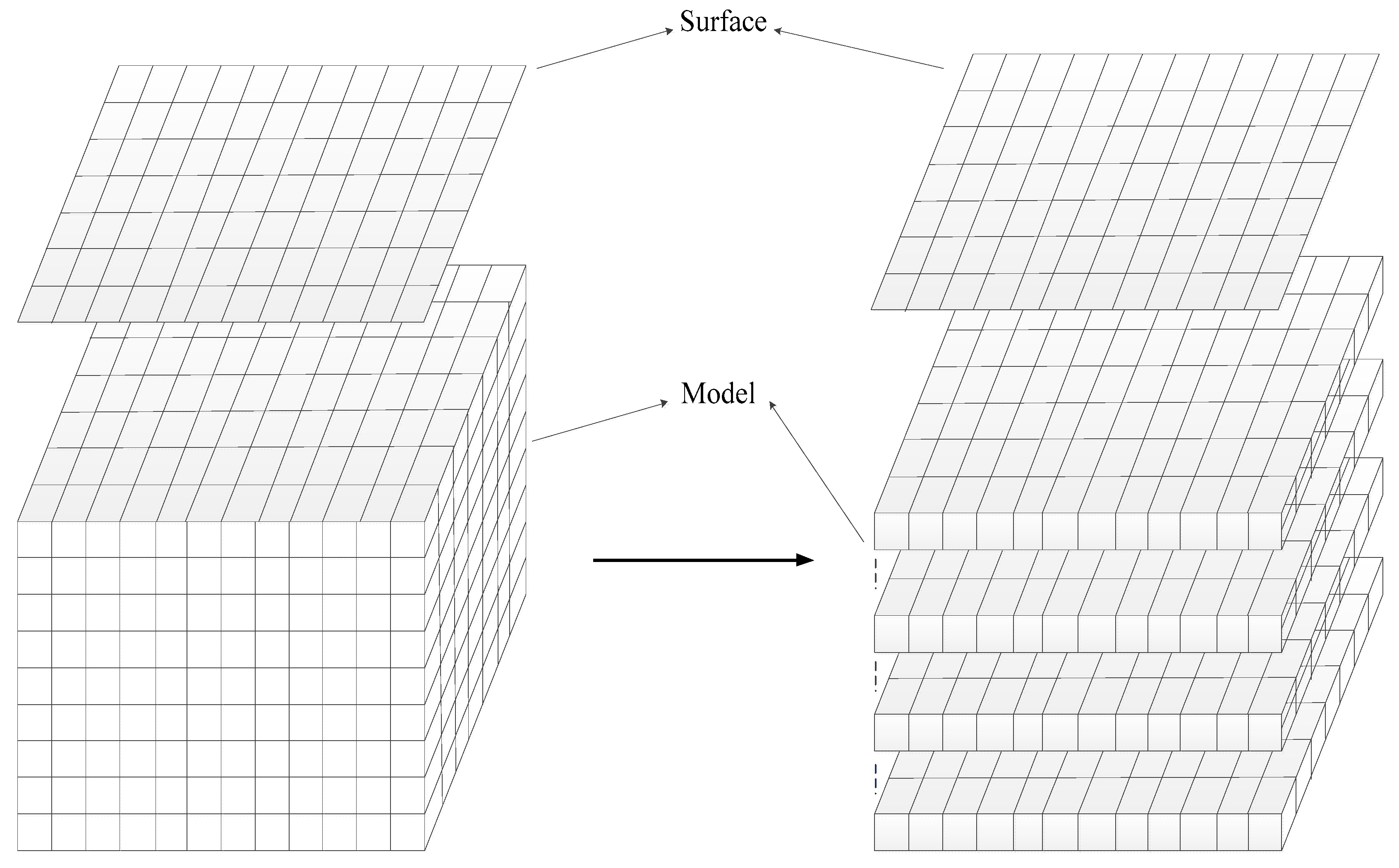
As one can see from the above, Equation (1) is a triple convolution equation and Equation (2) is a double convolution equation. The triple convolution equation can be treated as a superposition of the double convolution equation. In this way, we can translate the three-dimensional gravity forward problems into two-dimensional problems.

By comparing Figure 1 and Figure 2, we can see that the calculation of the gravity field of each layer is similar to gravity field upward continuation. We divide the model into several layers, use the new method to calculate the gravity field generated by each layer, and then compute the sum of these gravity fields. The sum is the total gravity field generated by the whole model.

Now let us take a brief look at the steps of our forward method. Firstly, we discretize the model. According to the mesh generation method, Equation (1) can be rewritten as follows:

$$\Delta g(x,y,z)\approx G{\displaystyle \sum _{k=1}^L{\displaystyle \sum _{j=1}^N{\displaystyle \sum _{i=1}^M\sigma (i,j,k)\frac{(\lambda -z)\Delta x\Delta y\Delta z}{{[{({\xi }_i-x)}^2+{({\eta }_j-y)}^2+{({\lambda }_k-z)}^2]}^{3/2}}}}}$$

(3)

where $(x,y,z)$ are the coordinates of the observation point, and $\left({\xi }_i,{\eta }_j,{\lambda }_k\right)$ are the coordinates of a cuboid cell with constant density.

The gravity field from a three-dimensional body contains M × N × L small rectangular units that can be treated as the superposition of L layers. with each layer containing M × N units. So, Equation (3) can be rewritten as follows:

$$\Delta g=G\Delta x\Delta y\Delta z{\displaystyle \sum _{k=1}^L(Z_k\cdot {\displaystyle \sum _{j=1}^N{\displaystyle \sum _{i=1}^M(\sigma (i,j,k)\frac{1}{{[{(i-m)}^2\Delta x^2+{(j-n)}^2\Delta y^2+Z_k{}^2]}^{3/2}})}})}$$

(4)

where $Z_k={\lambda }_k-z_k$. Let ${\xi }_i=i\cdot \Delta x,{\eta }_j=j\cdot \Delta y,{\lambda }_k=k\cdot \Delta z$, m, n are the numbers of the observation points along x and y directions, on the ground or in the air at a certain altitude, m = 1, 2, ⋯, M; n = 1, 2, ⋯, N. i, j, k are the order number of the cells along x, y and z directions. Here we emphasize again that using the traditional analytical calculation method to solve Equation (4) is very time-consuming, and new methods must be found to significantly improve computational efficiency.

Let:

$$Q={\displaystyle \sum _{j=0}^{N-1}{\displaystyle \sum _{i=0}^{M-1}(\sigma (i,j)\frac{1}{{[{(i-m)}^2\Delta x^2+{(j-n)}^2\Delta y^2+Z_k{}^2]}^{3/2}})}}$$

(5)

The equation can be further simplified into the following one:

$$Q=A(ii,jj){\sigma }_2$$

(6)

where:

$$A(ii,jj)=\frac{1}{{(R(m,n;i,j))}^3}$$

(7)

$$R(m,n;i,j)=\sqrt{{(i-m)}^2\Delta x^2+{(j-n)}^2\Delta y^2+Z_k{}^2}$$

(8)

$$ii=(m-1)\cdot N+n,ii=1,2,\cdots ,MN$$

(9)

$$jj=(i-1)\cdot N+j,jj=1,2,\cdots ,MN$$

(10)

${\sigma }_2 \mathrm{is} \mathrm{a} \mathrm{vector} \mathrm{converted} \mathrm{from} \mathrm{the} \mathrm{matrix} \sigma (i,j)$,

$${\sigma }_2=[\sigma (1,1),\sigma (1,2),\cdots ,\sigma (1,N),\sigma (2,1),\sigma (2,2),\cdots ,\sigma (2,N),\cdots ,\sigma (M,N-1),\sigma (M,N)]$$

(11)

A(ii,jj) is the coefficient matrix. In general, the dimensions of the A matrix are quite large, but it is in the same form as the BTTB matrix. The BTTB matrix has the following three characteristics: overall symmetry, block symmetry, and block matrix. All Toeplitz matrices can be written as follows:

$$A=\left[\begin{array}{ccccccc}{T}_0& T_{-1}& T_{-2}& \cdots & \cdots & T_{2-N}& T_{1-N}\\ T_1& T_0& T_{-1}& T_{-2}& \ddots & \ddots & T_{2-N}\\ T_2& T_1& T_0& \ddots & \ddots & \ddots & ⋮\\ ⋮& T_2& \ddots & \ddots & \ddots & T_{-2}& ⋮\\ ⋮& \ddots & \ddots & \ddots & T_0& T_{-1}& T_{-2}\\ T_{N-2}& \ddots & \ddots & T_2& T_1& T_0& T_{-1}\\ T_{N-1}& T_{N-2}& \cdots & \cdots & T_2& T_1& T_0\end{array}\right]$$

(12)

where each block T_j is a Toeplitz matrix, given by

$$T_j=\left[\begin{array}{ccccccc}{a}_{0,j}& a_{-1,j}& a_{-2,j}& \cdots & \cdots & a_{2-M,j}& a_{1-M,j}\\ a_{1,j}& a_{0,j}& a_{-1,j}& a_{-2,j}& \ddots & \ddots & a_{2-M,j}\\ a_{2,j}& a_{1,j}& a_{0,j}& \ddots & \ddots & \ddots & ⋮\\ ⋮& a_{2,j}& \ddots & \ddots & \ddots & a_{-2,j}& ⋮\\ ⋮& \ddots & \ddots & \ddots & a_{0,j}& a_{-1,j}& a_{-2,j}\\ a_{M-2,j}& \ddots & \ddots & a_{2,j}& a_{1,j}& a_{0,j}& a_{-1,j}\\ a_{M-1,j}& a_{M-2,j}& \cdots & \cdots & a_{2,j}& a_{1,j}& a_{0,j}\end{array}\right]$$

(13)

Therefore, Equation (4) can be expressed as the multiplication of A(ii,jj) (a BTTB matrix) and a vector. According to the symmetry of the BTTB matrix, we can use a vector t_j instead of the Toeplitz matrix T_j in computation.

$$t_j=(a_{M-1,j},a_{M-2,j},\cdots ,a_{1,j},a_{0,j},a_{1,j},\cdots ,a_{2-M,j},a_{1-M,j})$$

(14)

In this manner, Equation (14) can be replaced by the following:

$$A_1=\left[\begin{array}{ccccc}{a}_{1-M,1-N}& \cdots & a_{1-M,0}& \cdots & a_{1-M,N-1}\\ ⋮& ⋮& ⋮& ⋮& ⋮\\ a_{0,1-N}& \cdots & a_{0,0}& \cdots & a_{0,1-N}\\ ⋮& ⋮& ⋮& ⋮& ⋮\\ a_{M-1,1-N}& \cdots & a_{M-1,0}& \cdots & a_{M-1,N-1}\end{array}\right]$$

(15)

where $A\in C^{M^2\times N^2}$, and $A_1\in C^{(2M-1)\times (2N-1)}$. By padding $A_1$ with zeros, a matrix $A_1^{ext}$ with dimensions of $2M\times 2N$ can be obtained as

$$A_1^{ext}=\left[\begin{array}{cccccc}0& 0& \cdots & 0& \cdots & 0\\ 0& a_{1-M,1-N}& \cdots & a_{1-M,0}& \cdots & a_{1-M,N-1}\\ ⋮& ⋮& ⋮& ⋮& ⋮& ⋮\\ 0& a_{0,1-N}& \cdots & a_{0,0}& \cdots & a_{0,1-N}\\ ⋮& ⋮& ⋮& ⋮& ⋮& ⋮\\ 0& a_{M-1,1-N}& \cdots & a_{M-1,0}& \cdots & a_{M-1,N-1}\end{array}\right]$$

(16)

We divide the matrix $A_1^{ext}$ into 4 parts.

$$A_1^{ext}=\left[\begin{array}{cc}{a}_{11}& a_{12}\\ a_{21}& a_{22}\end{array}\right]$$

(17)

where $a_{11},a_{12},a_{21},a_{22}\in C^{M\times N}$.

By rearranging the 4 parts we obtain

$$B_1=\left[\begin{array}{cc}{a}_{22}& a_{21}\\ a_{12}& a_{11}\end{array}\right]$$

(18)

Next, we need to extend vector ${\sigma }_2$ to a matrix

$$D=\left[\begin{array}{cc}\sigma & 0_{M\times N}\\ 0_{M\times N}& 0_{M\times N}\end{array}\right]\in C^{2M\times 2N}$$

(19)

Now, matrix B₁ and matrix D are the same size, and we can use the FFT technique to find an efficient solution.

$${\tilde{B}}_1=fft2(B_1)$$

(20)

$$\tilde{D}=fft2(D)$$

(21)

$$\widetilde{Q^{\prime }}={\tilde{B}}_1.\ast \tilde{D}.$$

(22)

$$Q^{\prime }=ifft2(\widetilde{Q\prime }).$$

(23)

$$Q^{\prime }=\left[\begin{array}{cc}q{\prime }_{11}& q{\prime }_{12}\\ q{\prime }_{21}& q{\prime }_{22}\end{array}\right].$$

(24)

$$Q=q{\prime }_{11}.$$

(25)

where fft2 is the two-dimensional Fourier transform, and ifft2 is the two-dimensional inverse Fourier transform $q{\prime }_{11},q{\prime }_{12},q{\prime }_{21},q{\prime }_{22}\in C^{M\times N}$. Using the conventional method, Equation (1) can be rewritten as the convolution form (Equation (6)), but the calculation cost is very high. If it is converted from Equation (6) to Equation (21), the cost of a matrix–vector product in the frequency domain is reduced to O ((N × M) log (N × M)) which is much smaller than the original cost of O ((N × M)²). Therefore, Equation (21) can be computed very efficiently and accurately. Another improvement is that we use $A_1$ instead of A in the calculations and storage to further simplify the process. In contrast, Zhang and Wong [21] used matrix A to perform this calculation and their method was more complex, as explained further in the section ‘computational cost’.

To demonstrate the accuracy and efficiency of our forward modeling, we built a model with high-density and low-density anomalies (Figure 3a). The anomalous density of the low-density anomaly is −1 g/cm³. The model is a rectangular block, which extends from 1500 m to 2000 m along the x-axis, 1000 m to 2000 m along the y-axis, and 200 m to 400 m along the z-axis (vertical axis pointing downward). The anomalous density of the high-density anomaly is 1 g/cm³, which extends from 1000 m to 2000 m along the x-axis, 750 m to 2250 m along the y-axis, and 600 m to 800 m along the z-axis (Figure 3). We divide the whole model into 9 million (300 × 300 × 100) small cells with each cell having dimensions of 10 × 10 × 10 m³. Figure 3b shows the relative gravity field value calculated by our algorithm, Figure 3c shows a mathematical analytical solution, and Figure 3d shows the error distribution. We can see that the maximum error of the analytical solution is only 0.022%, which demonstrates the high accuracy of the proposed forward modeling method. Additionally, it only takes 6.5 s to compute such a large model (Performed on a desktop computer with Intel i5-4590 CPU, with 4 3.3 GHz cores).

3. Apparent Density Inversion

There are many ways to perform inversion on gravity datasets. We use an unconventional inversion strategy to avoid needing to solve many linear equations. Firstly, the observed gravity field is decomposed into multiple components with different cutting radiuses using the cutting separation method, where the cutting radius is equal to the depth of the layer. Then, an iterative method is used to adjust the model to fit the above gravity component for each cutting radius. Based on the relationship between the density and the gravity field, we then use an iterative method to invert the density of each layer. Finally, we obtain the density distribution by combining the results of each layer.

3.1. Gravity Field Separation

There are different kinds of methods to separate potential field data, including ones in both the spatial and frequency domains. They include the hand smooth method, extension method, moving average method, trend analysis method, cutting method, peeling method, filtering method, wavelet transform method. [24].

Cheng et al. [25] proposed a separation method, known as the cutting method, that uses a cutting operator to separate the observed gravity anomalies many times until the surface of gravity is cut to a certain degree of smoothness. Tests showed that this method was not limited by the area of calculation, it did not produce artificial anomalies, and it had a fast calculation speed. Subsequent researchers have improved the cutting separation method significantly [26,27].

In this paper, we use the average value method with an 8-point window (Figure 4) to separate gravity fields into different layers. Experiments showed that the 8-point window method is better than the 4-point window method [24], as the 8-point window method effectively reduced the error in the iterative separation process and improved the accuracy of gravity field separation. Its basic principle is described as follows:

Calculate the average gravity field of 8 points around the target point

$$\begin{array}{ll}A(x,y)=& \frac{1}{8}[\Delta g(x-r,y-r)+\Delta g(x+r,y-r)+\Delta g(x-r,y+r)+\Delta g(x+r,\\ & y+r)+\Delta g(x-r,y)+\Delta g(x+r,y)+\Delta g(x,y-r)+\Delta g(x,y+r)]\end{array}$$

(26)

where $r$ is the cutting radius of gravity field separation. Based on many models and practical data tests, the thickness of the target layer is approximately equal to $r$.

• Calculate the gravity field without the target layer

$${\Delta g(x,y)}^{\prime }=a\Delta g(x,y)+bA(x,y)$$

(27)

with

$$a=\frac{1}{4}(\frac{{(\Delta B_x)}^2}{{(\overline{\Delta B_x})}^2+{(\Delta B_x)}^2}+\frac{{(\Delta B_y)}^2}{{(\overline{\Delta B_y})}^2+{(\Delta B_y)}^2}+\frac{{(\Delta B_{xy})}^2}{{(\overline{\Delta B_{xy}})}^2+{(\Delta B_{xy})}^2}+\frac{{(\Delta B_{yx})}^2}{{(\overline{\Delta B_{yx}})}^2+{(\Delta B_{yx})}^2})$$

(28)

$$b=1-a$$

(29)

$$\{\begin{array}{l}\Delta B_x=\Delta g(x+r,y)-\Delta g(x-r,y)\\ \Delta B_y=\Delta g(x,y+r)-\Delta g(x,y-r)\\ \Delta B_{xy}=\Delta g(x+r,y+r)-\Delta g(x-r,y-r)\\ \Delta B_{yx}=\Delta g(x-r,y+r)-\Delta g(x+r,y-r)\\ \overline{\Delta B_x}=\Delta g(x,y)-\frac{1}{2}[\Delta g(x+r,y)+\Delta g(x-r,y)]\\ \overline{\Delta B_y}=\Delta g(x,y)-\frac{1}{2}[\Delta g(x,y+r)+\Delta g(x,y-r)]\\ \overline{\Delta B_{xy}}=\Delta g(x,y)-\frac{1}{2}[\Delta g(x+r,y+r)+\Delta g(x-r,y-r)]\\ \overline{\Delta B_{yx}}=\Delta g(x,y)-\frac{1}{2}[\Delta g(x-r,y+r)+\Delta g(x+r,y-r)]\end{array}$$

(30)

2.

Calculate the gravity field of the target layer

$${\Delta g(x,y)}^{″}=\Delta g(x,y)-\Delta g{(x,y)}^{\prime }.$$

(31)

$\Delta g{(x,y)}^{″}$ is the gravity field of the target layer with a thickness of $r$. $\Delta g{(x,y)}^{\prime }$ is the gravity field of the model without the target layer, also termed the residual field. By using the average value method, we can obtain the gravity field of the layers of the model in different depths.

In order to demonstrate the effectiveness of the 8-point window method, we built a 4-layer model. The thickness of each layer is 150 m. There are five anomalous bodies in the first layer; the corresponding relative densities are: 0.5 g/${\mathrm{cm}}^3$, 0.9 g/${\mathrm{cm}}^3$, −1 g/${\mathrm{cm}}^3$, 1 g/${\mathrm{cm}}^3$, 0.8 g/${\mathrm{cm}}^3$. There are two anomalous bodies in the second layer; the corresponding relative densities are: 1.8 g/${\mathrm{cm}}^3$ and 1.5 g/${\mathrm{cm}}^3$. There are two anomalous bodies in the third layer with anomalous densities of 1.5 g/${\mathrm{cm}}^3$ and 1.8 g/${\mathrm{cm}}^3$. In the last layer, there are also two anomalous bodies with anomalous densities of 0.5 g/${\mathrm{cm}}^3$ and 1.2 g/${\mathrm{cm}}^3$. The gravity field of each layer is calculated and summed up to a total field of the whole model (Figure 5b).

We assume the total fields are composed of 4 layers, where each layer has a thickness of 150 m and the cutting radiuses are 150 m, 300 m, 450 m, and 600 m. By using the 8-point average method, the total field is separated into gravity fields of 4 layers; layers 1–4 are shown in Figure 5c. We can see that the separated gravity fields are very similar to the gravity field of each layer (Figure 5b). The sum of separated gravity fields (Figure 5c) is similar to the gravity field of the whole model (Figure 5b) as well. Generally, the more layers that are used in field separation, the less residual gravity fields that are produced, and the better the separation results will be.

3.2. Inversion Algorithm

In the early 1990s, researchers began to work on layer apparent density inversion. Mu et al. [28] proposed a method to calculate the apparent density of the formation based on the gravity anomaly caused by a certain stratum. This method divides the formation into m × n cells with a size of Δx × Δy × Δz. The gravitational field generated by the formation is the superposition of the gravitational field generated by m×n small cells. To finish the apparent density inversion, the gravity field is transformed to the frequency domain using an FFT, and then the frequency spectrum is used to calculate the approximate distribution of the formation density. The advantage of this method is that the processing speed is faster. However, the inversion is unstable at high frequencies. To solve this unstable inversion problem, Xu et al. [29] extended the gravity field to the top surface of the formation, which improved the stability of the inversion. However, studies indicate that potential field downward continuation is an ill-conditioned problem. The potential field cutting and separation process can produce small unwanted anomalies in the data. Downward continuation can amplify the anomalies, which results in false anomalies.

Here, we propose an iterative inversion method. Theoretically, the starting model is an arbitrary model. In order to speed up the convergence, however, we convert the measured gravity data into an initial model. We then calculate the differences between the modeled data and the measured data, which are then used to derive a model update.

$$m_0=\Delta g_0/\Delta g_{\max }\cdot {\sigma }_{pre}$$

(32)

where $\Delta g_0$ is the observed gravity data; $\Delta g_{max}$ is the maximum value of $\Delta g_0$; and ${\sigma }_{pre}$ is the density of background rock.

In potential field continuation, the methods most often used are the equivalent source method and fast Fourier transform (FFT). The equivalent source method requires solving extensive linear algebraic equations, and its calculation time is long. FFT is only applicable to the upward continuation of the plane potential field, and the downward continuation is very unstable. The iterative method discussed in this paper does not need to solve algebraic equations, and it is suitable for the upward and downward continuation of the surface potential field. Additionally, it has good stability, high calculation speed, and accuracy.

We calculate the modeled data using the starting model based on the following equation:

$$\Delta g_i=F(m_{i-1})$$

(33)

where $i=1,2,3\cdot \cdot \cdot n$, $n$ is the total number of iterations, and $F$ stands for forward program.

The model update $\Delta m$ is derived by

$$\Delta m=\alpha \cdot (\Delta g_0-\Delta g_i)/\Delta g_{\max }\cdot {\sigma }_{pre}.$$

(34)

where $\alpha$ is the convergence coefficient. If $\alpha$ is too large, the inversion process will fluctuate. Otherwise, the convergence will be too slow. After several model tests, when $\alpha$ is equal to 0.5, the iterative convergence is fast and stable (Figure 6). However, we recommend selecting a suitable convergence coefficient in the range of 0~1.0 when conducting field data inversion. Since the model modification Δm is the product of the ratio of the gravity difference to the maximum gravity value (0~1.0) and the relative density of the rock, the usual variation range of the adjustment coefficient α should be consistent with normalized gravity, that is, between 0 and 1.

With the model update, the revised model is

$$m_i=m_{i-1}+\Delta m.$$

(35)

Then we go back to Equation (33) for the next iteration. The inversion will stop when the difference is less than a pre-set threshold. Usually, we can obtain a satisfactory inversion result after about 50 iterations.

3.3. Synthetic Studies

Two synthetic models were built to demonstrate the efficacy of the inversion algorithm. The first synthetic model has two anomalies (500 m × 1000 m × 200 m), which have a relative high density of 0.5 g/${\mathrm{cm}}^3$ (left) and a relative low density of −1 g/${\mathrm{cm}}^3$ (right) respectively, and they are 1000 m apart (Figure 7a). The forward modeled gravity field is shown in Figure 7b. We invert the data and plot the vertical slice at y = 1500 m (Figure 7c) and the horizontal slice at z = 600 m (Figure 7d). The horizontal positions and extents of the anomalies are very well reconstructed, but the depths of the inverted model are shallower than the true model. The inverted densities are less than the densities of the true model, with a maximum of 0.1 g/${\mathrm{cm}}^3$ and a minimum of −0.2 g/${\mathrm{cm}}^3$, which are about 20% of those in the true model. In addition, the left and right boundaries show a tendency to outward expansion, but there is no such phenomenon at the boundaries in y direction (Figure 7d). These are artifacts due to the boundary effects.

The second synthetic model is a dyke model, which simulates inclined ore bodies with higher density. As shown in Figure 8b, the relative density of the dyke is 1 g/${\mathrm{cm}}^3$, which is composed of 6 one-hundred-meter-thick rectangular bodies. It extends from −100 m to −700 m along the z-axis, from 750 m to 2700 m along the x-axis, and from 1000 m to 2000 m along the y-axis. There is a density anomaly body in the upper left of the step model and its relative density is 1 g/${\mathrm{cm}}^3$. It extends from −200 m to −300 m along the z-axis, from 750 m to 1250 m along the x-axis, and from 1000 m to 2000 m along the y-axis. Figure 8a shows the forward modeled gravity field.

Figure 8c shows the slice of the inversion result at y = 1500 m. The inversion results are consistent with the true model (black outline in Figure 8c); however, two anomalies could not be clearly separated. The inclination of the ladder model is deviated by the upper left anomaly. Figure 8d shows the three-dimensional inversion relative density horizontal slice map.

These two synthetic models demonstrate that the proposed inversion algorithm can provide reliable inversion results. The resolution of the inversion results in the horizontal direction is relatively accurate, but the resolution in the depth direction is lower than that in the horizontal direction, which is a common problem with inversion. Additionally, the resolution of overlapping anomalies needs to be improved.

3.4. Case Study

Figure 9 shows the observed gravity field of one area in XinJiang, China. There was a higher gravity anomaly at the center of the survey area, which showed a ribbon shape along the east–west direction. Mineral deposits containing nickel were found in this area. The host rocks were mafic and ultramafic rocks, and the density of nickel ore was relatively high.

To test the proposed method, the inversion of real datasets was required. Firstly, we built a model with 24 layers that had 794 × 693 cells in each layer. Then, we separated the gravity field using the 8-point average method to carry out the gravity data inversion. The inversion results are shown in Figure 10, which indicated a weak high-density anomaly (about 0.15 g/${\mathrm{cm}}^3$) at the position of the high gravity field in the slice at z = −200 m. Moving down to z = −400 m, the density value was higher. The maximum density value was about 0.43 g/${\mathrm{cm}}^3$. At the depth of z = −800 m, there was no obvious density anomaly. We plotted the vertical slice at x = 1500 m, which clearly illustrated the density distribution over depth (Figure 11). Compared with the density data from well logging, the high-density anomaly in the inversion results was at approximately the same depth as the high density obtained from borehole data, which demonstrated the effectiveness of the inversion method.

4. Discussion of Computational Cost

In potential field continuation, the most common methods are the equivalent source and FFT methods. The equivalent source method requires solving extensive linear algebraic equations with a high computational cost, and FFT is only applicable to the upward continuation of the plane potential field since the downward continuation is very unstable. The iterative method in this paper does not solve algebraic equations and is suitable for the upward and downward continuation of the surface potential field. Additionally, it is stable, has low computational cost, and provides accurate results.

Regarding the iterative convergence problem, Equation (34) satisfies the first theorem of convergence, where it is a continuous first-order derivative at the right end of Equation (34) in the interval [0, σ_pre]. When Δm ∈ [0, σ_pre], there is 0 < |d(α∙(∆g₀ − ∆g_i)/∆g_max∙σ_pre)/d(Δm)| < 1. Therefore, Equation (34) converges if it satisfies the condition but does not satisfy the condition Just diverge. The iteration factor α is to balance the influence of σ_pre > 1. When σ_pre > 1, α can take the reciprocal of σ_pre. When α is 0, the iteration cannot be performed. When α is small, the convergence is slower but stable. When α is larger, the convergence is faster, but the iterative process will oscillate.

We discuss computational costs in this section due to their importance for economy. The computations in this paper were performed on a desktop with Intel i5-4590 CPU (4 cores, 3.3 GHz) and 8 GB memory, which was shown in

Table 1. Computational cost for forward modeling and inversion.

	Number of Unknowns	Number of Iterations	Time (Second)
Forward	9 million (300 × 300 × 100)	1	6.20
Inversion (Synthetic models)	0.9 million (300 × 300 × 10)	50	85.70
Inversion (Field data)	13.2 million (794 × 693 × 24)	50	1661.50

. In the forward modeling example, it took about 6.2 s to calculate the 9 million (300 × 300 × 100) units, and the error from the theoretical value was only in the order of magnitude of 10⁻⁵. In the inversion, the model was divided into 10 layers. It took about 85.7 s for the 900,000 (300 × 300 × 10) units to rebuild the density distribution. In the case study, there were about 13.2 million units to calculate, which is a huge workload. However, it only took approximately 1661.5 s for our algorithm to run the inversion.

Zhang and Wong [21] studied a similar forward algorithm. Their computation was performed on a laptop with i7-3632QM CPU and 12G RAM. According to CPU performance ranking, the performance of the i5-4590 CPU and i7-3632QM CPU is approximately equal. Their calculation took 186.82 s to finish the inversion with 300,000 unknowns while our calculation took 85.7 s to finish the inversion of 900,000 unknowns. This shows that our proposed method was much more efficient, with a greatly reduced running time. Therefore, we believe that our newly developed method is fast enough and suitable for large-scale gravity field simulation and gravity dataset inversion.

5. Conclusions

In this paper we proposed an efficient 3D gravity forward modeling and inversion method which is fast, accurate, and requires reduced physical memory, and applied it to invert gravity datasets. The proposed method did not solve linear equations in the process of inversion. We transformed complex three-dimensional problems into relatively simple two-dimensional forward modeling problems. The gravity field separation method and the layered iterative inversion method were applied to achieve fast inversion. By combining our forward and inversion methods, the inversion speed can be accelerated and memory consumption can be greatly reduced. The tests on both synthetic models and field data show that this method is a robust and efficient method that produces reliable inversion results. This inversion method is suitable for large-scale inversion of practical gravity data.