Abstract
The paper concentrates on the solitary waves that are retrievable from the generalized Boussinesq equation. The numerical simulations are displayed in the paper that gives a visual perspective to the model studied in neurosciences. The Laplace–Adomian decomposition scheme makes this visualization of the solitons possible. The numerical simulations are being reported for the first time using an elegant approach. The results would be helpful for neuroscientists and clinical studies in Medicine. The novelty lies in the modeling that is successfully conducted with an impressively small error measure. In the past, the model was integrated analytically only to recover soliton solutions and its conserved quantities.
Keywords:
mathematical biology; generalized Boussinesq equation; solitons; neuroscience; Adomian-Laplace decomposition scheme MSC:
35Q92; 35C08
1. Introduction
The dynamics of solitons in biomembranes is modeled by the Hodgkin–Huxley equation (HHE) that was based on a dissipative process and is consequently not isentropic. Their discovery led to being recipients of Nobel Prize in Medicine during 1963. This model, namely the HHE, did not consider many crucial issues. Its structure is based on the equilibration of ion gradients across the nerve membrane through specific ion-conducting proteins (referred to as ion channels) which leads to transient voltage changes. HHE relies on the dissipative processes and is not isentropic. It is rather based on Kirchhoff circuits involving capacitors (nerve membranes), resistors (ion channels) and electrical currents introduced by the ion fluxes [1].
During 2011, an appropriate model was proposed that is based on the Boussinesq equation (BE) [1]. Many of the discrepancies with the HHE were overcome with the proposed BE as the governing model. The reversible temperature and heat changes that were observed in the context of the nerve pulse suggested that an isentropic process is responsible for the action potential. Next, the proposed BE naturally predicts the correct pulse propagation velocities in myelinated nerves as these are closely related to the lateral sound velocities in the nerve membrane. Additionally, BE does not explicitly contain ion channel proteins but assumes their effects are being embodied in empirically known macroscopic thermodynamic observations. Finally, the thermodynamic nature of the soliton model permits a simple and quantitative description of the action of anesthetics and its dependence on changes in intensive variables, such as hydrostatic pressure, as with their familiar effects on the phase transition temperature. These arguments gave way to the viable model, BE, which was proposed during 2011 [1].
BE was later studied analytically using the method of undetermined coefficients to locate the solitary waves that gave the model for the neurons propagating through the nerve cells [2]. The conservation laws were also identified in the same model. The conserved densities as well as the conserved quantities were enumerated. The parameter constraints that naturally emerged from these analyses were also enumerated [2].
The current paper studies these solitary waves, modeling the neurons, from a numerical perspective. The Laplace–Adomian decomposition method (LADM) was adopted to address the governing model numerically. The surface plots of such neurons were recovered with the LADM and the error measures were also tabulated and plotted. This error measure is of the order of , which is an impressively low count. The results are enumerated in the rest of the paper after a succinct review of the model and a brief introduction to the LADM.
2. Soliton Solution and Governing Equation
Here, we consider the propagation of solitons in biomembranes, which are essential components of nerve axons and all other varieties of living cells [3].
The dynamical behavior of solitons in biomembranes is governed by the generalized BE, provided by:
is the change in membrane area density as a function of x and t, where the nerve axon is modeled as a one-dimensional cylinder with lateral density excitations propagating along the coordinate x and time t. In addition, because an actual nerve is not isolated but is viscously coupled to the surrounding fluids, the parameters and represent the biomembrane’s nonlinear elastic behavior, whereas and are experimentally determined parameters determining the density dependence of sound velocity. Finally, and c are parameters that measure the friction and dispersion of the nerve axon, respectively.
The model described above was formally derived in [4] under two assumptions: (a) that membranes are at temperatures somewhat higher than their melting transition and (b) that the system is quasi one-dimensional, that is, the model predominantly applies to myelinated nerves, which are more resistant to curvature variations.
To retrieve for the 1-soliton solution to this model, the following ansatz [1,2] is considered
where the amplitude A is described by using the model parameters as follows:
the inverse width B is given using the model coefficients by
and
These relationships demand directly the constraint conditions
and
In addition, the following relations between the coefficients in Equation (1) must be satisfied for solitons to exist:
The mathematical model (1) has been used in several neuroscience-related investigations; for additional references, see [5,6,7,8,9] and references therein.
3. A Brief Exposition of Laplace–Adomian Decomposition Method (LADM)
G. Adomian and R. Rach developed the Laplace–Adomian decomposition method (LADM) to solve a wide class of nonlinear differential equations in [10] in 1986. Since 1986, LADM has been one of the most effective mathematical techniques for generating accurate numerical approximation solutions for a variety of nonlinear problems, arising from Physics, Chemistry, Biology, Finance or Engineering. A principal advantage of LADM is that it may be immediately used to any forms of differential equations, either linear or nonlinear, ordinary or partial, homogeneous or inhomogeneous, with constant or variable coefficients. Importantly, the LADM does not need linearization, discretization, or perturbed parameters in order to solve nonlinear problems [11]. However, the LADM has certain disadvantages, since we know that this approach provides an approximate solution of the problem by means of a series of functions. The region and rate of convergence of the series solution could be the problem. As the resulting series may be fast convergent in a very small region, but has a slow convergence rate in larger regions, the approximated series is an unacceptable solution in this region, hence limiting the area of application of the method [12].
In this section, the Adomian decomposition approach coupled with the Laplace transform will be shown briefly. The reader interested in further information about this methodology may look at [13].
To explain the fundamental principle behind the Laplace–Adomian decomposition procedure, we will take into account the operational formulation of the nonlinear partial differential equation of the second order:
with the conditions of position and rate of change at time given by
where F represents a differential operator. The operator F may be subdivided into , where L acts on q as . R and N are brief notations for the linear and nonlinear components, respectively, that are still present. In light of these considerations, Equation (10) may be rewritten as
Solving for and implementing the Laplace transform with respect to t to Equation (12), we obtain the following result:
In the following, we will refer to the action of on as . Moreover, taking into account the well-known property of the Laplace transform for the second derivative with respect to t:
When all of this is taken into consideration, Equation (13) becomes equal to
In view of the initial conditions provided by Equation (11), we have
By applying the inverse Laplace transformation to both sides of Equation (16), we are able to obtain
The procedure for Laplace–Adomian decomposition presupposes that the solution may be extended into a series provided by
In addition, the action of the nonlinear operator is represented as follows:
Each is an Adomian polynomial that can be determined for all varieties of nonlinearity using the expression below [14]:
The derivation of the formula (20) and the convergence of the series (19) can be found at the end of the manuscript in Appendix A.
Therefore, Adomian’s polynomials are given by
Similarly, the other polynomials are computed.
Consequently, Equation (21) provides the subsequent iterative algorithm:
Clearly, the relation (22) transformed the considered differential equation into an impressive determination of computable components.
Finally, after determining ’s, the N-term truncated approximation of the solution is obtained as
The Adomian decomposition technique coupled with the Laplace transform needs less work than the classic Adomian decomposition approach, as shown by this analysis. This technique rapidly reduces the amount of computations. Moreover, the Adomian decomposition process may be created without linearizing the equation.
4. Solution of the Generalized BE (1) by LADM
In this section, we outline the application of LADM to obtain soliton-type solutions for Equation (1) with the initial conditions
Let us consider the generalized BE (1) in an operator form
When the nonlinear operator N is subdivided into four components, as shown below, we get:
In addition, is the linear part of the operator and L is the second order operator given by .
In our case, the nonlinear terms , , and can be written as a series having Adomian polynomials as terms:
and
The Adomian polynomials , , and will be calculated using the Formula (20). The first few Adomian polynomials are given by
⋮
⋮
⋮
⋮
The Adomian polynomials , corresponding to the nonlinear part , are then given by
⋮
and so on for other Adomian polynomials.
Finally, the M-approximate solution for Equation (1) via LADM is given by
where each component is generated using algorithm:
Using software such as Mathematica, Matlab, etc., the solution to an M-term approximation provided by Equation (30) may be utilized easily for numerical simulations.
Since LADM is not a point approximator based on discretizations, its findings converge more quickly and are more accurate than those of the standard Adomian approach and numerical techniques, hence constituting a significant advance. This numerical approach demonstrates how the Laplace transform may be used to simulate the solutions of nonlinear partial differential equations by reconfiguring the decomposition method.
For more details of the method, as well as for specific applications to solitary waves, see [15]. For further information on the convergence of the suggested approach, see [16,17].
In [18], the authors demonstrate how they used the same methodology to a different biomathematics research problem, providing more evidence of the reliability of our methodology.
In the next section, we will demonstrate the usefulness of the LADM-derived algorithm by demonstrating its performance with four different cases.
5. Numerical Simulations and Graphical Results Presentation
Using the technique from the previous section, we will simulate the behavior of the produced solitons on biomembranes. This will include consideration of the hypothetical parameters listed in Table 1.

Table 1.
Parameters used for simulating solitons.
Figure 1, Figure 2, Figure 3 and Figure 4 depict the outputs of simulations conducted on the cases listed in Table 1. Additionally, in each case, the maximum error produced by LADM is graphically shown and compared to the maximum error produced by the Adomian standard method. All simulations were conducted using the Mathematica 13.2 software.
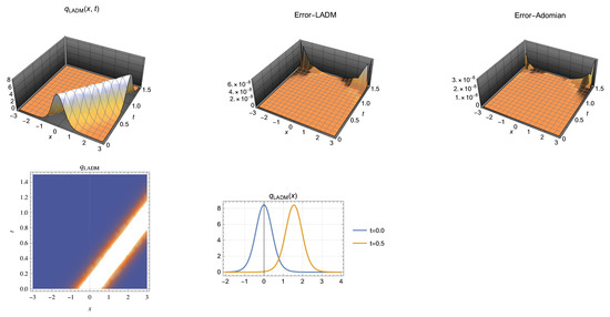
Figure 1.
Soliton profile in the interval , for the parameters selected in Case 1 (above left). Error by LADM (above center) and error by Adomian method (above right)). Density graph (bottom left). Two dimensional (2D) graph for and (bottom right).
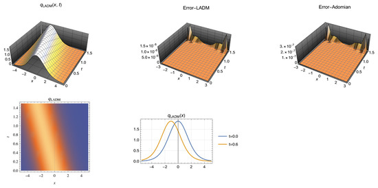
Figure 2.
Soliton profile in the interval , for the parameters selected in Case 2 (above left). Error by LADM (above center) and error by Adomian method (above right)). Density graph (bottom left). Two dimensional (2D) graph for and (bottom right).
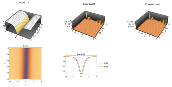
Figure 3.
Soliton profile in the interval , for the parameters selected in Case 3 (above left). Error by LADM (above center) and error by Adomian method (above right)). Density graph (bottom left). Two dimensional (2D) graph for and (bottom right).
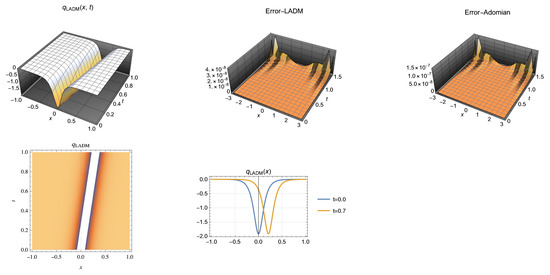
Figure 4.
Soliton profile in the interval , for the parameters selected in Case 4 (above left). Error by LADM (above center) and error by Adomian method (above right)). Density graph (bottom left). Two dimensional (2D) graph for and (bottom right).
6. Observations on Results and Figures
From Figure 1 and Figure 2, we can see that the solutions of Equation (1) have a restricted maximum amplitude and a minimum propagation velocity that is comparable to the pulse velocity in myelinated neurons. Under initial conditions, there are periodic solutions that exhibit neuronal excitability and latency periods. These results correspond with those previously found by researchers and presented in [19].
7. Conclusions
In this paper, LADM was used for the first time to retrieve the solitary waves, or neurons, for the generalized Boussinesq equation that numerically described the flow of neurons via nerve cells. The error measures are tabulated as well as plotted, thus expositing the fact that LADM is indeed a very powerful scheme to numerically analyze the higher order Boussunesq equation for neurosciences where the model is applicable.
In the future, the model will be addressed by additional numerical schemes and these include the variational iteration method, the finite element method and several others. The results would be available and disseminated across the board in a variety of journals.
Author Contributions
Writing—original draft preparation, Visualization, O.G.-G.; Conceptualization, Supervision, A.B.; Investigation, Software, L.M.; Supervision, A.A.A. All authors have read and agreed to the published version of the manuscript.
Funding
This research received no external funding.
Institutional Review Board Statement
Not applicable.
Informed Consent Statement
Not applicable.
Data Availability Statement
Not applicable.
Acknowledgments
This work was supported by the project “DINAMIC”, Contract no. 12PFE/2021.162. The authors are extremely thankful for it.
Conflicts of Interest
The authors declare no conflict of interest.
Appendix A. Adomian Polynomial Formula
In this appendix we will deduce Equation (20) that explains for every term in the sequence of the Adomian polynomials accepting the following assumptions stated in [22]:
- (a)
- The series solution, , of the problem given in Equation (18) is absolutely convergent,
- (b)
- The nonlinear function can be expressed by means of a power series whose radio of convergence is infinite, that iswhere, .
Assuming the aforementioned hypothesis, the series whose terms are the Adomian polynomials is a generalization of Taylor’s series
Note that (A2) is a rearranged representation of the series (A1), and that this series is convergent as a result of the hypothesis.
Consider now, the parametrization provided by G. Adomian in [23] given by
where is a real parameter and f is a function complex-valued such that . With this selection of f and the previously stated assumptions, the series (A3) is absolutely convergent.
Given the absolute convergence of
may be rearranged so as to get a series of the type . Using (A4), we are able to obtain the coefficients of , and we can then derive the Adomian’s polynomials. That is to express,
Using the Equation (A6) for which , further considering the derivative on both sides of the equation, the following identification may be made:
⋮
Considering the above, we deduce:
Then, we have the following theorem [14]:
Theorem A1.
If hypotheses (a) and (b) are satisfied. Then we have:
- (i)
- When, we obtain, for all n.
- (ii)
- .
Proof.
The proof of (i) is a direct consequence of Formula (A7).
For the proof of (ii), we have from the Formula (A7),
□
Equation (A8) of this appendix may be used to evaluate Adomian polynomials in a manner totally distinct from that of Equation (A7), also of this appendix, i.e., nth-order differentiation is not necessary.
In conclusion, Theorem A1 derives the formula (20) for each Adomian polynomial with .
References
- Lautrup, B.; Appali, R.; Jackson, A.D.; Heimburg, T. The stability of solitons in biomembranes and nerves. Eur. Phys. J. E 2011, 34, 57. [Google Scholar] [CrossRef] [PubMed]
- Biswas, A.; Kara, A.H.; Savescu, M.; Bkhari, A.H.; Zaman, F.D. Solitons and conservation laws in neurosciences. Int. J. Biomath. 2013, 6, 1350017. [Google Scholar] [CrossRef]
- Mueller, J.K.; Tyler, W.J. A quantitative overview of biophysical forces impinging on neural function. Phys. Biol. 2014, 11, 051001. [Google Scholar] [CrossRef] [PubMed]
- Heimburg, T.; Jackson, A.D. On soliton propagation in biomembranes and nerves. Proc. Natl. Acad. Sci. USA 2005, 102, 9790–9795. [Google Scholar] [CrossRef] [PubMed]
- Georgiev, D.D.; Glazebrook, J.F. Dissipationless waves for information transfer in neurobiology—Some implications. Informatica 2006, 30, 221–232. [Google Scholar]
- Timofeeva, Y. Travelling waves in a model of quasi-active dendrites with active spines. Physica D 2010, 239, 494–503. [Google Scholar] [CrossRef]
- Curtu, R. Singular Hopf bifurcations and mixed-mode oscillations in a two-cell inhibitory neural network. Physica D 2010, 239, 504–514. [Google Scholar] [CrossRef]
- Ahn, S.; Smith, B.H.; Borisyuk, A.; Terman, D. Analyzing neuronal networks using discrete-time dynamics. Physica D 2010, 239, 515–528. [Google Scholar] [CrossRef] [PubMed]
- Faye, G.; Faugeras, O. Some theoretical and numerical results for delayed neural field equations. Physica D 2010, 239, 561–578. [Google Scholar] [CrossRef]
- Adomian, G.; Rach, R. On the solution of nonlinear differential equations with convolution product nonlinearities. J. Math. Anal. Appl. 1986, 114, 171–175. [Google Scholar] [CrossRef]
- Wazwaz, A.-M. Adomian decomposition method for a reliable treatment of the Emden-Fowler equation. Appl. Math. Comput. 2005, 161, 543–560. [Google Scholar] [CrossRef]
- Biazar, J.; Islam, R. Solution of wave equation by Adomian decomposition method and the restrictions of the method. Appl. Math. Comput. 2004, 149, 807–814. [Google Scholar] [CrossRef]
- Adomian, G. Solving Frontier Problems of Physics: The Decomposition Method; Kluwer: Boston, MA, USA, 1994. [Google Scholar]
- Duan, J.-S. Convenient analytic recurrence algorithms for the Adomian polynomials. Appl. Math. Comput. 2011, 217, 6337–6348. [Google Scholar] [CrossRef]
- Wazwaz, A.-M. Partial Differential Equations and Solitary Waves Theory; Springer: Berlin/Heidelberg, Germany, 2009. [Google Scholar]
- Hosseini, M.M.; Nasabzadeh, H. On the convergence of Adomian decomposition method. Appl. Math. Comput. 2006, 182, 536–543. [Google Scholar] [CrossRef]
- Babolian, E.; Biazar, J. On the order of convergence of Adomian method. Appl. Math. Comput. 2002, 130, 383–387. [Google Scholar] [CrossRef]
- González-Gaxiola, O.; Bernal-Jaquez, R. Applying Adomian decomposition method to solve Burgess equation with a non-linear source. Int. J. Appl. Comput. Math. 2017, 3, 213–224. [Google Scholar] [CrossRef]
- Villagran Vargas, E.; Ludu, A.; Hustert, R.; Gumrich, P.; Jackson, A.D.; Heimburg, T. Periodic solutions and refractory periods in the soliton theory for nerves and the locust femoral nerve. Biophys. Chem. 2011, 153, 159–167. [Google Scholar] [CrossRef] [PubMed]
- Brizhik, L.S.; Del Giudice, E.; Popp, F.-A.; Maric-Oehler, W.; Schlebusch, K.-P. On the dynamics of self-organization in living organisms. Electromagn. Biol. Med. 2009, 28, 28–40. [Google Scholar] [CrossRef] [PubMed]
- Geesink, J.H.; Meijer, D.K.F. Bio-soliton model that predicts non-thermal electromagnetic frequency bands, that either stabilize or destabilize living cells. Electromagn. Biol. Med. 2017, 36, 357–378. [Google Scholar] [CrossRef] [PubMed]
- Cherruault, Y.; Adomian, G. Decomposition methods: A new proof of convergence. Math. Comput. Model. 1993, 18, 103–106. [Google Scholar] [CrossRef]
- Adomian, G. Nonlinear Stochastic Operator Equations; Academic Press: Orlando, FL, USA, 1986. [Google Scholar]


Disclaimer/Publisher’s Note: The statements, opinions and data contained in all publications are solely those of the individual author(s) and contributor(s) and not of MDPI and/or the editor(s). MDPI and/or the editor(s) disclaim responsibility for any injury to people or property resulting from any ideas, methods, instructions or products referred to in the content. |
© 2023 by the authors. Licensee MDPI, Basel, Switzerland. This article is an open access article distributed under the terms and conditions of the Creative Commons Attribution (CC BY) license (https://creativecommons.org/licenses/by/4.0/).