A Comprehensive 3-Phase Framework for Determining the Customer’s Product Usage in a Food Supply Chain

Abstract

A fundamental issue in manufacturing systems is moving a local manufacturer into a supply chain network including wholesalers and retailers. In this research, a 3-phase framework is proposed to determine the food consumption pattern in food supply chains. In the first stage of this research, the consumer, availability and society factors for product classification according to the features of populations in Malaysia are identified (phase 1). Then, using statistical analysis, the effective factors are recognised (phase 2). In the third phase, the product clusters are recognised using a hybrid PCA and agglomerative clustering method. For this purpose, different clusters for the training step are used. The outcomes indicated that Age (0.94), City (0.79), Health Benefit Awareness (0.76) and Education (0.75) are the most effective factors in product consumption patterns, respectively. Moreover, the efficiency of the outcomes is evaluated using the Silhouette Coefficient, indicating that the proposed algorithm could provide solutions with a 68% score. Moreover, using Calinski-Harabasz Index, it was found that the algorithm provided more logic scores while the number of product patterns was 3 for the studied region (707.54).

1. Introduction

In the industrial world, a challenging issue to be addressed is how to grow a local firm into a national and worldwide one. There are various reasons to expand neighborhood manufacturing; however, the primary one may be that a larger company will be more dependable, safer and more profitable than smaller ones. A local business’s expansion requires consideration of a variety of variables. Each element has the potential to be beneficial to a freshly created firm or detrimental.

Additionally, according to a well-known trade centre in Europe, Malaysia’s food and beverage industry is increasing at an average annual rate of 7.6 percent and contributed EUR 22.12 billion to Malaysia’s GDP in 2018. Neglecting the investments necessary for any local industry’s growth may result in bankruptcy. The Statista listed financial problems as the main reason for the bankruptcy of Malaysian companies (source: www.statistica.com). Therefore, in Malaysia, converting a local food sector into a supply chain is an important issue that needs to be addressed.

1.1. Questions of the Research

This research will answer two main questions as follows: “Can a food manufacturing system use machine learning to group its customers into different clusters where maximum similarities in terms of desire or needs will be achieved?” and “what are the most influential factors while clustering food product customers into similar groups?”

If food goods were allocated to the market based on certain criteria, they might be more effective. These variables may differ based on individual-social traits in other nations, such as population, age, gender, underlying diseases, distance from the source of supply to the target market (geographical location), and similar variables (which will be addressed in this study). Such elements appear to have a direct bearing on how food must be delivered to target markets.

1.2. Contributions and Novelties of the Research

This research provides a 3-step framework to identify influential factors in food consumption based on customers and societal features. The customers will be grouped into different clusters where customers with the highest similarities in terms of the influential factors are grouped in each cluster. To the best knowledge of us, clustering customers in food manufacturing based on customers and society features using machine learning algorithms has not been developed before.

1.3. Managerial Implications

The outcomes of this research will help designers in food manufacturing companies in general and chocolate manufacturing companies in particular to cluster their customers based on their needs and then provide product packages for each cluster based on their needs.

The rest of the paper will be organised as follows: (i) an in-depth literature review will be performed to find the gaps and promising machine ways to design and schedule manufacturing systems. Afterward, a 2-step framework will be proposed where in the first step (ii), the influential factors in clustering chocolate products will be identified based on customers and urban features. Then (iii), a hybrid PCA and K-means model will be developed to determine customer clusters based on their needs. The developed model will be applied to a chocolate manufacturer in Kuala Lumpur, Malaysia (iv).

2. Literature Review

2.1. Product Distribution in Supply Chains

A traditional supply chain, to put it simply, consists of a central manufacturer, a number of wholesalers and a number of retailers. Supply chains can more accurately predict and meet the demands of different markets by employing a hierarchy of processes. Due to the expansion of market demands over the past few decades, new technologies have evolved to expedite the satisfaction of customers’ needs. As a result, numerous innovative approaches to modelling and scheduling supply chains from various perspectives have been offered. Then, a number of crucial references chosen and discussed in relation to the problem statement of this research.

Transporting products is a significant concern in supply chains. The timely fulfilment of market demands can be greatly aided by product transportation, which can also reduce (or raise) system costs by charging more for transportation. According to Fornasiero et al., a discrete-event simulation can be used to tailor a supply chain by leveraging past data [1]. Sen emphasised the benefits of effective communication between manufacturers and retailers for supply chain effectiveness [2]. Cultural considerations must be taken into account while constructing supply chains [3,4]. Correlations between components that contribute to aligning the retailer’s series in a supply chain were the focus of Iannone et al. [5]. The statistical study performed by Macchion et al. on the data from 132 Italian manufacturers producing fashion goods resulted in the identification of three distinct factory branches with various production and distribution networks and distinct competitive preferences [6]. For the purpose of creating an integrated direct and reverse logistics network, Pishvaee et al. presented an mathematical model [7]. A framework was suggested by Zilberman et al. to describe the critical elements of creative supply chains from several perspectives, including goods and manufacturing systems [8].

The focus on the global diversification of distribution strategy for products has been noted by numerous authors. Caniato et al. looked into the problem of designing a thorough network while incorporating fresh goods and global retailing [9]. El-Baz proposed a hybrid fuzzy-AHP to evaluate the performance of a supply chain [10]. In order to measure the efficiency and economic strategies of supply chains, Olugu et al. presented an expert system [11]. With a focus on the type of product and the timing of sales in supply chains, Chen et al. suggested an analytical decision framework to address the issue [12]. There are some linkages between supply chain management, information flows and physical processes [13]. Therefore, when scheduling the supply chains, an ideal plan style is crucial [14]. In a supply chain including perishable food products, S. Yang et al. suggested a strategy to boost merchants’ profits [15]. A strategy for creating new supply chains using the mathematical programming method was proposed by Soolaki et al. [16]. To solve their model, they employed a hybrid genetic ant-lion optimisation technique. Allaoui et al. proposed a two-stage framework where the best partners were chosen using a hybrid of the AHP and Ordered Weighted Averaging methods in the first stage, and the results were then used in a mathematical model to determine the best designs for the supply chain network in the second stage [17]. In accordance with governmental policy, Cohen et al. presented tactics and techniques for creating efficient worldwide supply chains [18]. A mathematical model was created by Mogale et al. to make use of the Indian wheat supply chain. They applied a form of the particle swarm optimisation technique to solve their difficult model [19]. Singh et al. concentrated on the detrimental effects of COVID-19 on supply chain components. To replicate the three primary issues with food supply networks, they suggested a public distribution network [20].

Another crucial topic that scientists look at is market demands. Perhaps the major goal of supply chain management is to meet client requests across diverse marketplaces, which is why it is so important. The investigation will next move on to a number of key current research papers that are primarily related to the research’s problem statement. Models for predicting both short-term and long-term client demand have been proposed by Ni et al. [21]. Wang et al., focused on proposing methods to quickly respond to the customer’s demand in supply chains [22]. Lo and coworkers concentrated on the benefits of implementing environmental management systems on performance and the economic benefits that can result from doing so [23]. In order to calculate the greatest profit, Dye et al. presented an inventory model with a variable rate of deterioration and a small downgrading that took the cost of product conservation technology into account [24]. In a dynamic random programming model, Basu et al. proposed a multi-period inventory control method in 2014 [25]. Mathematical models are split into two primary categories while uncertain product demands are taken into consideration. The demand for the various predefined items is modelled in the first section of the model, and the demand for products that can be forecast based on historical data or current market analysis is modelled in the second section. Zhao et al. looked into the causes of supply chain uncertainty. They highlighted the primary causes of increased uncertainty as being equipment problems, special sales orders and related items [26]. Machine-load variation was highlighted by Delgoshaei, Ali and colleagues as a critical flaw in manufacturing systems [27]. For this reason, a fresh approach to scheduling dynamic production systems with bottlenecks and parallel machines is suggested. They demonstrated how changing machine loads and material routing are both impacted by dynamic cost conditions. A novel strategy for short-term period scheduling of dynamic manufacturing systems in a dual resource-constrained environment was described by Delgoshaei et al. [28]. While part demands are unpredictable and subject to periodic change, this method seeks to identify the optimal internal manufacturing production strategy employing worker assignment (both temporary and experienced personnel) and outsourcing.

Fuzzy methods have been widely used in modeling uncertainties in supply chains. Novák et al. published valuable research about the mathematical modeling of the fuzzy system; readers can use it [29]. In order to evaluate the impact of uncertainties in supply chains, Regulwar et al. presented a fuzzy multi-objective programming method [30]. Liang et al. presented a fuzzy multi-product/multi-period mathematical programming method to overcome integrated production planning difficulties where the aim was to minimise the overall system costs [31]. Jia et al. used a fuzzy method for developing product strategy in supply chains that worked based on qualitative parameters [32]. Then, Lootsma focused on important drawbacks and problems of supply chains that supply chains can solve [33]. Govindan et al. proposed a fuzzy analytic network process to solve a multi-objective, multi-product, closed-loop supply chain that aimed to select appropriate suppliers and assign orders accordingly [34].

A number of important references will be studied because integrating a local manufacturer into a national or international supply chain can result in unaffordable costs for the chain owners. Mula and colleagues examined mathematical models for supply networks that had been effectively created for organising manufacturing and transportation [35]. Qin et al. used a selective control system to solve the product transmission issue [36]. A crucial consistency between retailers and the distribution chain must be taken into consideration because MacCarthy et al. demonstrated that the distribution of components in clothes shops will effect supply chain performance [37]. Delgoshaei, Ariffin, et al. examined several internal and external transferring techniques in production systems and identified the key issues that frequently arose while scheduling manufacturing systems [38]. Paciarotti et al. focused on how logistics might improve the sustainability of short food supply chains [39]. According to their research, optimising supply chain node locations, streamlining distribution routes and restructuring supply chains are crucial components in enhancing the sustainability of food supply chains.

Sustainability has also been the subject of numerous academic investigations to improve the sustainability of supply networks [40]. The implications of supply chain scheduling and design on supply chain network design are the basis for this review. Levner et al. concentrated on the function of international regulations in controlling the natural elements that shield oceans from industrial pollution and overfishing [41]. Levner employed economic mathematical modelling with consideration for economic, technological and social constraints to implement risk analysis techniques for sustainable wastewater management in supply chains [42]. In the fashion industry, Nagurney et al. discussed a novel strategy for planning multi-product supply chains that took environmental concerns into account [43]. A strategic model was created by L. Yang et al. for capacity-restricted multi-product supply chains with ambiguous market demands [44]. The Italian fashion industry’s sustainability of drivers and practises was the subject of Lion et al. [45]. By incorporating the supplier viewpoint, a novelty in the literature on sustainability, they provided a taxonomy of these approaches. According to Macchion et al., supply networks can become more sustainable by using strategic techniques [46]. In the meanwhile, Moretto et al. created a five-step plan for improving supply chain sustainability [47].

2.2. Learning Methods

In the past ten years, many people have embraced learning techniques, particularly in the emergence of industry 4.0. Pattern recognition and clustering are the two main applications for learning algorithms. One of the two aforementioned groups could be used to categorise them. Learning groups can be classified as either supervised learning algorithms (where the data labels are available) or unsupervised learning algorithms (where the data labels are present) depending on the labels for the data. There is an agent that can gather data from the environment and utilise it to train the model in semi-supervised learning techniques.

Despite the supervised methods, unsupervised methods do not use the label of a dataset for classifying its members. The main reason for this strategy is that, in reality, the data label is not always available, even during the training step.

One of the most important uses for unsupervised learning methods is clustering. In clustering, an effort is made to determine the connections between items before assigning them to the cluster with the closest connections. There are two primary types of clustering techniques: agglomerative clustering and divisive clustering. Agglomerative objects will be grouped to accumulate gradually until a distinctive cluster forms [48]. Despite divisive clustering, a large group of objects will be separated into a number of smaller subgroups, and each of these subgroups can also be broken into even smaller subgroups. Repeating this method will result in a cluster of generally related objects.

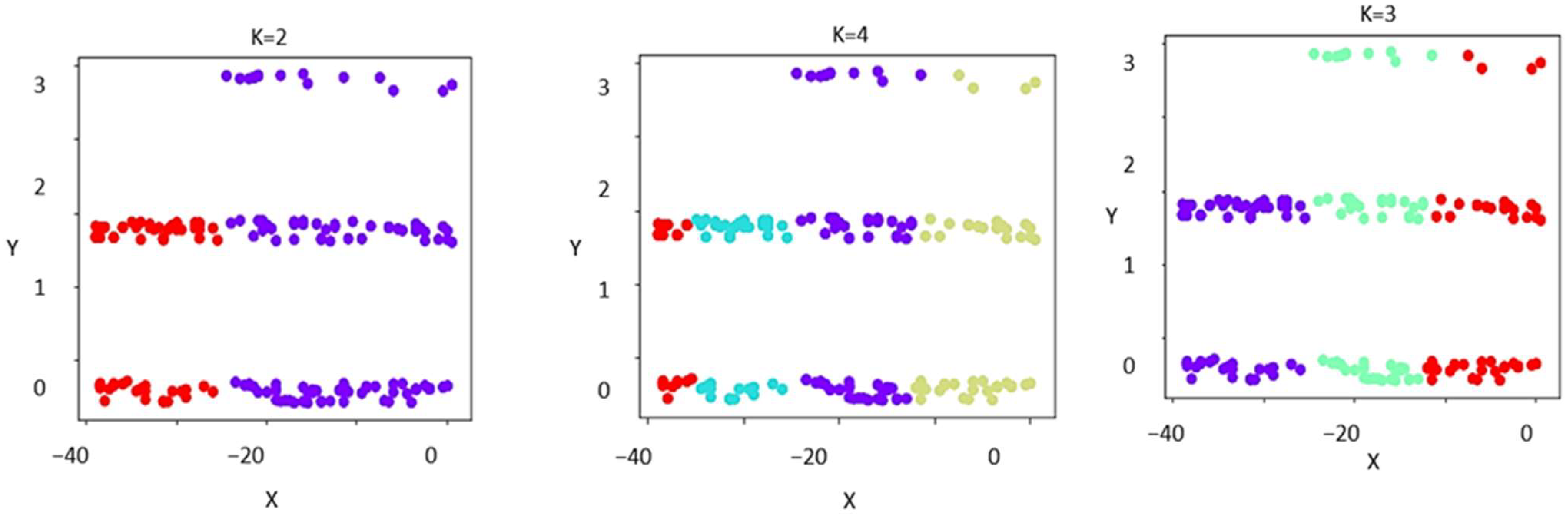
Dendrogram can help decision-makers find out where to stop the clustering algorithm, whether it is an agglomerative or divisive method. Figure 1 shows a graphical view of objectives that are clustered using algorithms.

Different functions for grouping objects may be used depending on the clustering algorithm. While in some methods, the aim is to group the objects with higher similarity, in the other methods, by contrast, the aim might be preventing clustering objects with a high dissimilarity. However, the result will provide a set of clusters where similar objects are grouped to gather. Clustering algorithms can be crisp or fuzzy. However, during the last decades, fuzzy clustering methods have received more attention as they can reflect uncertainties.

Patterns of items will be produced in partitioning methods to place comparable objects closer together (or into any other cost function) into the K partition. Scientists frequently employ the partitioning techniques K-mean, K-medoids and C-mean. A K-means algorithm often seeks out things that are closer to a central point. There will be different partitions depending on how many K points are taken into account. Therefore, figuring out how many partitions to take into account is a crucial first step. The step K-means approach was suggested by Chitta et al. in an effort to determine any relationships between the number and size of the partitions [49]. The Euclidean distance method can be used to determine the distance between two objects with a K centre-point, although other significant metrics, such Manhattan, are frequently utilised when appropriate. Their method is used by Ünler et al. for making partition objects based on the degree of membership [50]. In K-medoids, the number clusters (K) are known a priori. In K-medoids, the number of clusters must be specified before partitioning objects. According to Kaufman et al. (2009), in K-medoids, the benchmark points for calculating the cost (distance) function for each individual item are a set of medoids that will form partitions. The objects are then grouped with a partition, with the partition having the lowest distance function value [51].

P-median problem (PMP) is a mathematical programming method to find the minimum distances between objects:

$$min:{{\displaystyle \sum }}_{i=1}^n{{\displaystyle \sum }}_{j=1}^m{d}_{ij}·X_{ij}$$

(1)

A PMP variation was used by Won et al. [52] to compute similarity coefficients using a machine-component index matrix (MICM). A quick machine localisation approach based on PMP that reduces the differences between centroid and machine locations was discussed by Goldengorin et al. [53]. Krushinsky et al. mentioned that the MCIM matrix’s information is insufficient for providing good layouts [54]. To reduce differences in their research, a novel, simple alternative formulation was applied. Meta-heuristic algorithms have been used to portion or cluster things successfully in specific situations. To increase grouping effectiveness, Paydar et al. suggested using a genetic algorithm with a variable neighbourhood search approach [55].

C-means is another partitioning method that is frequently used in manufacturing problems. In the C-means method, a threshold value is used for determining partitions. The C-means method can be successfully used for reflecting uncertainties. Using the provided data sets, fuzzy c-means algorithms (FCM) often produce a partition matrix. The elements are then assigned to the relevant partition and represented by membership values. M.-S. Yang et al. proposed a modified version of fuzzy C-means that used mixed variable indexes according to MCIM and could consider symbolic and fuzzy variables [56]. Izakian et al. presented a combination of fuzzy C-means and Particle Swarm Optimization, which could easily pass local optimum points [57]. In a cell-forming problem where the clusters are produced based on the cell-size limitation, Oliveira et al. applied a spectral clustering technique to reduce inter-cell movements [58].

Hybrid meta-heuristic algorithms frequently use unsupervised learning techniques. They are typically employed to cluster or split a set of data. Rogers et al. compared the results of a bivariate clustering that applied for small-size problems with a GA, which was used for medium- and large-scale problems where the aim was minimising the sum of dissimilarity measures [59]. Adenso-Diaz et al. presented a 2-phase heuristic-based framework in layout design problems using weighted similarity coefficients [60]. In a factory architecture, Banerjee et al. discussed a two-phase genetic algorithm for creating adaptive clusters and, in turn, detecting bottleneck machines [61]. In a clustering approach, Kao et al. used the ant colony optimisation technique to use agglomerative ants to recognise objects [62]. When grouping objects, F. Yang et al. used a hybrid particle swarm method and KHM technique dubbed PSOKHM to avoid local optimum traps [63]. Then, the material transference issue in manufacturing systems was later addressed by Nouri et al. using the Bacteria Forging Algorithm [64].

Guerrero et al. focused on solving product family and machine grouping problems using a quadratic assignment problem (QAP), where the results were then clustered with a 2-stage Self-Organised Map (SOM) method [65]. The selection of the SOM’s ideal size, according to Chattopadhyay et al., is a significant issue when utilising it [66]. In order to establish the proper size of SOM, they presented a new method that employed the average distortion values during the training phase in SOM as a criterion. To create family problems that might enhance learning processes and provide better patterns, Kuo et al. presented a fuzzy set in a variation of ART [67]. Zdemir et al. concentrated on preventing pointless clusters in the clustering process by employing the proliferation problem in ART [68]. By altering vigilance parameters and training vectors, M.-S. Yang et al. employed a novel technique to enhance the learning process in ART [69]. A novel version of ART that could accept operation sequences and time as inputs was employed by Pandian et al. [70].

The findings of the literature research indicate that learning algorithms have been successfully applied to a variety of supply chain industry issues, making them a viable technology. Additionally, it was discovered that the distribution of products and the recognition of food consumption patterns have not utilised the learning methods. According to what was discovered through reading the articles, the following conclusions were reached: the literature analysis concluded that it is crucial to identify the crucial elements while establishing a new supply chain network. Determining the different product kinds is essential and must be taken into account while establishing a new supply chain. Finding the ideal locations for the supply chain nodes (wholesaler’s centre points) is essential when developing the new supply chain and can reduce transit time and expense. However, learning algorithms were not utilised to convert a local plant into a nationwide supply chain network. Learning algorithms have been widely employed for different engineering issues, including supply chains.

3. Research Methodology

This research proposes a new 3-phase learning approach for supply chains in dynamic product demands (Figure 2).

In the first phase of this research, effective factors of product distribution will be determined using qualitative research. Then in the second phase, using a hybrid agglomerative ward-PCA method, the customers will be divided into an appropriate number of clusters according to the features in the dataset. Then, the appropriate product type will be considered for each cluster based on the clusters that represent their needs.

For this purpose, in phase 3 of the proposed framework, a hybrid agglomerative (PCA-Ward) will be used. The reason for choosing this method is that the PCA method is necessary because of the number of parameters that must be considered in more than two. Moreover, many clustering methods are used to solve the problem and Ward showed better scores in terms of the Silhouette Index and Calinski-Harabasz Index, as discussed in Section 4.

3.1. K-Means Algorithm

As was said in the preceding section, the type of problem must be taken into consideration when selecting an algorithm. Therefore, in this study, we concentrated on the K-means algorithm as the most suitable unsupervised ML method for identifying the best centre points, in accordance with the results of the unsupervised algorithms.

The K-means algorithm was first introduced by [71]. Many scientists regularly utilise this technique, also known as Lloyds’ Algorithm, to solve many computer science and engineering problems, since it is a promising method of clustering the items in a dataset.

The algorithm works by grouping objects into K clusters, with each object going into the cluster with the closest mean. The K-means method calculates the separation between things. In order to attain the smallest squared Euclidean distance, items are to be assigned to clusters. The Euclidean Distance method is the most crucial one for determining how far an object is from the centroid (or centre) of a cluster. However, depending on the type of distances, additional distance algorithms including Euclidean, Manhattan and Cosine are used.

3.2. K-Means Algorithm’s Steps

The K-means algorithm’s steps are as follows:

Step 1: Determine the number of clusters in step one (K).

Step 2: Describe the K-points in step two (or centroids).

Step 3: Determine the separation between each object and its nearest centroid. The predetermined clusters will form (K).

Step 4: By computing the variance values, locate the centroid of each cluster.

Step 5: Return to step 3 and update your distance calculations for each object, taking into account their updated centroid in each cluster.

Step 6: Proceed to step 4 if a new reassignment is possible.

Figure 3 shows an example to clarify how the K-means algorithm clusters data into different groups based on their neighborhood.

A critical point in using the K-means algorithm is determining the number of clusters. Section 4.3.6 will focus more on this point after developing the K-means model.

4. Results and Discussion

In order to conduct the research, a local chocolate manufacturing company located in Kuala Lumpur, Malaysia, is considered. The manufacturer designs and manufactures different products and sells them in all states and federal territories of Malaysia. However, there is no scientific research provided to cluster customers based on their needs and design packages of chocolates accordingly (see Section 2).

4.1. Identifying the Consumers, Availability and Society Factors in Chocolate Consumption (Phase 1)

In order to identify the factors that might influence chocolate consumption in Malaysia, interviews with food industry experts were conducted. Surprisingly, personal factors are not the only factors influencing chocolate consumption. Other than that, society and availability factors are the two main factors that can increase or decrease such consumption. The main factors that affect chocolate consumption are outlined in Figure 4:

The selected factors in Figure 4 will be then considered as the features for the proposed machine learning algorithm (see Section 4.2) to determine the customer clusters based on common needs. Those customers who will be grouped in one cluster will have similar product desires or needs. As a result, the data’s dependent variable (label) will be the “Product Type Desire.”

Using the learning algorithm, we want to know, by considering the personal, societal and availability features, which type of products will be more desired by each customer and then cluster the customer into groups according to their needs and desire.

In order to ascertain data from the statistical society, a questionnaire is designed and distributed into statistical society. The questionnaire is provided in Appendix A.

4.1.1. Level of Chocolate Consumption in Malaysia

The Statistica website indicates that during 2019, Malaysian people spent MYR 4.4 billion on Chocolate and Sugar-based confectionaries (Figure 5).

Each Malaysian paid MYR 137.7 for Chocolate and Sugar-based confectionaries in 2019.

4.4 × 1.000.000.000 RM/31,949,777 (population of Malaysia in the year 2019) = 137.7 RM

(2)

Assuming that half of this value belongs to the chocolate, each Malaysian will spend MYR 68.85 on chocolate products. The in-depth field survey on the internet shows that in the year 2019, the average price of 100 g chocolate bars in the Malaysian market was MYR 14.06 (

Table 1. Data on the Price and Weight of Chocolates in the Malaysian Market.

Brand	Type	Weight (g)	Price (MYR)	Per 100 g (MYR)
1	Ferrero Rocher Chocolate	600	37	6.16
2	Ferrero Rocher Chocolate	38	8.8	23.15
3	Cadbury Dairy Milk Oreo	130	9.9	7.61
4	Nutella B-ready	132	10.8	8.18
5	Ferrero Rocher Chocolate	500	40.9	8.18
6	Cadbury Dairy Milk Oreo	165	8.61	5.21
7	Cadbury Dairy Milk Oreo	160	8.5	5.31
8	Ferrero Rocher Chocolate 3 Pieces	38	8.9	23.42
9	Cadbury Dairy Milk Oreo	90	9.6	10.66
10	Nutella B-ready	132	23.6	17.87
11	Ferrero Rocher Raffaello	50	19.45	38.9
Chocolate Price in the market per 100 g				14.06

):

With MYR 137.7, each Malaysian can eat 980 g of chocolates annually.

Besides, the ministry of foreign affairs of the United States reveals that the average chocolate consumption per capita in the world is 0.9 kg. Compared to the average chocolate consumption globally, Malaysian people usually use chocolate similar to other people worldwide. It is worth knowing that Switzerland people use more than 0.8 kg of chocolate each year. With this amount, we can assume that the portion of using chocolate in Malaysia is normal. Therefore, the average worldwide chocolate consumption per day for each person reported by international statistics can be used as a good ratio for Malaysians. The average daily chocolate usage is 1 billion out of 8 billion. It means that approximately 12.5% of people eat chocolate every day. This ratio can be directly used for Malaysians as they typically consume chocolate (p = 0.125).

4.1.2. Statistical Society

In this section, authentic data is ascertained from society. Since it is impossible to ask all people in Malaysia, it was decided to use statistical society. For this purpose, three major cities in Malaysia are considered the primary target cities: Kula Lumpur, Johor and Penang. Using the Cochran Formula (Equation (3)), the number of statistical societies will be calculated as follows:

The population of States in 2019 that the Ministry of Department Of Statistics Malaysia reports:

W.P Kula Lumpur: 1,778,000 (persons)

Negari Sembilan: 1,132,000 (persons)

Pahang: 1,677,000 (persons)

Total population of the studied area: is 4,587,000 Persons.

$$n=\frac{z_{\frac{\alpha }{2}}^2· p·q+e^2}{\frac{Z_{\frac{\alpha }{2}}^2·p·q}{N}+e^2}=\frac{{\left(1.96\right)}^2· \left(0.5\right)·\left(0.5\right)+{\left(0.05\right)}^2}{\frac{{\left(1.96\right)}^2·\left(0.5\right)·\left(0.5\right)}{4,587,000}+{\left(0.05\right)}^2}=169.06\cong 170$$

(3)

N is the size of the total number of people in the market in Malaysia. p is the portion of that desire to use the chocolate (whether people desire to use chocolate or not); N is the size of the statistical society; e is the tolerable error (0.05) and Z_α/2 is the standard function value. Therefore, the questionnaire will be distributed to 170 people from the studied area.

4.2. Determining the Effective Factors in Chocolate Consumption (Phase 2)

4.2.1. Data Entry

After gathering data on the features of the society, the data are represented in

Table 2. Data Gathered from Society to Determine Product Pattern.

Row	Age	Gender	Education	Diabetics	Health Benefit Awareness	Society Taste	Chocolate Availability	Brand Variety	City
0	79	Male	Below High School Diploma	No	Low	Yes	Medium	Medium	Pahang
1	72	Female	Below High School Diploma	Yes	Low	Yes	Medium	Medium	Sembilan
2	16	Female	High School Diploma	No	High	No	High	High	Kuala Lumpur
3	61	Female	Below High School Diploma	No	Low	No	Medium	Medium	Pahang
4	63	Female	Below High School Diploma	Yes	Low	No	Medium	Medium	Pahang
...	...	...	...	...	...	...	...	...	...
164	16	Male	High School Diploma	No	High	No	High	High	Kuala Lumpur
165	69	Female	High School Diploma	Yes	High	No	Medium	Medium	Sembilan
166	42	Male	Post Graduate	No	Very High	Yes	Medium	Medium	Pahang
167	75	Female	Below High School Diploma	Yes	Low	Yes	Medium	Medium	Sembilan

.

4.2.2. Data Preparation

In order to use data in the proposed algorithm in Python, some qualitative and text data must be changed into the quantitative form. In continuation, the following commands are shown:

• ConsumersData.Gender=ConsumersData.Gender.apply([’Female’,’Male’].index)
• ConsumersData.Education=ConsumersData.Education.apply([’Below High School Diploma’,’High School Diploma’,’University Graduate’,’Post Graduate’].index)
• ConsumersData.Diabetics=ConsumersData.Diabetics.apply([’No’,’Yes’].index)
• ConsumersData.HealthBenefitAwareness=ConsumersData.HealthBenefitAwareness.apply([’Low’,’Medium’,’High’,’Very High’].index)
• ConsumersData.SocietyTaste=ConsumersData.SocietyTaste.apply([’No’,’Yes’].index)
• ConsumersData.ChocolateAvailability=ConsumersData.ChocolateAvailability.apply([’Low’,’Medium’,’High’].index)
• ConsumersData.BrandVariety=ConsumersData.BrandVariety.apply([’Low’,’Medium’,’High’,’Very High’].index)
• ConsumersData.City=ConsumersData.City.apply([’KualaLumpur’,’Sembilan’,’Pahang’].index)

After applying the above commands, the data was prepared in quantitative format (

Table 3. The Transformed Data According to the Preparation Commands in Python.

Row	Age	Gender	Education	Diabetics	Health Benefit Awareness	Society Taste	Chocolate Availability	Brand Variety	City
0	79	1	0	0	0	1	1	1	2
1	72	0	0	1	0	1	1	1	1
2	16	0	1	0	2	0	2	2	0
3	61	0	0	0	0	0	1	1	2
4	63	0	0	1	0	0	1	1	2
...	...	...	...	...	...	...	...	...	...
164	16	1	1	0	2	0	2	2	0
165	69	0	1	1	2	0	1	1	1
166	42	1	3	0	3	1	1	1	2
167	75	0	0	1	0	1	1	1	1
168	68	1	1	0	2	1	1	1	1

).

4.2.3. Descriptive Analysis

In this section, the gathered data will be analysed using the statistical library in Python. This section shows that data are generally distributed between males and females. Moreover, more than 70% of the society are highly educated and only 21% are Diabetics. However, unfortunately, statistical society is now aware enough of the role of chocolate in health (1.22 out of 4), and chocolate availability is good enough in their region, as they desired; however, there is still space to bring new brands (1.27 out of 2) (

Table 4. The Descriptive Analysis of the Data in the Society.

	Row	Age	Gender	Education	Diabetics	Health Benefit Awareness	Society Taste	Chocolate Availability	Brand Variety	City
count	169.00	169.00	169.00	169.00	169.00	169.00	169.00	169.00	169.00	169.00
mean	85.00	38.781	0.432	0.745	0.213	1.224	0.289	1.272	1.272	1.082
std	48.930	23.373	0.496	0.852	0.411	1.105	0.455	0.446	0.446	0.789
min	1.00	1.00	0.00	0.00	0.00	0.00	0.00	1.00	1.00	0.00
25%	43.00	17.00	0.00	0.00	0.00	0.00	0.00	1.00	1.00	0.00
50%	85.00	39.00	0.00	1.00	0.00	2.00	0.00	1.00	1.00	1.00
75%	127.00	56.00	1.00	1.00	0.00	2.00	1.00	2.00	2.00	2.00

).

4.2.4. Determining the Effective Factors Using Shapiro Ranking Method

This section will identify the effective factors using the Shapiro ranking method in the Yellowbrick library. The aim is to find which factors are effective in the training process. If a factor is ineffective, it can be removed from training processing. Figure 6 indicates that all factors are effective and shall not be ignored during the process.

4.3. Using a Hybrid PCA and Ward Agglomerative Clustering Method for Consumption Pattern (Phase 3)

After determining the data for the product type desired, the cluster of customers in terms of the features can be figured out. Moreover, the pattern of product desire for the rest of the cities in Malaysia can be determined. Since we do not know the number of product types to be prepared for the markets, it is better to use Agglomerative Clustering methods to specify the number of clusters (people groups) according to their features. Then, for each cluster, a specific product type could be prepared. This section aims to find the customers that can be divided into a certain number of clusters. Then, a particular type (or a package) of chocolate(s) can be considered for each cluster.

The necessary steps to develop the solving algorithm used in phases 2 and 3 of the framework will be shown (Figure 7).

Python was utilised in this study to code the suggested algorithm. One of the most popular programmes with a potent engine for calculating mathematical equations and models is Python. There are various uses for Python. Jupyter is a useful platform for creating algorithms since it allows each line of script to be run independently and display the results. In this research, a personal laptop with Windows 10 Enterprise, Intel Core i7, 4 GB VGA, 8 GB RAM was used.

4.3.1. Libraries

The libraries that should be imported to Python to be used in this section are as follows:

• from sklearn import linear_model
• from sklearn import cluster, datasets
• import numpy as np
• import pandas as pd
• from math import sqrt
• import scipy.cluster.hierarchy as shc
• from sklearn.preprocessing import StandardScaler
• from sklearn.decomposition import PCA
• from mlxtend.plotting import plot_decision_regions
• import matplotlib.pyplot as plt
• import matplotlib.gridspec as gridspec
• import itertools
• from sklearn.metrics import silhouette_score

4.3.2. Using PCA Method

In this method, the ten features are considered. However, a PCA method should be considered to consider all features in the dataset.

pca = PCA (n_components = 2)

(4)

X = pca.fit_transform (X)

(5)

w2.fit (X)

(6)

After using PCA method, the data in 10 features will be downsized to the 2 dummy features:

array([[40.21847836, −1.34506094],

[33.22742738, −1.39573043],

[−22.78335868, 0.65705467],

[22.22322185, −1.35425239],

[24.22312134, −1.35532962],

[−31.78233389, −1.31869809],

[31.21332019, −1.44789902],

[−19.78296358, 0.86418076],

[12.2193131, 0.65062064],

…

[3.22312041, 2.85635524],

[36.21900695, −1.39087729],

[29.21857854, 0.77858665]])

4.3.3. Determining the Appropriate Number of Clusters Using a Dendrogram

One way to recognise the appropriate number of clusters (K) is to use a Dendrogram. A dendrogram is an agglomerative method for clustering data. In the dendrogram, the correct number of clusters can be estimated by looking at long vertical lines.

A horizontal cut in Figure 8 where the vertical lines have long distances, shows that the correct number of clusters could be 2 or 3. The correct value for the number of clusters will be outlined using some learning algorithms metrics.

4.3.4. Training the Agglomerative Algorithm

In this section, it is time to train the model for the datasets. For this purpose, three models will be used where the Ward linkage method is used. The reason for choosing the Ward method is that Ward is the most frequently applied method for linkage clusters in the literature. In Python, the default linkage method is also Ward. While using Ward, the Euclidean Method for measuring the pairwise distances is used. In each model, number clusters are considered 3 and 5, respectively.

w2 = cluster.AgglomerativeClustering(n_clusters=2,linkage=‘ward’).fit(X)

(7)

w3 = cluster.AgglomerativeClustering(n_clusters=3,linkage=‘ward’).fit(X)

(8)

w4 = cluster.AgglomerativeClustering(n_clusters=4,linkage=‘ward’).fit(X)

(9)

Figure 9 shows the clustering scatter chart based on the Ward method and a predefined number of clusters. In this figure, each cluster group of members with similar features is shown by a color (red, purple, etc.). As seen, while the number of clusters is considered 3, the proposed algorithm could specify the clusters more precisely. In the right image, it is unnecessary to separate the red clusters from the main cluster.

4.3.5. Silhouette Coefficient

The Silhouette Coefficient is an index used to measure the quality of the clustering method [72]. The higher the Silhouette value for a method means that the algorithm could separate clusters more accurately and, consequently, the number of clusters is selected precise.

The Silhouette indicator is defined as below:

$$S_i=\frac{x_i-y_i}{max\left\{x_i,y_i\right\}}$$

(10)

where y_i is the average distance between point I and all other points in its cluster and x_i is the shortest average distance of point I to all other points in any other cluster.

The outcomes show that while the number of clusters is considered 3 (K = 3), better Silhouette values for the agglomerative values will be observed (Figure 10). In this figure, squares indicate the number of clusters and circles show the fitness time spent for calculating silhouette score for each cluster.

4.3.6. Calinski-Harabasz Index

If the clusters are very compact and, at the same time, they are well-spaced from each other, then the Calinski-Harabasz Index would be higher. Based on the variance of the sums of squares of the individual object distances from their cluster centres, the Calinski-Harabasz Index operates:

$$C{H}_k=\frac{SSB}{k-1}·\frac{n-k}{SSW}$$

(11)

k is the number of clusters, n is the number of records in the data and SSW is the overall within-cluster variance. SSB is the overall between-cluster variance. The results of the Calinski-Harabasz Index for the studied agglomerative clustering algorithm are shown in Figure 11:

Figure 11 shows that for the models (K = 2 and K = 3), the Calinski-Harabsaz Graph shows that the best score is achieved while the number of clusters is considered 3. As a result, the number of clusters for the food supply chain should be 3, meaning there are 3 main groups of customers that must be prepared based on their needs.

5. Conclusions

This research proposes a 3-phase learning-based framework for making a local factory in Malaysia into a nationwide supply chain. In the first stage of this research, effective factors for product classification according to Malaysia’s features are identified. For this purpose, some factors are identified using the literature review outcomes, statistical information from the food research institute and interviews with academic and industry experts. Then, using a questionnaire, the following factors are identified as the influential factors for the chocolate consumption pattern that can be used for clustering the product types in phase 3:

• Availability Factors: Chocolate Availability, Brand Variety
• Society Factors: Health benefit Awareness, Society Taste (Desire)
• Consumer’s Factors: Age, Gender, Education, Diabetic Status

The outcomes of this section gathered from 169 responders from the society show that data are normally distributed between males and females. Moreover, more than 70% of the society is highly educated and only 21% are Diabetics. However, unfortunately, statistical society is now aware of the role of chocolate in health (1.22 out of 4) and chocolate availability is good enough in their region as desired; however, there is still space to bring new brands (1.27 out of 2). The outcomes of using the hybrid PCA and Agglomerative Clustering Method showed that according to the gathered data, there are three main clusters of using products (three main groups). This information can help managers of the local factory know the national pattern of using chocolates. As a result, they can prepare products according to the consumer’s desire. Further expanding the model using fuzzy systems to consider the uncertainty of factors (features) in product type patterns is recommended.

References

1. Fornasiero, R.; Macchion, L.; Vinelli, A. Supply chain configuration towards customization: A comparison between small and large series production. IFAC-PapersOnLine 2015, 48, 1428–1433. [Google Scholar] [CrossRef]
2. Şen, A. The US fashion industry: A supply chain review. Int. J. Prod. Econ. 2008, 114, 571–593. [Google Scholar] [CrossRef] [Green Version]
3. Montagna, G. Multi-dimensional consumers: Fashion and human factors. Procedia Manuf. 2015, 3, 6550–6556. [Google Scholar] [CrossRef]
4. Delgado, M.J.B.L.; Albuquerque, M.H.F. The contribution of regional costume in fashion. Procedia Manuf. 2015, 3, 6380–6387. [Google Scholar] [CrossRef] [Green Version]
5. Iannone, R.; Martino, G.; Miranda, S.; Riemma, S. Modeling fashion retail supply chain through causal loop diagram. IFAC-PapersOnLine 2015, 48, 1290–1295. [Google Scholar] [CrossRef]
6. Macchion, L.; Moretto, A.; Caniato, F.; Caridic, M.; Danese, P.; Vinelli, A. Production and supply network strategies within the fashion industry. Int. J. Prod. Econ. 2015, 163, 173–188. [Google Scholar] [CrossRef]
7. Pishvaee, M.S.; Jolai, F.; Razmi, J. A stochastic optimization model for integrated forward/reverse logistics network design. J. Manuf. Syst. 2009, 28, 107–114. [Google Scholar] [CrossRef]
8. Zilberman, D.; Lu, L.; Reardon, T. Innovation-induced food supply chain design. Food Policy 2019, 83, 289–297. [Google Scholar] [CrossRef]
9. Caniato, F.; Caridi, M.; Moretto, A.; Sianesi, A.; Spina, G. Integrating international fashion retail into new product development. Int. J. Prod. Econ. 2014, 147, 294–306. [Google Scholar] [CrossRef]
10. El-Baz, M.A. Fuzzy performance measurement of a supply chain in manufacturing companies. Expert Syst. Appl. 2011, 38, 6681–6688. [Google Scholar] [CrossRef]
11. Olugu, E.U.; Wong, K.Y. An expert fuzzy rule-based system for closed-loop supply chain performance assessment in the automotive industry. Expert Syst. Appl. 2012, 39, 375–384. [Google Scholar] [CrossRef]
12. Chen, J.-M.; Chang, C.-I. Dynamic pricing for new and remanufactured products in a closed-loop supply chain. Int. J. Prod. Econ. 2013, 146, 153–160. [Google Scholar] [CrossRef]
13. Mehrjoo, M.; Pasek, Z.J. Impact of product variety on supply chain in fast fashion apparel industry. Procedia CIRP 2014, 17, 296–301. [Google Scholar] [CrossRef] [Green Version]
14. Zhou, E.; Zhang, J.; Gou, Q.; Liang, L. A two period pricing model for new fashion style launching strategy. Int. J. Prod. Econ. 2015, 160, 144–156. [Google Scholar] [CrossRef]
15. Yang, S.; Xiao, Y.; Kuo, Y.-H. The supply chain design for perishable food with stochastic demand. Sustainability 2017, 9, 1195. [Google Scholar] [CrossRef] [Green Version]
16. Soolaki, M.; Arkat, J. Incorporating dynamic cellular manufacturing into strategic supply chain design. Int. J. Adv. Manuf. Technol. 2018, 95, 2429–2447. [Google Scholar] [CrossRef]
17. Allaoui, H.; Guo, Y.; Choudhary, A.; Bloemhof, J. Sustainable agro-food supply chain design using two-stage hybrid multi-objective decision-making approach. Comput. Oper. Res. 2018, 89, 369–384. [Google Scholar] [CrossRef] [Green Version]
18. Cohen, M.A.; Lee, H.L. Designing the right global supply chain network. Manuf. Serv. Oper. Manag. 2020, 22, 15–24. [Google Scholar] [CrossRef] [Green Version]
19. Mogale, D.; Kumar, S.K.; Tiwari, M.K. Green food supply chain design considering risk and post-harvest losses: A case study. Ann. Oper. Res. 2020, 295, 257–284. [Google Scholar] [CrossRef]
20. Singh, S.; Kumar, R.; Panchal, R.; Tiwari, M.K. Impact of COVID-19 on logistics systems and disruptions in food supply chain. Int. J. Prod. Res. 2021, 59, 1993–2008. [Google Scholar] [CrossRef]
21. Ni, Y.; Fan, F. A two-stage dynamic sales forecasting model for the fashion retail. Expert Syst. Appl. 2011, 38, 1529–1536. [Google Scholar] [CrossRef]
22. Wang, S.-P.; Lee, W.; Chang, C.-Y. Modeling the consignment inventory for a deteriorating item while the buyer has warehouse capacity constraint. Int. J. Prod. Econ. 2012, 138, 284–292. [Google Scholar] [CrossRef]
23. Lo, C.K.; Yeung, A.C.; Cheng, T. The impact of environmental management systems on financial performance in fashion and textiles industries. Int. J. Prod. Econ. 2012, 135, 561–567. [Google Scholar] [CrossRef]
24. Dye, C.-Y.; Hsieh, T.-P. An optimal replenishment policy for deteriorating items with effective investment in preservation technology. Eur. J. Oper. Res. 2012, 218, 106–112. [Google Scholar] [CrossRef]
25. Basu, P.; Nair, S.K. A decision support system for mean–variance analysis in multi-period inventory control. Decis. Support Syst. 2014, 57, 285–295. [Google Scholar] [CrossRef]
26. Zhao, F.; Hong, Y.; Yu, D.; Yang, Y.; Zhang, Q. A hybrid particle swarm optimisation algorithm and fuzzy logic for process planning and production scheduling integration in holonic manufacturing systems. Int. J. Comput. Integr. Manuf. 2010, 23, 20–39. [Google Scholar] [CrossRef]
27. Delgoshaei, A.; Ali, A.; Khairol, M.; Ariffin, A.; Gomes, C. A multi-period scheduling of dynamic cellular manufacturing systems in the presence of cost uncertainty. Comput. Ind. Eng. 2016, 100, 110–132. [Google Scholar] [CrossRef]
28. Delgoshaei, A.; Ariffin, M.K.A.; Ali, A. A multi-period scheduling method for trading-off between skilled-workers allocation and outsource service usage in dynamic CMS. Int. J. Prod. Res. 2017, 55, 997–1039. [Google Scholar] [CrossRef]
29. Novák, V.; Perfilieva, I.; Mockor, J. Mathematical Principles of Fuzzy Logic; Springer Science & Business Media: Berlin, Germany, 2012; Volume 517. [Google Scholar]
30. Regulwar, D.G.; Gurav, J.B. Irrigation planning under uncertainty—A multi objective fuzzy linear programming approach. Water Resour. Manag. 2011, 25, 1387–1416. [Google Scholar] [CrossRef]
31. Liang, T.-F.; Cheng, H.-W.; Chen, P.-Y.; Shen, K.-H. Application of fuzzy sets to aggregate production planning with multiproducts and multitime periods. IEEE Trans. Fuzzy Syst. 2011, 19, 465–477. [Google Scholar] [CrossRef]
32. Jia, G.; Bai, M. An approach for manufacturing strategy development based on fuzzy-QFD. Comput. Ind. Eng. 2011, 60, 445–454. [Google Scholar] [CrossRef]
33. Lootsma, F.A. Fuzzy Logic for Planning and Decision Making; Springer Science & Business Media: Berlin, Germany, 2013; Volume 8. [Google Scholar]
34. Govindan, K.; Mina, H.; Esmaeili, A.; Gholami-Zanjani, S.M. An integrated hybrid approach for circular supplier selection and closed loop supply chain network design under uncertainty. J. Clean. Prod. 2020, 242, 118317. [Google Scholar] [CrossRef]
35. Mula, J.; Peidro, D.; Poler, R. The effectiveness of a fuzzy mathematical programming approach for supply chain production planning with fuzzy demand. Int. J. Prod. Econ. 2010, 128, 136–143. [Google Scholar] [CrossRef]
36. Qin, Z.; Bai, M.; Ralescu, D. A fuzzy control system with application to production planning problems. Inf. Sci. 2011, 181, 1018–1027. [Google Scholar] [CrossRef]
37. MacCarthy, B.L.; Jayarathne, P. Supply network structures in the international clothing industry: Differences across retailer types. Int. J. Oper. Prod. Manag. 2013, 33, 858–886. [Google Scholar] [CrossRef]
38. Delgoshaei, A.; Ariffin, M.K.A.M.; Leman, Z.; Baharudin, B.T.H.T.B.; Gomes, G. Review of evolution of cellular manufacturing system’s approaches: Material transferring models. Int. J. Precis. Eng. Manuf. 2016, 17, 131–149. [Google Scholar] [CrossRef]
39. Paciarotti, C.; Torregiani, F. The logistics of the short food supply chain: A literature review. Sustain. Prod. Consum. 2020, 26, 422–428. [Google Scholar] [CrossRef]
40. Macchion, L.; Moretto, A.; Caniato, F.; Caridi, M.; Danese, P.; Spina, G.; Vinelli, A. Improving innovation performance through environmental practices in the fashion industry: The moderating effect of internationalisation and the influence of collaboration. Prod. Plan. Control 2017, 28, 190–201. [Google Scholar] [CrossRef]
41. Levner, E.; Proth, J.-M. Strategic management of ecological systems: A supply chain perspective. In Strategic Management of Marine Ecosystems; Springer: Berlin, Germany, 2005; pp. 95–107. [Google Scholar]
42. Levner, E. Risk/Cost Analysis of Sustainable Management of Wastewater for Irrigation: Supply Chain Approach. In Wastewater Reuse–Risk Assessment, Decision-Making and Environmental Security; Springer: Berlin, Germany, 2007; pp. 33–42. [Google Scholar]
43. Nagurney, A.; Yu, M. Sustainable fashion supply chain management under oligopolistic competition and brand differentiation. Int. J. Prod. Econ. 2012, 135, 532–540. [Google Scholar] [CrossRef]
44. Yang, L.; Ng, C.T. Flexible capacity strategy with multiple market periods under demand uncertainty and investment constraint. Eur. J. Oper. Res. 2014, 236, 511–521. [Google Scholar] [CrossRef]
45. Lion, A.; Macchion, L.; Danse, P.; Vinelli, A. Sustainability approaches within the fashion industry: The supplier perspective. In Supply Chain Forum: An International Journal; Taylor & Francis: Oxford, OH, USA, 2016. [Google Scholar]
46. Macchion, L.; Da Giau, A.; Caniato, F.; Caridi, M.; Danese, P.; Rinaldi, R.; Vinelli, A. Strategic approaches to sustainability in fashion supply chain management. Prod. Plan. Control 2018, 29, 9–28. [Google Scholar] [CrossRef]
47. Moretto, A.; Macchion, L.; Lion, A.; Caniato, F.; Danese, P.; Vinelli, A. Designing a roadmap towards a sustainable supply chain: A focus on the fashion industry. J. Clean. Prod. 2018, 193, 169–184. [Google Scholar] [CrossRef]
48. Theodoridis, S.; Pikrakis, A.; Koutroumbas, K.; Cavouras, D. Introduction to Pattern Recognition: A Matlab Approach: A Matlab Approach; Access Online via Elsevier: Amsterdam, The Netherlands, 2010. [Google Scholar]
49. Chitta, R.; Murty, M.N. Two-level k-means clustering algorithm for kτ relationship establishment and linear-time classification. Pattern Recognit. 2010, 43, 796–804. [Google Scholar] [CrossRef]
50. Ünler, A.; Güngör, Z. Applying K-harmonic means clustering to the part-machine classification problem. Expert Syst. Appl. 2009, 36, 1179–1194. [Google Scholar] [CrossRef]
51. Kaufman, L.; Rousseeuw, P.J. Finding Groups in Data: An Introduction to Cluster Analysis; Wiley Com: Hoboken, NJ, USA, 2009; Volume 344. [Google Scholar]
52. Won, Y.; Currie, K.R. An effective p-median model considering production factors in machine cell/part family formation. J. Manuf. Syst. 2006, 25, 58–64. [Google Scholar] [CrossRef]
53. Goldengorin, B.; Krushinsky, D.; Slomp, J. Flexible PMP approach for large-size cell formation. Oper. Res. 2012, 60, 1157–1166. [Google Scholar] [CrossRef] [Green Version]
54. Krushinsky, D.; Goldengorin, B. An exact model for cell formation in group technology. Comput. Manag. Sci. 2012, 9, 323–338. [Google Scholar] [CrossRef] [Green Version]
55. Paydar, M.M.; Saidi-Mehrabad, M. A hybrid genetic-variable neighborhood search algorithm for the cell formation problem based on grouping efficacy. Comput. Oper. Res. 2013, 40, 980–990. [Google Scholar] [CrossRef]
56. Yang, M.-S.; Hung, W.-L.; Cheng, F.-C. Mixed-variable fuzzy clustering approach to part family and machine cell formation for GT applications. Int. J. Prod. Econ. 2006, 103, 185–198. [Google Scholar] [CrossRef]
57. Izakian, H.; Abraham, A. Fuzzy C-means and fuzzy swarm for fuzzy clustering problem. Expert Syst. Appl. 2011, 38, 1835–1838. [Google Scholar] [CrossRef]
58. Oliveira, S.; Ribeiro, J.; Seok, S. A spectral clustering algorithm for manufacturing cell formation. Comput. Ind. Eng. 2009, 57, 1008–1014. [Google Scholar] [CrossRef]
59. Rogers, D.F.; Kulkarni, S.S. Optimal bivariate clustering and a genetic algorithm with an application in cellular manufacturing. Eur. J. Oper. Res. 2005, 160, 423–444. [Google Scholar] [CrossRef]
60. Adenso-Diaz, B.; Lozano, S.; Eguía, I. Part-machine grouping using weighted similarity coefficients. Comput. Ind. Eng. 2005, 48, 553–570. [Google Scholar] [CrossRef]
61. Banerjee, I.; Das, P. Group technology based adaptive cell formation using predator–prey genetic algorithm. Appl. Soft Comput. 2012, 12, 559–572. [Google Scholar] [CrossRef]
62. Kao, Y.; Li, Y. Ant colony recognition systems for part clustering problems. Int. J. Prod. Res. 2008, 46, 4237–4258. [Google Scholar] [CrossRef]
63. Yang, F.; Sun, T.; Zhang, C. An efficient hybrid data clustering method based on K-harmonic means and Particle Swarm Optimization. Expert Syst. Appl. 2009, 36, 9847–9852. [Google Scholar] [CrossRef]
64. Nouri, H.; Tang, S.H.; Hang Tuan, B.T.; Anura, M.K. BASE: A bacteria foraging algorithm for cell formation with sequence data. J. Manuf. Syst. 2010, 29, 102–110. [Google Scholar] [CrossRef]
65. Guerrero, F.; Lozano, S.; Smith, K.A.; Canca, D.; Kwok, T. Manufacturing cell formation using a new self-organizing neural network. Comput. Ind. Eng. 2002, 42, 377–382. [Google Scholar] [CrossRef]
66. Chattopadhyay, M.; Dan, P.K.; Mazumdar, S. Application of visual clustering properties of self organizing map in machine–part cell formation. Appl. Soft Comput. 2012, 12, 600–610. [Google Scholar] [CrossRef] [Green Version]
67. Kuo, R.J.; Su, Y.T.; Chiu, C.Y.; Chen, K.-Y.; Tien, F.C. Part family formation through fuzzy ART2 neural network. Decis. Support Syst. 2006, 42, 89–103. [Google Scholar] [CrossRef]
68. Özdemir, R.G.; Gençyılmaz, G.; Aktin, T. The modified fuzzy art and a two-stage clustering approach to cell design. Inf. Sci. 2007, 177, 5219–5236. [Google Scholar] [CrossRef]
69. Yang, M.-S.; Yang, J.-H. Machine-part cell formation in group technology using a modified ART1 method. Eur. J. Oper. Res. 2008, 188, 140–152. [Google Scholar] [CrossRef]
70. Pandian, R.S.; Mahapatra, S.S. Manufacturing cell formation with production data using neural networks. Comput. Ind. Eng. 2009, 56, 1340–1347. [Google Scholar] [CrossRef]
71. MacQueen, J. Some methods for classification and analysis of multivariate observations. In Proceedings of the Fifth Berkeley Symposium on Mathematical Statistics and Probability, Oakland, CA, USA, 21 June 1967. [Google Scholar]
72. Kaoungku, N.; Suksu, K.; Chanklan, R.; Kerdprasop, K.; Kerdprasop, N. The silhouette width criterion for clustering and association mining to select image features. Int. J. Mach. Learn. Comput. 2018, 8, 69–73. [Google Scholar] [CrossRef] [Green Version]
Figure 1. Graphical view of cluster simulating.
Mathematics 11 01085 g001
Figure 2. Block diagram of the proposed 3-phase algorithm.
Mathematics 11 01085 g002
Figure 3. Using the K-means algorithm in clustering data into five clusters.
Mathematics 11 01085 g003
Figure 4. Selected Features for Determining the Client Pattern.
Mathematics 11 01085 g004
Figure 5. The graph of sold chocolate in Malaysia (Source: Statistica website).
Mathematics 11 01085 g005
Figure 6. Shapiro Ranking Chart for Determining the Effective Features.
Mathematics 11 01085 g006
Figure 7. Steps for developing the proposed algorithm.
Mathematics 11 01085 g007
Figure 8. Dendrogram of the Clustered Data.
Mathematics 11 01085 g008
Figure 9. The Agglomerative Clustering Algorithm Result While the Number of Clusters is considered 2, 3 and 4.
Mathematics 11 01085 g009
Figure 10. Silhouette Graph for the Agglomerative Clustering Method while K = 2, 3 and 4, respectively.
Mathematics 11 01085 g010
Figure 11. Calinski-Harabasz Graph for the Agglomerative Clustering Method while K = 2, 3 and 4, respectively.
Mathematics 11 01085 g011