Fusion and Allocation Network for Light Field Image Super-Resolution

Abstract

Light field (LF) images taken by plenoptic cameras can record spatial and angular information from real-world scenes, and it is beneficial to fully integrate these two pieces of information to improve image super-resolution (SR). However, most of the existing approaches to LF image SR cannot fully fuse the information at the spatial and angular levels. Moreover, the performance of SR is hindered by the ability to incorporate distinctive information from different views and extract informative features from each view. To solve these core issues, we propose a fusion and allocation network (LF-FANet) for LF image SR. Specifically, we have designed an angular fusion operator (AFO) to fuse distinctive features among different views, and a spatial fusion operator (SFO) to extract deep representation features for each view. Following these two operators, we further propose a fusion and allocation strategy to incorporate and propagate the fusion features. In the fusion stage, the interaction information fusion block (IIFB) can fully supplement distinctive and informative features among all views. For the allocation stage, the fusion output features are allocated to the next AFO and SFO for further distilling the valid information. Experimental results on both synthetic and real-world datasets demonstrate that our method has achieved the same performance as state-of-the-art methods. Moreover, our method can preserve the parallax structure of LF and generate faithful details of LF images.

1. Introduction

Compared with conventional cameras, light field (LF) cameras can record the 4D information of a scene in a single shot. The principles of an LF camera are simply illustrated in Figure 1a,b. This LF imaging technology is promising and is successfully used in many applications, such as VR [1], 3D reconstruction [2] and salience detection [3]. However, due to the fixed resolution of imaging sensors, spatial and angular resolutions are a trade-off problem, which leads to each sub-aperture image (SAI) having a lower resolution under the more angular information. This problem leads to performance degradation in the field of their applications. Consequently, LF image super-solution (SR) algorithms have been widely investigated to obtain high-resolution (HR) LF images.

The SAIs captured by the LF camera can record the complex parallax structure of LF, which is displayed in Figure 1c. Each SAI has a high correlation with slight differences among different views, which is the key difference from the case in single image SR (SISR) methods. Most classic traditional algorithms [4,5,6,7,8] achieve SR LF images by using disparity information. This estimated disparity information is utilized to explore the correlation among SAIs. However, the reconstruction quality is quite impacted by the inaccurate disparity. Although traditional methods relying on the disparity have been continuously investigated, obtaining accurate disparity is still a key concern to be addressed.

With the development of deep learning, learning-based methods have been successfully applied in single image SR (SISR). Although some SISR methods [9,10,11] can directly be used in SR for each SAI, these methods destroy the parallax structural properties of LF. Recently, some LF image SR methods [12,13,14,15,16,17,18,19] have been continually proposed to improve the performance of LF image SR and preserve the 4D LF structure. Wang et al. [12] proposed the LFNet to stack SAIs to reconstruct HR SAIs. Only the horizontal and vertical structure of LF views was preserved in this structure. To increase the angular corrections among SAIs, Zhang et al. [13] proposed the resLF, which utilized two more directions than LFNet. However, the SR center view information is not fully supplemented by all auxiliary views. Recently, Jin et al. [14] proposed an all-to-one model (ATO) to generate one SR reference view, and a structural consistency regularization was proposed to maintain the structure of HR space. Moreover, Wang et al. [15] directly utilized micro-pixel images to extract the information of angular and spatial dimensions, whose core components are two types of convolutions with different kernel sizes. More recently, Wang et al. [16] used a deformable convolution network to align the reference information and side-view information among LF. Due to the successful application of 3D convolution in video SR, Liu et al. [20] proposed an LF-IINet to investigate intra-inter view information based on the 3D convolution. In summary, these methods continually improve the utilization of spatial and angular information and have excellent performance. However, there are still two problems left, which have not been well solved among these methods. One is that the spatial and angular information is usually treated uniformly, which destroys the spatial and angular information-independent properties; another is how to effectively fuse and allocate the complementary information from different SAIs.

In order to handle these issues, we propose a fusion and allocation network (namely, LF-FANet) for achieving LF image SR. Our method can effectively and efficiently fuse and allocate complementary information in angular and spatial dimensions. Given a low-resolution (LR) LF image, two dense atrous spatial pyramid poolings (DASPPs) are used to extract initial features. Then, we propose an angular fusion operator (AFO) and a spatial fusion operator (SFO) to capture the inter-view correlation among all views and extract the deep representation of each view, respectively. To preserve the parallax structure of LF images, a key strategy is proposed that consists of two stages, fusion and allocation. Specifically, the outputs of AFO and SFO are fed into the interaction information fusion block (IIFB). This block can preserve the structural properties among LF views in the first stage by fully utilizing spatial and angular correlations. After that, the fusion feature is distributed to another pair of AFO and SFO to further generate informative features for spatial and angular dimensions on their own branch. This allocation stage can separately process spatial and angular features, which makes LF representation learning easier. Based on this strategy, our LF-FANet can fully utilize the spatial information of each SAI and angular correlation among all LF images. The experimental results on real-world and synthetic datasets demonstrate that the performance of our LF-FANet achieves a state-of-the-art performance and preserves structural consistency. The main contributions of this paper are listed as follows.

• We propose two operators (AFO and SFO), which can equally extract and fuse spatial and angular features. The AFO models the correlations among all views in angular subspace, and the SFO models the spatial information of each view in space subspace. Note that the designed AFO and SFO can be regarded as generic modules to use in other LF works (e.g., LF depth estimation and LF segmentation), which are effective at extracting angular and spatial information.
• We propose a fusion and allocation strategy to aggregate and distribute the fusion features. Based on this strategy, our method can effectively exploit spatial and angular information from all LF views. Meanwhile, this strategy can provide more informative features for the next AFO and SFO. Our strategy can not only generate high-quality reconstruction results but also preserve LF structural consistency.
• Our LF-FANet is an end-to-end network for LF image SR, which has significantly improved compared with the state-of-the-art methods developed in recent years.

The rest of this paper is organized into the following sections. Section 2 introduces a brief overview of the related work. Section 3 mainly describes the architecture of our LF-FANet. In Section 4, we provide comparative experiments and ablation studies by using synthetic and real-world datasets. Finally, Section 5 summarizes the conclusion of this paper.

2. Related Work

In this section, we first review the existing single-image SR algorithms. Then, some LF image SR algorithms are briefly covered.

2.1. Single Image SR

Given a low-resolution (LR) image, the single image SR (SISR) is a general task to reconstruct one faithful image with high-resolution (HR). In order to achieve this task, many algorithms based on deep learning have been employed. Here, we only describe a few significant works in this literature. Dong et al. [9,21] proposed a seminal network (SRCNN), which utilized the powerful representation capability of CNN to achieve SISR. By far, many variants of CNN-based networks still dominated this field. Kim et al. [10] proposed a residual learning network (VDSR), which mainly learned high-frequency residual information. Mao et al. [22] proposed a very deep fully convolution-deconvolution network (RED), which was an encoding-decoding framework to learn the mapping relationship from LR images to SR images. Tong et al. [23] proposed a dense skip connections network (SRDenseNet), which effectively combined the low-level features and high-level features to promote the process of reconstruction. Lim et al. [11] proposed an enhanced deep SR network (EDSR), which contained the local and global residual connections. Recently, many SR networks with attention mechanisms have achieved a superior performance. Zhang et al. [24] proposed a residual channel attention network (RCAN), which inserted a channel attention module for considering the interdependence among channels. Dai et al. [25] proposed a second-order attention network (SAN), which employed the trainable second-order attention module to capture spatial information. Both the RCAN and SAN have achieved promising performances in the task of SISR.

To summarize, SISR networks with different structures of deep CNNs can gradually improve the utilization of spatial information in a single image. It should be noted that, although fine-tuning the SISR is a straightforward way to achieve LF image SR, the performance of these methods is hindered due to the lack of angular information.

2.2. LF Image SR

Similar to SISR, LF image SR is still an ill-posed inverse problem, which learns the non-linear mapping from LR SAIs to HR SAIs. However, SAIs captured by an LF camera contain rich angular information, which can be used to improve the performance of LF Image SR. Existing methods can be mainly divided into two categories: explicit-based and implicit-based methods.

2.2.1. Explicit-Based Methods

Explicit-based approaches reconstruct SR images through the estimated disparities, which are explicit information for LF image reconstruction. Bishop and Favaro [4] proposed an explicit image formation model via depth estimation, which used a Bayesian framework to reconstruct LF images. Wanner and Goldluecke [5,6] proposed a variational optimization algorithm to generate HR SAIs. These methods compute the disparity map on the epipolar images (EPIs). Mitra and Veeraraghavan [7] proposed a patch-based approach to address the problem of LF image SR, which used a Gaussian mixture model to estimate disparity. Rossi and Frossard [8] proposed a graph regularizer for LF image SR, based on the coarse disparities. In summary, all of these methods reconstruct the 4D LF by relying on the disparity estimation. However, it is difficult to calculate the accurate disparity along occlusion boundaries and it is harmful to reconstruct high-quality images with erroneous estimation.

2.2.2. Implicit-Based Methods

With the development of deep learning, many methods implicitly learn the mapping relationship between LR SAIs and HR SAIs. These methods have gradually come into the spotlight. Yoon et al. [26] proposed an early CNN-based network (LFCNN), which could simultaneously enhance angular and spatial resolution. Inspired by the structure of recurrent neural networks, Wang et al. [12] designed a bidirectional recurrent CNN network (LFNet) to implicitly learn the relationship between horizontal and vertical SAIs of LF data. Using stacked generalization technology, information from two directions was fused to obtain the entire LF image. In their network, the corresponding relations of different views are not fully considered. Following the structure of residual blocks, Zhang et al. [13] employed a multi-branch residual network (resLF) to super-resolve the center-view image, which stacked information from four directions of auxiliary views. Cheng et al. [27] provided a new perspective for combining SISR methods and LF structure characteristics, which exploited internal and external similarities. To solve the problem of high dimensional properties of LF data, Meng et al. [28] established a high-order residual network, which could be tailored to the LF structure information. This network is divided into two stages, one is to extract representative geometric features, and the other is to refine each view of spatial information. In this method, spatial and angular information is integrated by utilizing a 4D CNN. However, this learning-based framework increased the computational complexity and reduced the computational efficiency. More recently, Jin et al. [14] adopted an all-to-one network with a structural consistency regularization to super-resolve an LF reference view. In this structure, the reference view is concatenated with each auxiliary view, respectively. This concatenation could not effectively fuse information. Wang et al. [15] proposed a network (LF-InterNet) to extract and interact information of the spatial and angular domains. Based on the deformable convolution, Wang et al. [16] proposed a collect-and-distribute approach (LF-DFnet), which implicitly aligned features between the center view and side views. To further improve information interaction among LF views, Zhang et al. [17] used multi-direction EPIs to reconstruct all view images. In this network, sub-pixel information from different views was extracted and integrated to generate high-frequency spatial information. Influenced by the development of attention, Mo et al. [29] proposed a dense dual-attention network (DDAN), which contained the spatial attention among LF views and the channel attention among different channels. To enhance the global relation of SAIs, Wang et al. [30] proposed a detail-preserving transformer (DPT), whose inputs were original SAIs and gradient maps. More recently, Wang et al. [31] proposed a generic mechanism to disentangle coupled information for LF image processing, which could be used in spatial SR, angular SR and disparity estimation.

In summary, the LF image SR methods adopt different strategies to improve SR performance. These strategies can mainly be divided into two categories: all-to-one structures and all-to-all structures. Jin’s method [14] is a typical example of the all-to-one structure, which reconstructs the reference view by stacking the features between the reference view and side views. These side views cannot be considered to supply angular and spatial information for other views. As an example of all-to-all structures, Wang’s method [16] can super-resolve all SR views by utilizing the deformable convolution network. This method can integrate the center angular information into side views well. However, effective use of more spatial and angular information is still the key in LF image SR methods.

3. Architecture and Methods

In this section, we present the proposed LF-FANet in detail. Specifically, we first formulate the problem of LF image SR in Section 3.1. Then, we introduce and analyze each component of our network in Section 3.2. Finally, we give the loss function of our method in Section 3.3.

3.1. Problem Formulation

A 4D LF is usually denoted by two parallel planes, which are the spatial plane and the angular plane, respectively. The LR LF images can be represented by SAIs, whose formulation is $L_{SAI}^{LR}\in {\mathbb{R}}^{U\times V\times H\times W\times 3}$. Following most existing LF image SR methods [16,29], we convert each sub-aperture RGB image to a YCbCr channel image, and only preserve the Y channel image as the input to our network. This input can be denoted as $L_{SAI}^{LR}\in {\mathbb{R}}^{U\times V\times H\times W\times 1}$, where $U\times V$ denotes the number of SAIs, and the spatial resolution of each SAI is $H\times W$ with one channel dimension. The process of LF image SR can be described as reconstructing all HR SAIs ($L_{SAI}^{HR}\in {\mathbb{R}}^{U\times V\times \alpha H\times \alpha W}$) from LR SAIs ignoring the channel dimension. Specifically, each LR LF image has a spatial resolution of $H\times W$, and from the angular resolution of $U\times V$ we are to obtain an HR image of resolution $\alpha H\times \alpha W$, where $\alpha$ is the upsampling scale.

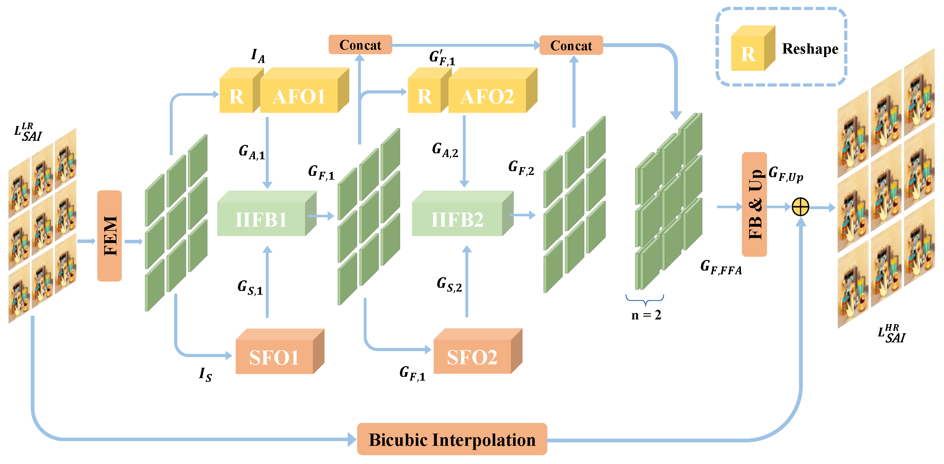
3.2. Network Architecture

Our LF-FANet mainly consists of three parts: a feature extraction module ($f_{FEM}$), a feature fusion and allocation module ($f_{FFA}$) and a feature blending and upsampling module ($f_{\mathrm{F}\mathrm{B}\&\mathrm{U}\mathrm{P}}$). These three parts are shown in Figure 2. The feature extraction module is used to obtain the shallow features from each SAI. Then, we design the second part for feature fusion and allocation, which contains two different operators (AFO, SFO), and an interaction information fusion block (IIFB). This part adopts a fusion and allocation strategy to interact with high-dimensional information (angular and spatial dimensions) and distribute the information for further angular-and-spatial deep representation. Finally, the feature blending and upsampling modules are utilized to generate more compact representations and reconstruct residual maps. Specifically, the LR SAIs ($L_{SAI}^{LR}$) as input are fed into a $1\times 1$ convolution to generate initial features. These features are processed by two cascaded DASPPs; this is introduced in Section 3.2.1. Processed by our $f_{FEM}$, the hierarchical features ($I_S$) of all SAIs are generated. That is,

$$I_S=f_{FEM}\left(L_{SAI}^{LR}\right),$$

(1)

where $I_S\in {\mathbb{R}}^{N\times C\times H\times W}$ represents the hierarchical features, $N=U\times V$ denotes the number of SAIs, and the feature depth is C. Then, $I_S$ is directly fed into the SFO. Meanwhile, we reshape features $I_S$ to $I_A\in {\mathbb{R}}^{C\times N\times H\times W}$ and feed $I_A$ into the AFO. That is,

$$\begin{array}{cc}\hfill G_{A,k}& =f_{AFO,k}\left(I_A\right),\hfill \\ \hfill G_{S,k}& =f_{SFO,k}\left(I_S\right),\hfill \end{array}$$

(2)

where $f_{AFO,k}$ and $f_{SFO,k}$ are two operators for angular and spatial information extraction. $G_{A,k}$ and $G_{S,k}$ are the output of AFO and SFO. Following our fusion strategy, these two features are fully fused by IIFB, which can be expressed as,

$$G_{F,k}=f_{IIFB,k}\left(G_{A,k},G_{S,k}\right),$$

(3)

where $G_{F,k}$ represents the fusion feature with informative angular and spatial information. Then, the allocation operation is performed. $G_{F,k}$ is fed into the second $f_{AFO,2}$ and $f_{SFO,2}$, respectively. In our network, we repeat our strategy twice, which can obtain two hierarchical fusion features $G_{F,1}$ and $G_{F,2}$. We concatenate these features as the output of $f_{FFA}$, which can be expressed as,

$$G_{F,FFA}=f_{Cat}\left(G_{F,1},G_{F,2}\right),$$

(4)

where $f_{Cat}$ denotes the concatenation operation, and $G_{F,FFA}$ is the output feature of $f_{FFA}$. Finally, the $G_{F,FFA}$ is fed into a feature blending and upsampling module (FB & UP) to generate an HR residual map ($G_{F,\mathrm{F}\mathrm{B}\&\mathrm{U}\mathrm{P}}$), which adds a bicubic interpolation to generate the final SR images. The process of reconstructing all SR images can be simply expressed as,

$$\begin{array}{cc}\hfill G_{F,\mathrm{F}\mathrm{B}\&\mathrm{U}\mathrm{P}}& =f_{\mathrm{F}\mathrm{B}\&\mathrm{U}\mathrm{P}}\left(G_{F,FFA}\right),\hfill \\ \hfill L_{SAI}^{HR}& =G_{F,\mathrm{F}\mathrm{B}\&\mathrm{U}\mathrm{P}}+f_{Cubic}\left(L_{SAI}^{LR}\right),\hfill \end{array}$$

(5)

where $f_{Cubic}$ is the bicubic interpolation operation, and $L_{SAI}^{HR}$ is the HR SAIs.

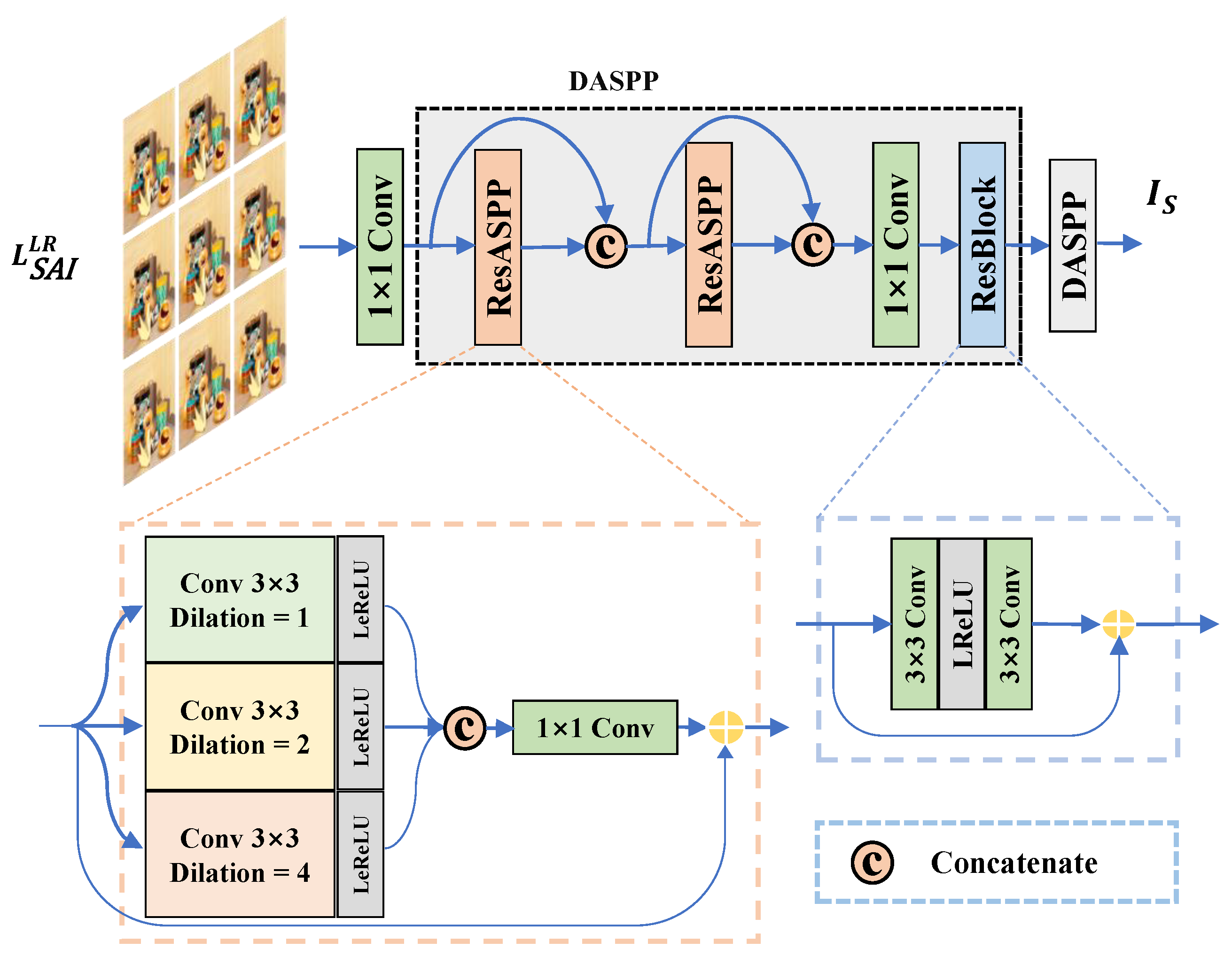
3.2.1. Feature Extraction Module (FEM)

Due to the intrinsic characteristics of LF, an amount of redundant information exists among different views. Therefore, it is meaningful to deepen the network to effectively extract discriminative features in each view. Meanwhile, each view contains rich contextual information, which can be captured by enlarging the receptive field. This information is helpful for reconstructing HR LF images with more details. Our FEM is mainly to extract features for the part of feature fusion and allocation. Inspired by the work in Deeplab and deformable convolution [16,32], we designed a DASPP block to enlarge the receptive field and extract hierarchical features for each view, as shown in Figure 3. This block consists of two cascaded residual atrous spatial pyramid poolings (ResASPP) with dense skip connections. Due to this connection, our DASPP can preserve hierarchical features while providing dense representative information to the utmost extent. Compared with the extraction by a residual block, the superior effectiveness of our DASPP is demonstrated in Section 4.4.

The details of our FEM are shown in Figure 3, it is mainly composed of two components: the DASPP and the residual block (ResBlock). Each SAI is first put into a $1\times 1$ convolution to extract initial features. These features are fed into two DASPPs with identical structures. Each DASPP has two ResASPP blocks, which are constructed by three dilated convolutions with different dilation rates (1, 2, 4). These dilated convolutions, following a Leaky ReLU, are concatenated to obtain hierarchical features, which are concatenated with the initial features to feed into another ResASPP block. The input and output features of this ResASPP are concatenated to feed into a $1\times 1$ convolution to adjust the channel depth. The ResBlock consists of two $3\times 3$ convolutions and a Leaky ReLU activation. In summary, the deep and hierarchical features ($I_S$) of each SAI are extracted by using our FEM.

3.2.2. Feature Fusion and Allocation Module (FFAM)

For the high-dimensionality characteristic of LF, it is challenging to effectively extract deep representation from high dimensions. Meanwhile, fully fusing angular and spatial information among all LFs still needs to be explored, which is beneficial for preserving LF structural consistency. Many approaches concatenate the information from these two dimensions together, seriously affecting the performance of the network. To reduce the impact of this problem and improve the SR performance, we especially designed two generic operators for 4D LF to achieve angular-wise and spatial-wise feature fusion. These two operators are divided into dual branches to deal with. In each branch, AFO and SFO can effectively integrate angular-wise and spatial-wise features, respectively. Then, we propose a fusion and allocation strategy to achieve the angular and spatial information interaction while achieving the parallax structure of LF. The core component of this strategy is IIFB. Following our strategy, the output features of IIFB are individually fed into the next two operators, which can further achieve the process of feature allocation.

In our FFAM, the hierarchical features ($I_S$) are fed into two branches to incorporate angular correlations in angular subspace and supplement context information in spatial subspace, as depicted in Figure 2. Note that, for the top branch, we perform a reshape operation to obtain the input feature $I_A\in {\mathbb{R}}^{C\times N\times H\times W}$. Comparing with the $I_S\in {\mathbb{R}}^{N\times C\times H\times W}$, we only swap the first two dimensions. The slice of each C dimension represents all the angular information (${\mathbb{R}}^{N\times H\times W}$) from all SAIs. For the bottom branch, we can obtain the spatial information (${\mathbb{R}}^{C\times H\times W}$) containing all the channels of each SAI.

3.2.3. Angular Fusion Operator (AFO)

The objective of this operator is to effectively exploit the angular correlation. Inspired by the structure of the encoder and decoder, the main structure of AFO is UpConv and DownConv to execute upscaling and downscaling operations, as shown in Figure 4. Specifically, it can map the angular-wise features from all SAIs to high-dimension space for interaction by the encoder and decoder structure. Moreover, ResASPP blocks make the high-dimension and low-dimension features with different receptive fields, which are beneficial for exploiting the angular correlation.

Taking the first AFO as an example, the reshaped feature $I_A\in {\mathbb{R}}^{C\times N\times H\times W}$ is first fed into a cascaded encoder and decoder structure with a skip connection, which consists of two ResASPP blocks—an UpConv and a DownConv. These two ResASPP blocks are respectively inserted in front of the UpConv and DownConv. The output feature $I_{A,Down}$ of DownConv is fed into a $3\times 3$ convolution and a Leaky ReLU. Then, the output is concatenated with $I_A$ to keep hierarchical characteristics. A $1\times 1$ convolution and a Leaky ReLU are used for angular depth reduction. This process can be specifically expressed as,

$$\begin{array}{cc}\hfill I_{A,Down}& =\left[f_{DownConv}\circ f_{ResASPP}\circ f_{UpConv}\circ f_{ResASPP}\right]\left(I_A\right),\hfill \\ \hfill G_{A,1}& =\left[f_{{Conv}_2}\circ f_{Cat}\left(·,I_A\right)\circ f_{{Conv}_1}\right]\left(I_{A,Down}\right),\hfill \end{array}$$

(6)

where $f_{ResASPP}$ represents the ResASPP block, $f_{UpConv}$ and $f_{DownConv}$ represent two types of convolutions, which have different parameters for different up-sampling scales; $f_{{Conv}_1}$ and $f_{{Conv}_2}$ represent the $3\times 3$ convolution and the $1\times 1$ convolution, respectively, and $f_{Cat}$ denotes the concatenate operation. Due to the input $I_A\in {\mathbb{R}}^{C\times N\times H\times W}$, the number of channels of these modules and convolutions is N. As shown in Figure 2, there are two AFOs used in our network. The other AFO can be simply expressed as

$$G_{A,2}=f_{AFO,2}\left(G_{F,1}^{\prime }\right),$$

(7)

where $f_{AFO,2}$ is the second AFO, and ${G^{\prime }}_{F,1}$ and $G_{A,2}$ represent the input and output features, respectively.

3.2.4. Spatial Fusion Operator (SFO)

For the spatial-wise branch, this operator has a similar structure to AFO, which also has an encoder and decoder structure. As shown in Figure 5, we take the first SFO as an example. The features $I_S\in {\mathbb{R}}^{N\times C\times H\times W}$ from each SAI are first fed into a ResASPP. Then, UpConv is utilized to map the spatial information from the low dimension to the high dimension. After the second ResASPP, the DownConv converts the high-dimension features to low-dimension features $I_{S,Down}$. The low-dimension features of the SFO can be expressed as

$$I_{S,Down}=\left[f_{DownConv}^{\prime }\circ f_{ResASPP}^{\prime }\circ f_{UpConv}^{\prime }\circ f_{ResASPP}^{\prime }\right]\left(I_S\right),$$

(8)

where $f_{ResASPP}^{\prime }$ represents the ResASPP block, $f_{UpConv}^{\prime }$ and $f_{DownConv}^{\prime }$ represent two types of convolutions, which have different parameters for different up-sampling scales. The number of channels of $f_{ResASPP}^{\prime }$, $f_{UpConv}^{\prime }$ and $f_{DownConv}^{\prime }$ is C. The output feature $I_{S,Down}$ is closely fed into a $3\times 3$ convolution and a Leaky ReLU, which perform the concatenate operation with $I_S$ to preserve the initial information. After that, a $1\times 1$ convolution and a Leaky ReLU are used to reduce the channel depth.

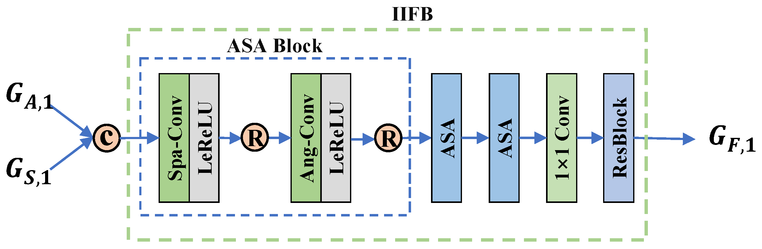
3.2.5. Interaction Information Fusion Block (IIFB)

Most existing methods of LF image SR lack the consideration of the vinformation fusion of the angular and spatial dimensions, which seriously destroys the parallax structure of LF. Although 4D convolution can be directly utilized to deal with this problem, it causes a significant increase in computation. Inspired by the methods of Yeung et al. [33] and Jin et al. [14], we designed our IIFB, which mainly consists of three alternative spatial-angular convolutions (ASA). Compared with the 4D convolutions, this convolution not only reduces computational resources but also fully explores the angular and spatial information. In short, our IIFB can achieve complementary information fusion from all SAIs as well as discriminative information fusion among all SAIs.

As shown in Figure 6, we take the first IIFB as an example. The input of IIFB consists of two parts—the output of AFO ($G_{A,1}$) and the output of SFO ($G_{S,1}$). We first concatenate $G_{A,1}$ and $G_{S,1}$ in the channel dimension. These features are fed into three cascaded ASA blocks. Each ASA contains the convolution of Spa-Conv and Ang-Conv, the kernel size of which is $3\times 3$. Then, a $1\times 1$ convolution and a ResBlock are used to further extract the depth feature representation. Following our fusion and allocation strategy, we distribute the output ($G_{F,1}$) of IIFB into the next AFO and SFO.

In summary, many previous LF image SR methods treat the 4D LF as a unity, which affects representational capacities. Due to the independent properties of angular and spatial information, we propose AFO, SFO and IIFB to extract and fuse the spatial-angular information. The main structure of AFO and SFO refers to the encoder and decoder method, which can better mine the mapping relationship between LR images and HR images. Due to supervised learning, the differences are gradually narrowed between the output features of UpConv and the final features of HR. Meanwhile, the function of DownConv is to reduce computation with low-dimension features. Moreover, our operators are not focused on local information caused by the kernel size of convolution. The AFO can capture global channel information from different views, and the SFO can fuse multi-view spatial information. After this, we apply IIFB to achieve information fusion. Meanwhile, compared with the similar mechanisms (angular feature extractor and spatial feature extractor) in LF-InterNet [15], our IIFB does not concatenate spatial and angular information directly, which can better preserve the geometry structure, which is better for the performance of LF. Our LF-FANet can not only preserve the parallax structure of LF but also supplement complementary information from different SAIs.

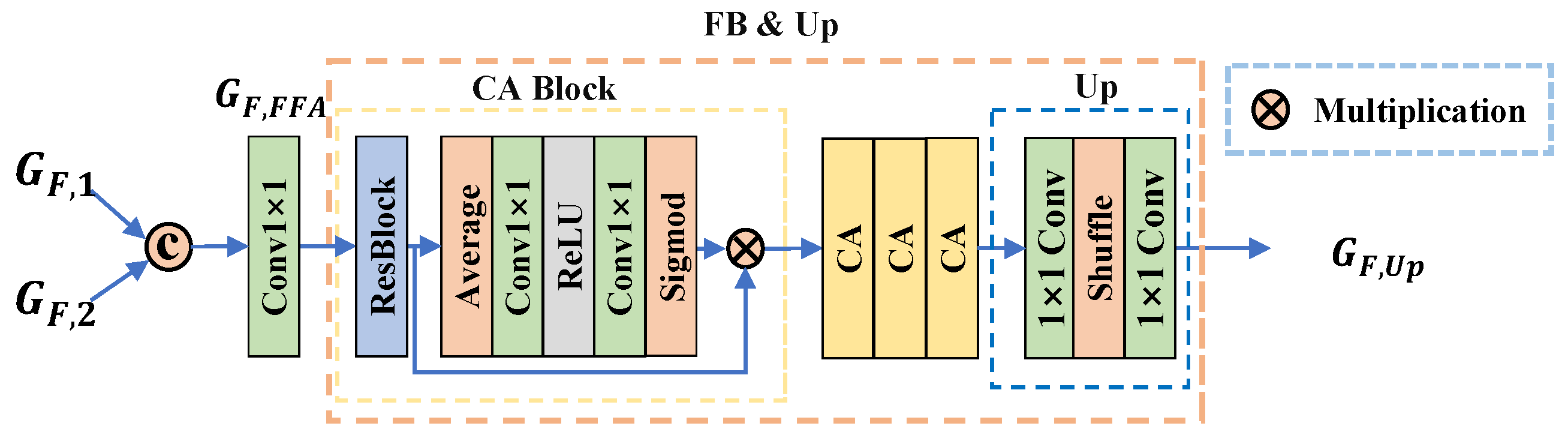
3.2.6. Feature Blending and Upsampling Module (FB & UP)

Combining the hierarchical features is beneficial for constructing the HR residual map. However, directly concatenating these features cannot adaptively adjust the contributions of the hierarchical features. Following Wang et al. [16], we concatenate each output $G_{F,1}$ and $G_{F,2}$ of IIFB along the channel dimension, and input it into the FB & UP module to obtain the final residual map $G_{F,\mathrm{F}\mathrm{B}\&\mathrm{U}\mathrm{P}}$. Note that the output $G_{F,1}$ and $G_{F,2}$ are gradually generated containing hierarchical information, which has a different importance for $G_{F,\mathrm{F}\mathrm{B}\&\mathrm{U}\mathrm{P}}$. Therefore, we introduce the channel attention module [34] to dynamically adapt the hierarchical features and distillate the valid information.

The architecture of our FB & UP module is illustrated in Figure 7. $G_{F,FFA}$ is the hierarchical features, which is the input of FB & UP module. In this module, we cascade four channel attention (CA) blocks and an Up block. Note that the CA block plays a key role in the feature blending, which is formed by a ResBlock cascaded with a CA block. Specifically, Average is a global average pooling operation, which is used to squeeze the spatial information of each channel. Then, we generate an attention map by utilizing two $1\times 1$ convolutions and a ReLU layer. The objective of the first convolution is to compress the channel numbers, and the second convolution aims to recover the original channel numbers. The reduction ratio and expansion ratio for these two convolutions are set to $0.5\times$ and $2\times$, respectively. To refine the features across all channels, this attention map is processed by a sigmoid function. After processing by the other three CA blocks, feature blending can be achieved on the hierarchical features. The Up block is composed of a $1\times 1$ convolution, a Shuffle layer and another $1\times 1$ convolution. The output $G_{F,\mathrm{F}\mathrm{B}\&\mathrm{U}\mathrm{P}}$ has only one channel number with the enlarged SAI size. The effectiveness of FB is demonstrated in Section 4.

3.3. Loss Function

Our LF-FANet is an end-to-end network to achieve all LF image reconstruction. To train our network, the L1 loss function is used to minimize the absolution error between the reconstructed SAIs ($L_{SAI}^{HR}$) and its ground-truth ($L_{SAI}^{GT}$). $L_{SAI}^{HR}$ is generated by LF-FANet and is related to $L_{SAI}^{LR}$. There is a total of N training pairs for the training process,

$$\mathcal{L}=\frac{1}{N}\sum _{n=1}^N{∥L_{SAI}^{HR}-L_{SAI}^{GT}∥}_{L1}.$$

(9)

4. Experiments

In this section, we discuss the details of our datasets and evaluation metrics. Then, we present the settings and implementation details of our LF-FANet. After that, we compare our LF-FANet with several state-of-the-art SISR and LF image SR methods. Finally, we present the ablation studies to investigate the performance of each component of our network.

4.1. Datasets and Evaluation Metrics

To validate the generalization performance of our LF-FANet, five rich scenarios of LF datasets were used in our experiments, divided into two types. As listed in

Table 1. Public LF datasets used in our experiments.

Datasets	Training	Test	LF Disparity	Type
HCInew [35]	20	4	[−4, 4]	Synthetic
HCIold [36]	10	2	[−3, 3]	Synthetic
EPFL [37]	70	10	[−1, 1]	Real-world
INRIA [38]	35	5	[−1, 1]	Real-world
STFgantry [39]	9	2	[−7, 7]	Real-world
Total	144	23

, HCInew [35] and HCIold [36] are synthetic images. EPFL [37] and INRIA [38] were captured by Lytro Illum cameras from real-world scenes, and STFgantry [39] was captured by cameras on a gantry. For robust reference, there was a total of 144 LF images trained together, which were randomly selected from six datasets. The rest of the LF images in each dataset were used for testing. Note that each dataset has various LF disparity ranges for different scenes. Specifically, STFgantry has the largest LF disparity. EPFL and INRIA have the same disparity. All these datasets have an angular resolution of $9\times 9$. The input for training and testing was generated by using the bicubic downsampling operation. For performance evaluation, Peak Signal-to-Noise Ratio (PSNR) and structural similarity (SSIM) were used as quantitative metrics. The higher value of these two metrics denotes a better LF reconstruction performance. In our experiments, PSNR and SSIM were used on the Y-channel of LF images to evaluate all the different methods. The perceptual metric named LPIPS [40] was used in this paper, which can evaluate the performance of different methods on RGB images.

4.2. Settings and Implementation Details

Here, we list the more specific settings and implementation details of our network. The channel depth of convolution (C) was set to 32. We had 2 AIOs, 2 SIOs and 2 IIFBs. The outputs of all IIFBs were concatenated and, in total, had $32\times 2$ filters for the convolution layer in FB. N was 25 for the $5\times 5$ angular resolution of the LF input, which had a $32\times 32$ spatial resolution for each input. The upsampling scales $\alpha$ were $2\times$ and $4\times$, respectively. To augment the training data, we randomly processed the data by flipping and rotating with a degree of 90. Our network adopted the L1 Loss function. The Adam optimizer was used with ${\beta }_1=0.9$ and ${\beta }_2=0.999$. The initial learning rate was $2\times {10}^{-4}$, which decreased to half after 15 epochs. The maximum epoch was equal to 98. The batch size was set to 38. Our network was based on the PyTorch framework. This code was run on a PC with Ubuntu 20.04 OS, which had an NVIDIA QUADRO RTX 8000 GPU and two CPUs of Intel(R) Xeon(R) Silver 4216.

4.3. Comparisons with State-of-the-Art Methods

To evaluate the effectiveness of our LF-FANet, we compared our method with two categories of SR methods. One category was the SISR methods, including two algorithms, the other was the LF image SR methods including eight LF image SR algorithms. Specifically, they were VDSR [10], EDSR [11], LFSSR [33], resLF [13], LF-ATO [14], LF-InterNet [15], LF-DFNet [16], MEG-Net [17], DPT [30] and LF-IINet [20]. Note that all learning-based methods were retained in the same training datasets to keep a fair comparison. Moreover, bicubic interpolation was used as a baseline in our paper.

4.3.1. Quantitative Results

The quantitative results are shown in

Table 2. PSNR/SSIM/LPIPS values achieved by different methods for $2\times$ and $4\times$ SR, the best results are in bold and the second best results are underlined.

Methods	Scale	Datasets					Average
		EPFL	HCInew	HCIold	INRIA	STFgantry
Bicubic	$2\times$	29.50/0.935/0.198	31.69/0.934/0.222	37.46/0.978/0.115	31.10/0.956/0.200	30.82/0.947/0.156	32.11/0.950/0.178
VDSR [10]		32.64/0.960/0.092	34.45/0.957/0.122	40.75/0.987/0.050	34.56/0.975/0.093	35.59/0.979/0.034	35.60/0.972/0.078
EDSR [11]		33.05/0.963/0.077	34.83/0.959/0.111	41.00/0.987/0.047	34.88/0.976/0.080	36.26/0.982/0.022	36.00/0.973/0.067
LFSSR [33]		32.84/0.969/0.050	35.58/0.968/0.069	42.05/0.991/0.027	34.68/0.980/0.066	35.86/0.984/0.032	36.20/0.978/0.049
resLF [13]		33.46/0.970/0.044	36.40/0.972/0.039	43.09/0.993/0.018	35.25/0.980/0.057	37.83/0.989/0.017	37.21/0.981/0.035
LF-ATO [14]		34.22/0.975/0.041	37.13/0.976/0.040	44.03/0.994/0.017	36.16/0.984/0.056	39.20/0.992/0.011	38.15/0.984/0.033
LF-InterNet [15]		34.14/0.975/0.040	37.28/0.977/0.043	44.45/0.995/0.015	35.80/0.985/0.054	38.72/0.991/0.035	38.08/0.985/0.037
LF-DFNet [16]		34.44/0.976/0.045	37.44/0.979/0.048	44.23/0.994/0.020	36.36/0.984/0.058	39.61/0.994/0.015	38.42/0.985/0.037
MEG-Net [17]		34.30/0.977/0.048	37.42/0.978/0.063	44.08/0.994/0.023	36.09/0.985/0.061	38.77/0.991/0.028	38.13/0.985/0.044
DPT [30]		34.48/0.976/0.045	37.35/0.977/0.046	44.31/0.994/0.019	36.40/0.984/0.059	39.52/0.993/0.015	38.41/0.985/0.037
LF-IINet [20]		34.68/0.977/0.038	37.74/0.978/0.033	44.84/0.995/0.014	36.57/0.985/0.053	39.86/0.993/0.010	38.74/0.986/0.030
DistgSSR [31]		34.78/0.978/0.035	37.95/0.980/0.030	44.92/0.995/0.014	36.58/0.986/0.051	40.27/0.994/0.009	38.90/0.987/0.028
Ours		34.81/0.979/0.034	37.93/0.979/0.030	44.90/0.995/0.014	36.59/0.986/0.050	40.30/0.994/0.008	38.91/0.987/0.027
Bicubic	$4\times$	25.26/0.832/0.435	27.71/0.852/0.464	32.58/0.934/0.339	26.95/0.887/0.412	26.09/0.845/0.432	27.72/0.870/0.416
VDSR [10]		27.22/0.876/0.287	29.24/0.881/0.325	34.72/0.951/0.204	29.14/0.920/0.278	28.40/0.898/0.198	29.74/0.905/0.258
EDSR [11]		27.85/0.885/0.270	29.54/0.886/0.313	35.09/0.953/0.197	29.72/0.926/0.268	28.70/0.906/0.175	30.18/0.911/0.245
LFSSR [33]		28.13/0.904/0.246	30.38/0.908/0.281	36.26/0.967/0.148	30.15/0.942/0.245	29.64/0.931/0.180	30.91/0.931/0.220
resLF [13]		28.17/0.902/0.236	30.61/0.909/0.261	36.59/0.968/0.136	30.25/0.940/0.233	30.05/0.936/0.141	31.13/0.931/0.202
LF-ATO [14]		28.74/0.913/0.222	30.97/0.915/0.256	37.01/0.970/0.135	30.88/0.949/0.220	30.85/0.945/0.116	31.69/0.938/0.190
LF-InterNet [15]		28.58/0.913/0.227	30.89/0.915/0.258	36.95/0.971/0.131	30.58/0.948/0.227	30.32/0.940/0.133	31.47/0.937/0.195
LF-DFNet [16]		28.53/0.906/0.225	30.66/0.900/0.269	36.58/0.965/0.134	30.55/0.941/0.226	29.87/0.927/0.159	31.32/0.928/0.203
MEG-Net [17]		28.75/0.902/0.239	31.10/0.907/0.278	37.29/0.9663.144	30.67/0.940/0.239	30.77/0.930/0.179	31.72/0.929/0.216
DPT [30]		28.93/0.917/0.241	31.19/0.919/0.273	37.39/0.972/0.145	30.96/0.950/0.236	31.14/0.949/0.157	31.92/0.941/0.210
LF-IINet [20]		29.04/0.919/0.215	31.36/0.921/0.245	37.44/0.973/0.123	31.03/0.952/0.216	31.21/0.950/0.125	32.02/0.943/0.185
DistgSSR [31]		28.98/0.919/0.231	31.38/0.922/0.244	37.38/0.971/0.134	30.99/0.952/0.227	31.63/0.954/0.118	32.07/0.944/0.191
Ours		29.14/0.920/0.213	31.41/0.923/0.235	37.50/0.973/0.112	31.04/0.952/0.213	31.68/0.954/0.109	32.15/0.944/0.176

. The metrics of PSNR and SSIM were employed to evaluate the SR accuracy on five testing datasets. Moreover, the metrics of LPIPS were used to evaluate the difference between SR image and the ground-truth image. The best results and the second-best results are shown in bold and underlined, respectively. Meanwhile, the average values of PSNR and SSIM are presented to show the generalization of different complex scenes. It can be noticed that our LF-FANet achieved state-of-the-art results on both the $2\times$ and $4\times$ average values. For these testing datasets, our method achieved the highest PSNR and SSIM scores for the $4\times$ SR. For $2\times$ and $4\times$ SR, our method was slightly inferior to DistgSSR on HCIold and HCInew. Specifically, compared with the SISR methods (VDSR), we achieved 3.31 dB (0.015) higher in terms of the average PSNR (SSIM) for $2\times$ SR. That is because SISR methods ignore the supplement of angular information from other views, which hinders further improvements in SR. Compared with the current learning-based method (LF-DFNet), our method obtained superior results on EPFL, having a 0.61 dB (0.014) higher PSNR (SSIM) for $4\times$ SR. Compared with DPT, LF-FANet achieved 0.50 dB and 0.23 dB higher in terms of average PSNR for $2\times$ SR and $4\times$ SR, respectively. Moreover, both our LF-FANet and LF-IINet had the smallest values of LPIPS, which indicates that the SR images from these two methods are more similar to ground-truth images. Our LF-FANet achieved a state-of-the-art performance by treating the spatial and angular domains equally and incorporating the information of these two domains.

Interestingly, it can be observed that our LF-FANet achieved a better result on the large disparity dataset (STFgantry), whose scenes were captured by a moving camera mounted on a gantry. This is attributed mainly to our fusion and allocation strategy. In the fusion stage, the proposed IIFB can interact and fuse informative information from spatial and angular domains, which is beneficial for preserving the parallax structure of LF views. In the allocation stage, the output of the fusion stage is distributed to the next AFO and SFO. These two operators can better cover the influence of large disparities with multi-scale receptive fields and equally deal with angular and spatial information.

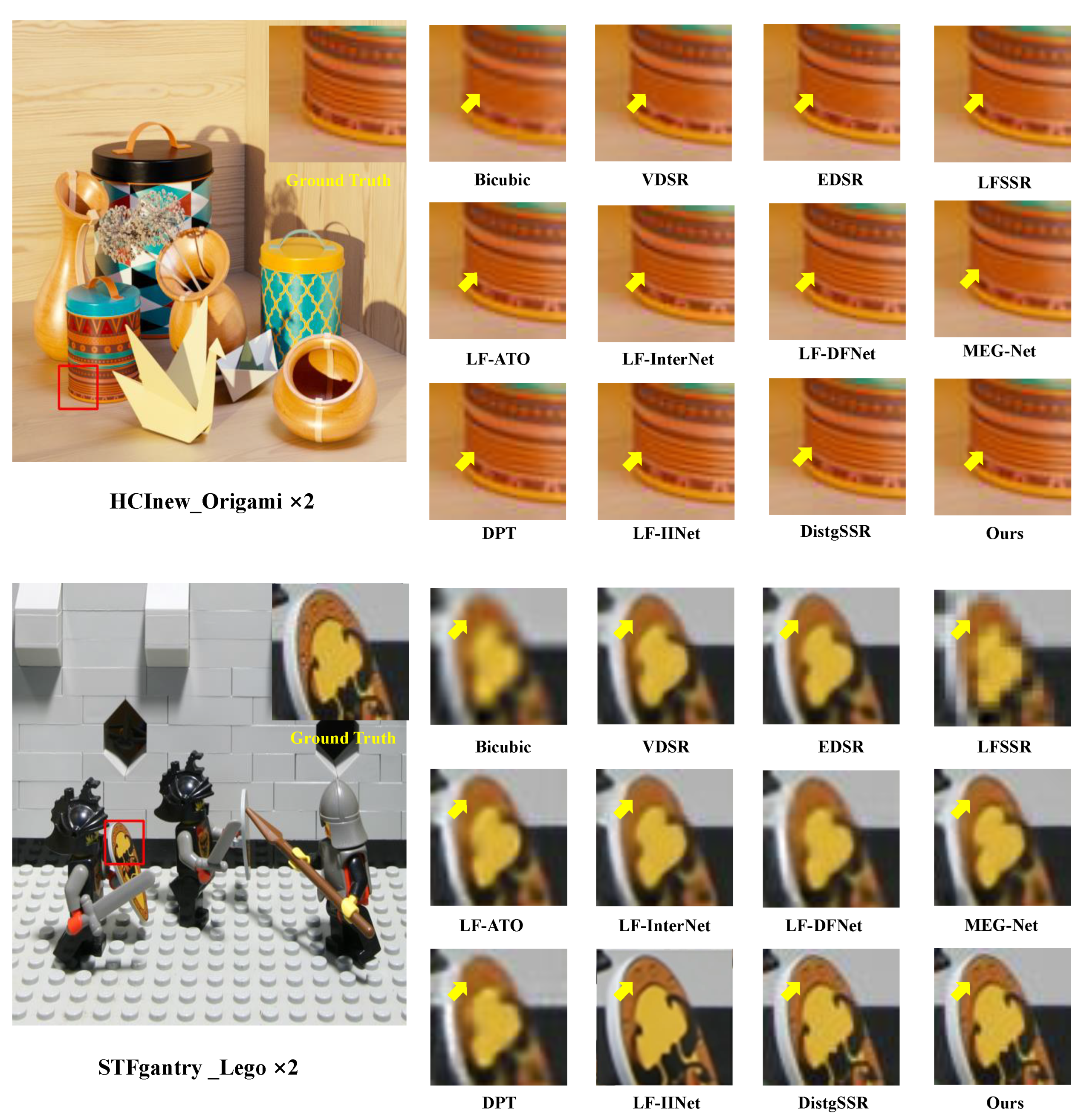
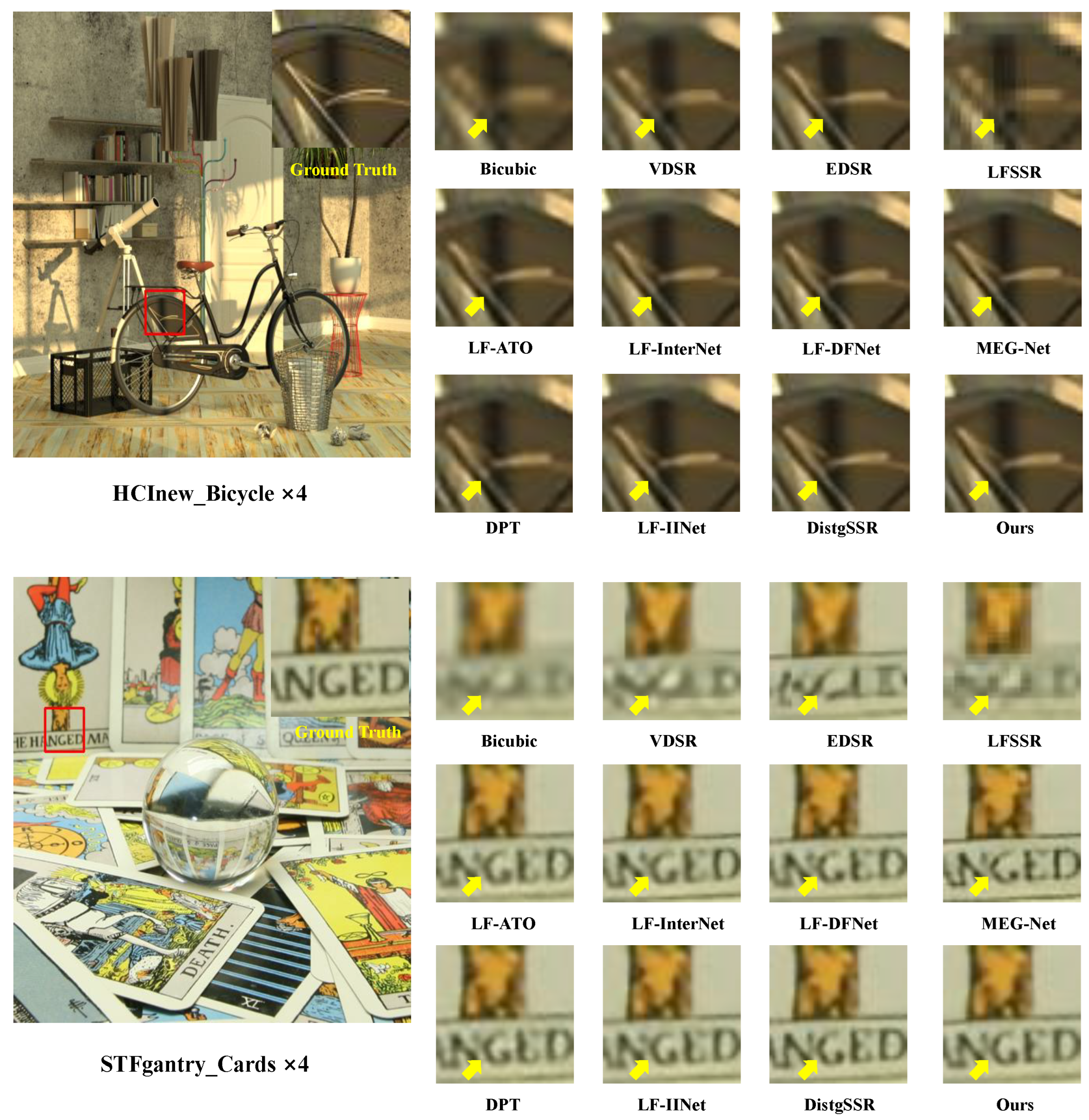
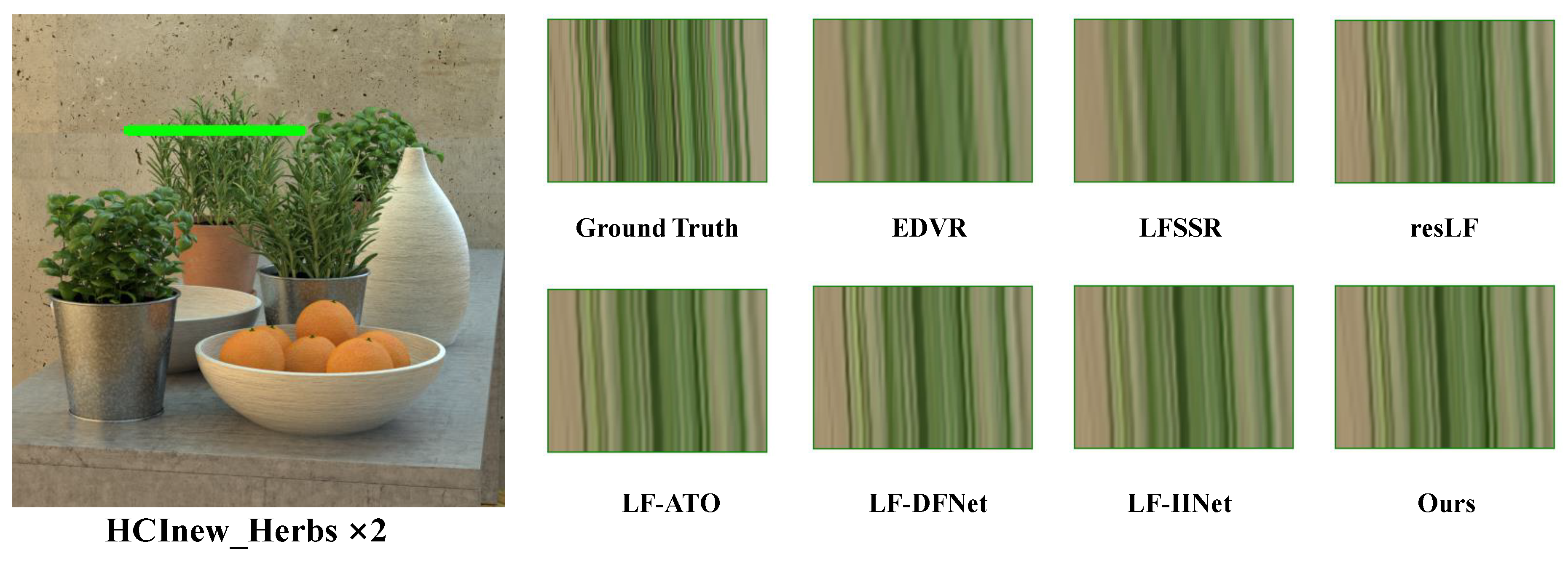
4.3.2. Qualitative Results

The qualitative results for $2\times$ and $4\times$ SR are shown in Figure 8 and Figure 9, respectively. We zoom in on the visualization of the center view of different methods. Compared with other methods, our method can produce high-quality HR LF images with more details and fewer artifacts, especially for $4\times$ SR. Four typical complex scenes were used to present the qualitative results, which were HCInew_Origami, STFgantry_Lego, HCInew_Bicycle, and STFgantry_Cards. As shown in Figure 8, for $2\times$ SR, the images generated by SISR methods (VDSR and EDSR) are blurry on pattern regions, which are better than those of the bicubic interpolation method. Note that the results achieved by the LFSSR method have pixel tiles, especially on the scene of STFgantry_Lego. In contrast, our LF-FANet can produce images very close to the ground truth. Compared with $2\times$ SR, $4\times$ SR is more challenging, because the reconstruction contains less information. As shown in Figure 9, in the results of VDSR, EDSR, and LFSSR, it is difficult to recognize the letters in scene STFgantry_Cards, which is very challenging due to the complex structures and occlusions. As shown in Figure 10, there is another visual example, which is the distance map between the $4\times$ SR image and the ground-truth map. For the zoom area with a red rectangle, it can be observed that our method is close to ground-truth LF. Compared with our method, the results of the rest of LF image SR methods present a degree of artifacts and ambiguities.

As shown in Figure 11, we also present the EPIs, which can reflect the quality of the parallax structure of LF images. In scene HCInew_Herbs for $4\times$ SR, the blurry EPIs of EDVR and LFSSR can be observed, indicating that both are not able to keep the parallax consistency. Although the EPIs of resLF, LF-ATO, LF-DFNet, LF-IINet and our LF-FANet methods are similar to the ground truth EPI, our method has the least blurry artefacts and the clearest textures in EPIs. In summary, our method can not only reconstruct high-quality LF images but also keep the structure of LF parallax.

4.3.3. Parameters and FLOP

In

Table 3. Comparative results in terms of the number of parameters, FLOPs, and average PSNR/SSIM on testing sets for $4\times$ LF image SR methods. The best results are in bold.

Ang	Scale	Params. (M)	FLOPs (G)	Avg. PSNR/SSIM
EDSR [11]	$4\times$	38.89	1016.59	30.18/0.911
LFSSR [33]		1.77	113.76	31.23/0.935
LF-ATO [14]		1.36	597.66	31.69/0.938
LF-DFNet [16]		3.94	57.22	31.32/0.928
DPT [30]		3.78	58.64	31.92/0.941
LF-FANet (Ours)		3.38	257.38	32.15/0.944

, we compare the number of parameters (Param.), FLOPs and the average of PSNR and SSIM (Avg. PSNR/SSIM) between our LF-FANet and other methods of testing datasets for $4\times$ upscaling. Our method achieves the highest scores of average PSNR and SSIM, shown in boldface. Although LF-ATO has the smallest number of parameters, its computational FLOPs with a $5\times 5\times 32\times 32$ LF image are very high. This is because the structure of LF-ATO is designed as an all-to-one model, which reconstructs all views one by one. Compared with LF-ATO, our method has a slightly higher number of parameters but consumes lower FLOPs. Furthermore, our LF-FANet has fewer parameters and achieves a better performance than other all-to-all methods, such as DPT, LF-DFNet, etc. In summary, our method has good standing, not only in terms of the performance of the model but also in terms of the scores of PSNR and SSIM.

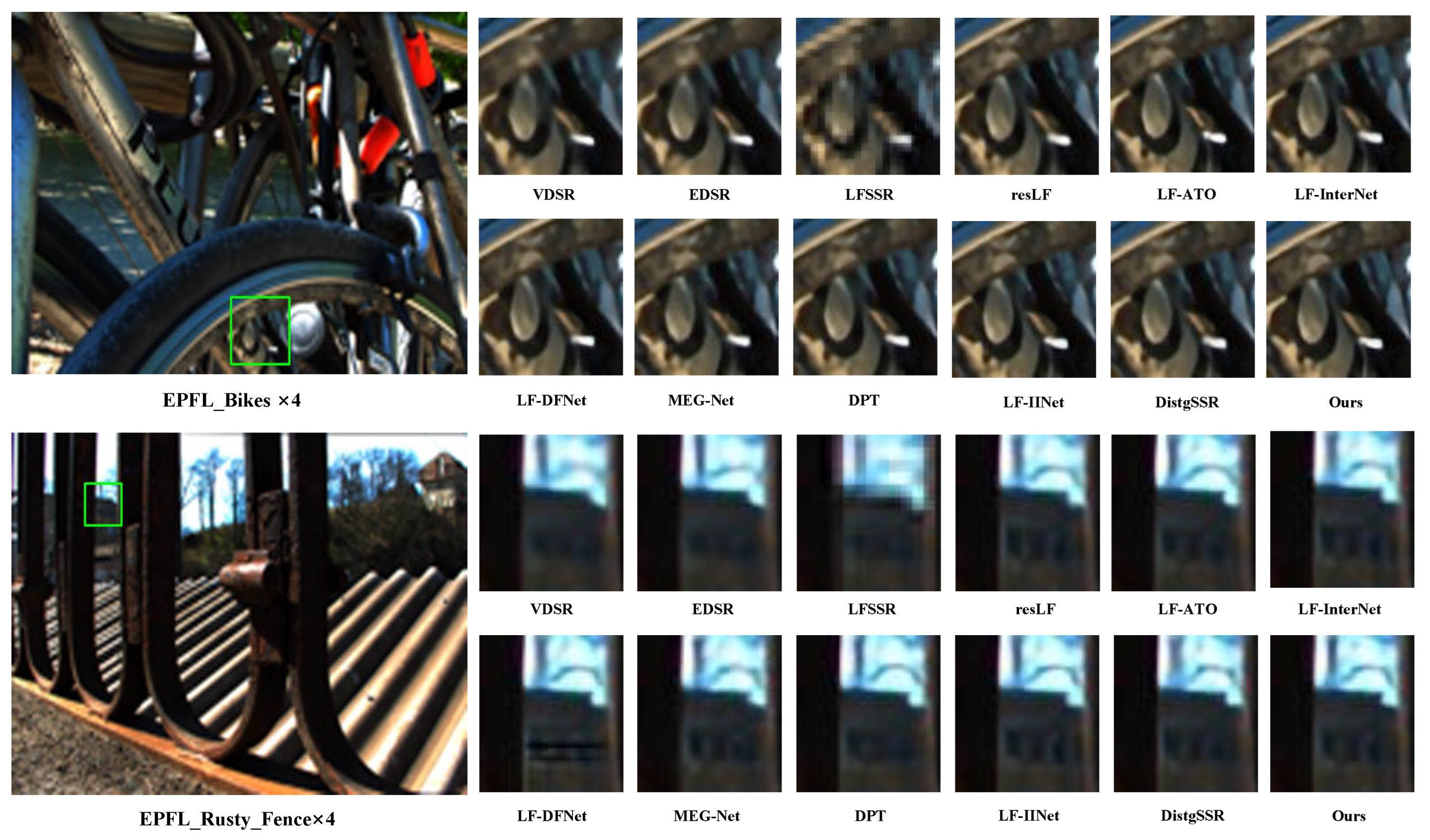
4.3.4. Performance on Real-World LF Images

We compared our method with other SISR methods (VDSR and EDSR) and LF image SR methods (LFSSR, resLF, LF-ATO, LF-InterNet, MEG-Net, DPT, LF-IINet and DistgSSR) on real-world LF images, which were provided by the EPFL dataset [37]. Since ground truth HR images were not available, we directly compared the performance of reconstruction using these real-world images as input. As shown in Figure 12, our LF-FANet can reconstruct an HR image that is less blurry than VDSR and EDSR, and with fewer artifacts than LFSSR. In summary, our method can be applied to LF cameras to generate high-quality LF images.

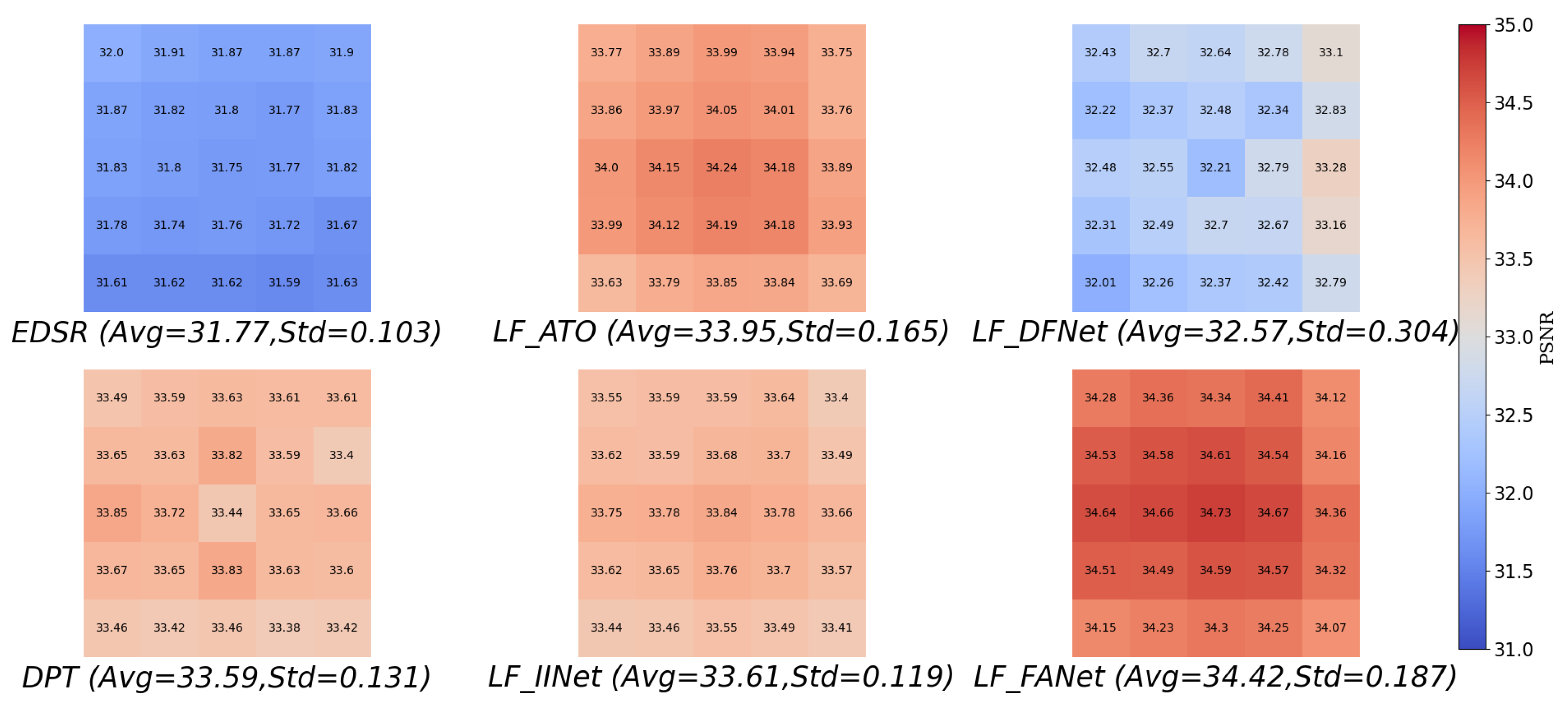
4.3.5. Performance of Different Perspectives

In order to exhibit the SR performance of different perspectives, we compared the reconstruction quality of each view in an LF scene with several state-of-the-art methods. As shown in Figure 13, we present the value of PSNR for $5\times 5$ perspectives of the INIRA_Hublais scene from INRIA at $4\times$ SR. The average PSNR of all perspectives and the standard deviation of all the perspectives were used to evaluate the performance. It can be observed that EDSR has the lowest average PSNR and lowest Std. That is because EDVR is the SISR method, which just super resolves each view that lacks the angular correlations. Compared with other LF image SR methods, our LF-FANet achieved the highest average PSNR and a lower Std, which demonstrates that our method can not only reconstruct high-quality images but also keep a strong consistency among all views.

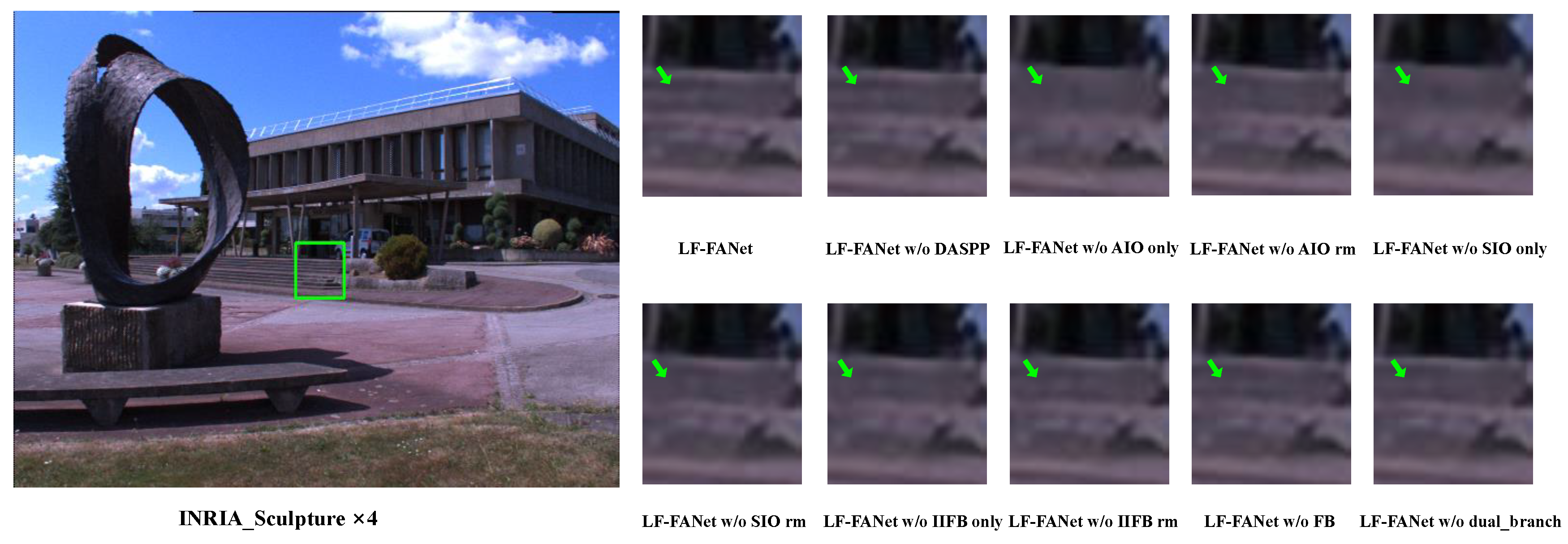
4.4. Ablation Study for Different Components of LF-FANet

In this subsection, we implemented several ablation experiments to validate the effectiveness of different components of our LF-FANet, including the DASPP module, the SFO, the AFO, the IIFB, the structure of dual branches, and the FB. Meanwhile, the visual results of our LF-FANet with different variants are shown in Figure 14. It can be observed that all variants of our network have a degradation in performance, pointed out by the green arrows. In

Table 4. PSNR/SSIM values achieved by LF-FANet and its variants for $4\times$ SR. The best results are in bold.

Models	Params.	Datasets					Average
		EPFL	HCInew	HCIold	INRIA	STFgantry
Bicubic	–	25.14/0.831	27.61/0.851	32.42/0.934	26.82/0.886	25.93/0.943	27.58/0.869
LF-FANet w/o DASPP	2.86 M	28.80/0.916	31.19/0.919	37.37/0.972	30.78/0.950	31.12/0.949	31.85/0.941
LF-FANet w/o AFO_only	2.69 M	28.13/0.894	30.11/0.899	35.83/0.961	30.12/0.935	29.41/0.922	30.70/0.922
LF-FANet w/o AFO_rm	3.10 M	28.59/0.912	31.00/0.916	37.01/0.970	30.75/0.948	30.87/0.946	31.65/0.938
LF-FANet w/o SFO_only	2.82 M	27.76/0.885	29.57/0.886	35.12/0.954	29.70/0.926	28.87/0.909	30.20/0.912
LF-FANet w/o SFO_rm	3.07 M	28.43/0.910	30.86/0.913	36.90/0.970	30.56/0.947	30.49/0.941	31.45/0.936
LF-FANet w/o IIFB_only	2.57 M	28.46/0.910	30.82/0.913	36.88/0.969	30.56/0.946	30.47/0.941	31.44/0.936
LF-FANet w/o IIFB_rm	2.49 M	28.27/0.897	30.26/0.902	36.05/0.963	30.37/0.938	29.67/0.927	30.92/0.925
LF-FANet w/o FB	2.34 M	28.64/0.912	30.95/0.916	36.95/0.970	30.72/0.948	30.69/0.944	31.59/0.938
LF-FANet w/o dual_branch	3.64 M	28.82/0.915	31.16/0.919	37.28/0.972	30.89/0.950	31.06/0.948	31.84/0.941
LF-FANet	3.38 M	29.14/0.920	31.41/0.923	37.50/0.973	31.04/0.952	31.68/0.954	32.15/0.944

, the bicubic interpolation is used as a baseline in this section.

4.4.1. LF-FANet w/o DASPP

The DASPP was used to extract hierarchical features in the process of feature extraction. To demonstrate the effectiveness of the DASPP, we used residual blocks to replace our module, which can keep the similar parameters of LF-FANet. In Table 4, the value of the average PSNR and SSIM has decreased by 0.30 dB and $0.003$ for $4\times$ SR, respectively. It can be observed that our DASPP with a dense connection is more beneficial for extracting hierarchical features than residual blocks.

4.4.2. LF-FANet w/o AFO

The AFO is a key component for incorporating angular information. To demonstrate the effectiveness of this operator, we only kept the AFO (LF-FANet w/o AFO_only) and removed the AFO (LF-FANet w/o AFO_rm) in the fusion and allocation strategy, respectively. It can be observed that the values of PSNR and SSIM reduce for both of these two experiments in Table 4. Specifically, the LF-FANet w/o AFO_only can effectively utilize the angular domain information to reconstruct LF images compared with bicubic interpolation, and the average PSNR is increased from 27.58 dB to 30.70 dB for $4\times$ SR. Due to only AFO existing, the average PSNR is decreased by 1.45 dB for $4\times$ SR. For LF-FANet w/o AFO_rm, both average PSNR and SSIM are decreased because informative features from different views cannot be effectively incorporated, which hinders the performance of LF image SR.

4.4.3. LF-FANet w/o SFO

The SFO is a key component for incorporating spatial information. We conducted two experiments (LF-FANet w/o SFO_only and LF-FANet w/o SFO_rm) to investigate the contribution of SFO. Specifically, we only used SFO to deal with spatial domain information in LF-FANet w/o SFO_only, and removed this operator in LF-FANet w/o SFO_rm. It can be observed from Table 4 that the average PSNR and SSIM values of these two situations are much lower than those of LF-FANet. In the scene of the HICold [36] dataset, the PSNR value is decreased by 2.38 dB (LF-FANet w/o SFO_only) and 0.6 dB (LF-FANet w/o SFO_rm) for $4\times$ SR. The average SSIM value is also decreased by 0.032 (LF-FANet w/o SFO_only) and 0.008 (LF-FANet w/o SFO_rm) for $4\times$ SR. This is because this operator captures the deep representation of each LF view, and incorporates spatial domain information.

4.4.4. LF-FANet w/o IIFB

The IIFB is a key component for fusing angular and spatial information. In order to investigate the benefit of IIFB, we only kept and removed the block of IIFB as an ablation study. The results of these two experiments (LF-FANet w/o IIFB_only and LF-FANet w/o IIFB_rm) are shown in Table 4. It can be observed that both the PSNR and SSIM of these two experiments are lower than those of LF-FANet. This is because this block incorporates distinctive features from all views and supplements informative information for each view.

4.4.5. LF-FANet w/o FB

The block of FB was used to generate attention weights for different channels, which can blend the spatial-wise concatenated hierarchical features. To demonstrate the effectiveness of FB, we replaced the four CA blocks with residual blocks. This variant is termed LF-FANet w/o FB. It can be observed that the average PSNR value of LF-FANet w/o FB suffers a decrease of 0.56 dB compared with that of LF-FANet.

4.4.6. LF-FANet w/o dual_branch

Our LF-FANet was designed as a dual branch to deal with angular and spatial domain information equally and a single branch to fully fuse information according to our fusion and allocation mechanism. To investigate the effectiveness of this structure, we adopted a single branch with a cascaded structure (AFO-SFO-IIFB). For a fair comparison, the same number of blocks were used in LF-FANet w/o dual_branch. The comparison results are shown in Table 4. It can be observed that our designed structure can achieve a better performance. This is because angular domain and spatial domain information can be treated equally, and both are beneficial to the quality of the reconstruction.

4.4.7. Number of Fusion and Allocation Mechanisms

The fusion and allocation mechanism plays a key role in our LF-FANet. Thus, it is important to explore the correlation between the quality of reconstruction and the number of mechanisms. It can be observed from

Table 5. The comparative results of different numbers of the fusion and allocation strategy for $4\times$ LF image SR. The best results are in bold.

Ang	Num	Scale	Params. (M)	Ave. PSNR	Ave. SSIM
$5\times 5$	1	$4\times$	2.79	31.51	0.936
	2		3.38	32.15	0.944
	3		3.97	32.19	0.945
	4		4.77	32.20	0.945
	5		5.16	32.20	0.945

that the quality of reconstruction improves as the number of our mechanisms increases. However, the improvement tends to saturate when the number of our mechanisms is larger than 2. Specifically, the average PSNR value only increases by 0.05 dB from 2 to 5. To trade off between the effectiveness of our network and the performance of reconstruction, we utilized two fusion and allocation mechanisms to construct our network.

4.4.8. Performance of Different Angular Resolutions

We further analyzed the performance of our LF-FANet with different angular resolutions, which contained $3\times 3$, $5\times 5$ and $7\times 7$ SAIs. The same datasets were used for training and testing. As shown in

Table 6. Comparative results of different angular resolutions on the testing datasets using our LF-FANet for $2\times$ and $4\times$ LFSR.The best results are in bold.

Method	Dataset	Scale	Params.	PSNR	SSIM	Scale	Params.	PSNR	SSIM
LF-FANet_3x3	EPFL	$2\times$	2.85 M	33.73	0.972	$4\times$	3.17 M	28.52	0.907
	HCInew			37.04	0.975			30.92	0.914
	HCIold			43.88	0.994			36.93	0.970
	INRIA			35.56	0.982			30.80	0.946
	STFgantry			38.96	0.992			30.75	0.944
LF-FANet_5x5	EPFL	$2\times$	3.00 M	34.81	0.979	$4\times$	3.38 M	29.14	0.920
	HCInew			37.93	0.979			31.41	0.923
	HCIold			44.90	0.995			37.50	0.973
	INRIA			36.59	0.986			31.04	0.952
	STFgantry			40.30	0.994			31.68	0.954
LF-FANet_7x7	EPFL	$2\times$	3.50 M	34.88	0.981	$4\times$	4.09 M	29.20	0.921
	HCInew			38.13	0.980			31.43	0.923
	HCIold			45.39	0.997			37.68	0.974
	INRIA			36.80	0.986			31.10	0.953
	STFgantry			40.56	0.995			31.80	0.955

, PSNR and SSIM can be improved as the angular resolution increases. Specifically, the PSNR (SSIM) value increases by 0.68 dB (0.013) from LF-FANet_3x3 to LF-FANet_7x7 for $4\times$ SR for EPFL. This is because more complementary information is integrated from other views, which can improve the performance of LF images. However, LF-FANet_7x7 is not an optimal choice because of its larger computational and memory cost.

5. Conclusions and Future Work

In this paper, we proposed the LF-FANet for LF image SR. To better deal with high-dimension 4D information and fuse spatial and angular features, we introduced the AFO and SFO, which can effectively supplement complementary information among different views and extract deep representation features for each view. Note that these two operators can be developed as generic modules for using other downstream tasks. Then, the designed fusion and allocation strategy was proposed to incorporate and propagate fusion information, which is beneficial for preserving the parallax structure of LF views. Experimental results have demonstrated the superior visual performance and quality of our LF-FANet over other state-of-the-art methods.

It is worth noting that our operators and the fusion and allocation strategy have a good performance in the field of LF. In the future, the computational efficiency of our LF-FANet can be further explored. We will conduct knowledge distillation to explore the influence of each component of the proposed LF-FANet. Furthermore, we will further explore the requirements for the computing resources of LF equipment. With this advancement, we can take a further step towards consumer applications.

References

1. Perwa, C.; Wietzke, L. Raytrix: Light Filed Technology; Raytrix GmbH: Kiel, Germany, 2018. [Google Scholar]
2. Zhu, H.; Wang, Q.; Yu, J. Occlusion-model guided antiocclusion depth estimation in light field. IEEE J. Sel. Top. Signal Process. 2017, 11, 965–978. [Google Scholar] [CrossRef] [Green Version]
3. Zhang, M.; Li, J.; Wei, J.; Piao, Y.; Lu, H.; Wallach, H.; Larochelle, H.; Beygelzimer, A.; d’Alche Buc, F.; Fox, E. Memory-oriented Decoder for Light Field Salient Object Detection. In Proceedings of the NeurIPS, Vancouver, BC, Canada, 8–14 December 2019; pp. 896–906. [Google Scholar]
4. Bishop, T.E.; Favaro, P. The light field camera: Extended depth of field, aliasing, and superresolution. IEEE Trans. Pattern Anal. Mach. Intell. 2011, 34, 972–986. [Google Scholar] [CrossRef] [PubMed]
5. Wanner, S.; Goldluecke, B. Spatial and angular variational super-resolution of 4D light fields. In Proceedings of the European Conference on Computer Vision, Florence, Italy, 7–13 October 2012; pp. 608–621. [Google Scholar]
6. Wanner, S.; Goldluecke, B. Variational light field analysis for disparity estimation and super-resolution. IEEE Trans. Pattern Anal. Mach. Intell. 2013, 36, 606–619. [Google Scholar] [CrossRef] [PubMed]
7. Mitra, K.; Veeraraghavan, A. Light field denoising, light field superresolution and stereo camera based refocussing using a GMM light field patch prior. In Proceedings of the 2012 IEEE Computer Society Conference on Computer Vision and Pattern Recognition Workshops, Providence, RI, USA, 16–21 June 2012; pp. 22–28. [Google Scholar]
8. Rossi, M.; Frossard, P. Geometry-consistent light field super-resolution via graph-based regularization. IEEE Trans. Image Process. 2018, 27, 4207–4218. [Google Scholar] [CrossRef] [PubMed] [Green Version]
9. Dong, C.; Loy, C.C.; He, K.; Tang, X. Image super-resolution using deep convolutional networks. IEEE Trans. Pattern Anal. Mach. Intell. 2015, 38, 295–307. [Google Scholar] [CrossRef] [PubMed] [Green Version]
10. Kim, J.; Kwon Lee, J.; Mu Lee, K. Accurate image super-resolution using very deep convolutional networks. In Proceedings of the IEEE Conference on Computer Vision and Pattern Recognition, Las Vegas, NV, USA, 27–30 June 2016; pp. 1646–1654. [Google Scholar]
11. Lim, B.; Son, S.; Kim, H.; Nah, S.; Mu Lee, K. Enhanced deep residual networks for single image super-resolution. In Proceedings of the IEEE Conference on Computer Vision and Pattern Recognition Workshops, Honolulu, HI, USA, 21–26 July 2017; pp. 136–144. [Google Scholar]
12. Wang, Y.; Liu, F.; Zhang, K.; Hou, G.; Sun, Z.; Tan, T. LFNet: A novel bidirectional recurrent convolutional neural network for light-field image super-resolution. IEEE Trans. Image Process. 2018, 27, 4274–4286. [Google Scholar] [CrossRef] [PubMed]
13. Zhang, S.; Lin, Y.; Sheng, H. Residual networks for light field image super-resolution. In Proceedings of the IEEE/CVF Conference on Computer Vision and Pattern Recognition, Long Beach, CA, USA, 16–17 June 2019; pp. 11046–11055. [Google Scholar]
14. Jin, J.; Hou, J.; Chen, J.; Kwong, S. Light field spatial super-resolution via deep combinatorial geometry embedding and structural consistency regularization. In Proceedings of the IEEE/CVF Conference on Computer Vision and Pattern Recognition, Seattle, WA, USA, 13–19 June 2020; pp. 2260–2269. [Google Scholar]
15. Wang, Y.; Wang, L.; Yang, J.; An, W.; Yu, J.; Guo, Y. Spatial-angular interaction for light field image super-resolution. In Proceedings of the European Conference on Computer Vision, Glasgow, UK, 23–28 August 2020; pp. 290–308. [Google Scholar]
16. Wang, Y.; Yang, J.; Wang, L.; Ying, X.; Wu, T.; An, W.; Guo, Y. Light field image super-resolution using deformable convolution. IEEE Trans. Image Process. 2020, 30, 1057–1071. [Google Scholar] [CrossRef] [PubMed]
17. Zhang, S.; Chang, S.; Lin, Y. End-to-end light field spatial super-resolution network using multiple epipolar geometry. IEEE Trans. Image Process. 2021, 30, 5956–5968. [Google Scholar] [CrossRef] [PubMed]
18. Zhang, W.; Ke, W.; Sheng, H.; Xiong, Z. Progressive Multi-Scale Fusion Network for Light Field Super-Resolution. Appl. Sci. 2022, 12, 7135. [Google Scholar] [CrossRef]
19. Zhang, W.; Ke, W.; Yang, D.; Sheng, H.; Xiong, Z. Light field super-resolution using complementary-view feature attention. Comput. Vis. Media 2023. [Google Scholar] [CrossRef]
20. Liu, G.; Yue, H.; Wu, J.; Yang, J. Intra-Inter View Interaction Network for Light Field Image Super-Resolution. IEEE Trans. Multimed. 2021, 25, 256–266. [Google Scholar] [CrossRef]
21. Dong, C.; Loy, C.C.; He, K.; Tang, X. Learning a deep convolutional network for image super-resolution. In Proceedings of the European Conference on Computer Vision, Zurich, Switzerland, 6–12 September 2014; pp. 184–199. [Google Scholar]
22. Mao, X.J.; Shen, C.; Yang, Y.B. Image restoration using convolutional auto-encoders with symmetric skip connections. arXiv 2016, arXiv:1606.08921. [Google Scholar]
23. Tong, T.; Li, G.; Liu, X.; Gao, Q. Image super-resolution using dense skip connections. In Proceedings of the IEEE International Conference on Computer Vision, Venice, Italy, 22–29 October 2017; pp. 4799–4807. [Google Scholar]
24. Zhang, Y.; Li, K.; Li, K.; Wang, L.; Zhong, B.; Fu, Y. Image super-resolution using very deep residual channel attention networks. In Proceedings of the European Conference on Computer Vision (ECCV), Munich, Germany, 8–14 September 2018; pp. 286–301. [Google Scholar]
25. Dai, T.; Cai, J.; Zhang, Y.; Xia, S.T.; Zhang, L. Second-order attention network for single image super-resolution. In Proceedings of the IEEE/CVF Conference on Computer Vision and Pattern Recognition, Long Beach, CA, USA, 15–20 June 2019; pp. 11065–11074. [Google Scholar]
26. Yoon, Y.; Jeon, H.G.; Yoo, D.; Lee, J.Y.; So Kweon, I. Learning a deep convolutional network for light-field image super-resolution. In Proceedings of the IEEE International Conference on Computer Vision Workshops, Santiago, Chile, 7–13 December 2015; pp. 24–32. [Google Scholar]
27. Cheng, Z.; Xiong, Z.; Liu, D. Light field super-resolution by jointly exploiting internal and external similarities. IEEE Trans. Circuits Syst. Video Technol. 2019, 30, 2604–2616. [Google Scholar] [CrossRef]
28. Meng, N.; Wu, X.; Liu, J.; Lam, E. High-order residual network for light field super-resolution. In Proceedings of the AAAI Conference on Artificial Intelligence, New York, NY, USA, 7–12 February 2020; Volume 34, pp. 11757–11764. [Google Scholar]
29. Mo, Y.; Wang, Y.; Xiao, C.; Yang, J.; An, W. Dense Dual-Attention Network for Light Field Image Super-Resolution. IEEE Trans. Circuits Syst. Video Technol. 2021, 32, 4431–4443. [Google Scholar] [CrossRef]
30. Wang, S.; Zhou, T.; Lu, Y.; Di, H. Detail preserving transformer for light field image super-resolution. In Proceedings of the AAAI Conference on Artificial Intelligence, Virtual, 22 February–1 March 2022. [Google Scholar]
31. Wang, Y.; Wang, L.; Wu, G.; Yang, J.; An, W.; Yu, J.; Guo, Y. Disentangling light fields for super-resolution and disparity estimation. IEEE Trans. Pattern Anal. Mach. Intell. 2022, 45, 425–443. [Google Scholar] [CrossRef] [PubMed]
32. Chen, L.C.; Papandreou, G.; Kokkinos, I.; Murphy, K.; Yuille, A.L. Deeplab: Semantic image segmentation with deep convolutional nets, atrous convolution, and fully connected crfs. IEEE Trans. Pattern Anal. Mach. Intell. 2017, 40, 834–848. [Google Scholar] [CrossRef] [PubMed] [Green Version]
33. Yeung, H.W.F.; Hou, J.; Chen, X.; Chen, J.; Chen, Z.; Chung, Y.Y. Light field spatial super-resolution using deep efficient spatial-angular separable convolution. IEEE Trans. Image Process. 2018, 28, 2319–2330. [Google Scholar] [CrossRef] [PubMed]
34. Hu, J.; Shen, L.; Albanie, S.; Sun, G.; Wu, E. Squeeze-and-Excitation Networks. IEEE Trans. Pattern Anal. Mach. Intell. 2020, 42, 2011–2023. [Google Scholar] [CrossRef] [PubMed] [Green Version]
35. Honauer, K.; Johannsen, O.; Kondermann, D.; Goldluecke, B. A dataset and evaluation methodology for depth estimation on 4d light fields. In Proceedings of the Asian Conference on Computer Vision, Taipei, Taiwan, 20–24 November 2016; pp. 19–34. [Google Scholar]
36. Wanner, S.; Meister, S.; Goldluecke, B. Datasets and benchmarks for densely sampled 4D light fields. In Proceedings of the VMV, Lugano, Switzerland, 11–13 September 2013; Volume 13, pp. 225–226. [Google Scholar]
37. Rerabek, M.; Ebrahimi, T. New light field image dataset. In Proceedings of the 8th International Conference on Quality of Multimedia Experience (QoMEX), Lisbon, Portugal, 6–8 June 2016. [Google Scholar]
38. Le Pendu, M.; Jiang, X.; Guillemot, C. Light field inpainting propagation via low rank matrix completion. IEEE Trans. Image Process. 2018, 27, 1981–1993. [Google Scholar] [CrossRef] [PubMed] [Green Version]
39. Vaish, V.; Adams, A. The (New) Stanford Light Field Archive; Computer Graphics Laboratory, Stanford University: Stanford, CA, USA, 2008; Volume 6. [Google Scholar]
40. Zhang, R.; Isola, P.; Efros, A.A.; Shechtman, E.; Wang, O. The unreasonable effectiveness of deep features as a perceptual metric. In Proceedings of the IEEE Conference on Computer Vision and Pattern Recognition, Salt Lake City, UT, USA, 18–23 June 2018; pp. 586–595. [Google Scholar]
Figure 1. Principle of LF camera. (a) Information of the object. (b) Light rays captured by the light field camera. (c) Sub-aperture images contain the spatial and angular information of the object, and the epipolar images are extracted along the green lines.
Mathematics 11 01088 g001
Figure 2. Overview of the proposed LF-FANet. The input of our network consists of SAIs with dimensions N × C × H × W . The reshape operation (R) represents the reshape operation between angular-wise and spatial-wise. The number of the key components (AFO, SFO, IIFB) is two.
Mathematics 11 01088 g002
Figure 3. Detailed illustration of feature extraction module (FEM). The dense atrous spatial pyramid pooling (DASPP) is the main component of FEM. These two dotted boxes show the details of residual atrous spatial pyramid pooling (ResASPP) and residual block (ResBlock). Concatenate (C) represents the operation of feature concatenation.
Mathematics 11 01088 g003
Figure 4. Detailed illustration of angular interaction operator (AFO). For better comprehension, each SAI of size U = V = 3 , H = W = 3 is used as a toy example. To better visualize the information of each SAI, pixels from different SAIs are painted with different colors, while pixels from the same SAI are painted in the same color for simplicity. Due to different upsampling factors, we set different convolution parameters to keep the size of the feature map the same as that of the final feature map. Specifically, s and p denote stride and padding, respectively. The proposed AFO can integrate features from other different SAIs for each SAI.
Mathematics 11 01088 g004
Figure 5. Detailed illustration of spatial interaction operator (SFO). Here, the size of each SAI is set to H = W = 3 , which is used as a toy example. For better visualization of SFO, pixels from different channels are painted with different colors. The depth of the channel is set to 3 as an example. The proposed SFO can integrate features from different channels for each SAI.
Mathematics 11 01088 g005
Figure 6. Detailed illustration of Interaction Information Fusion Block (IIFB). The main block in IIFB is ASA, which consists of Spa-Conv and Ang-Conv, closely stacked with a Leaky ReLU activation function, R represents the transpose operation.
Mathematics 11 01088 g006
Figure 7. Detailed illustration of Feature Blending and Upsampling module. This module consists of a CA block and an Up block. Average represents a global average pooling operation and Shuffle represents the shuffle pixel operation, respectively.
Mathematics 11 01088 g007
Figure 8. Visual results of 2 × SR.
Mathematics 11 01088 g008
Figure 9. Visual results of 4 × SR.
Mathematics 11 01088 g009
Figure 10. Visualization of a spatially-varying distance map between 4 × SR image and ground-truth map.
Mathematics 11 01088 g010
Figure 11. Visual results of EPIs.
Mathematics 11 01088 g011
Figure 12. Visual results achieved by different methods on real-world images.
Mathematics 11 01088 g012
Figure 13. Visualization of PSNR distribution among different perspectives on 5 × 5 LF for 4 × SR. Here, we compare our LF-FANet to 5 state-of-the-art SR methods. Our LF-FANet achieves high reconstruction quality with a balanced distribution among different perspectives.
Mathematics 11 01088 g013
Figure 14. Visual ablation study results.
Mathematics 11 01088 g014