A Multi-Objective Crowding Optimization Solution for Efficient Sensing as a Service in Virtualized Wireless Sensor Networks

Abstract

The Internet of Things (IoT) encompasses a wide range of applications and service domains, from smart cities, autonomous vehicles, surveillance, medical devices, to crop control. Virtualization in wireless sensor networks (WSNs) is widely regarded as the most revolutionary technological technique used in these areas. Due to node failure or communication latency and the regular identification of nodes in WSNs, virtualization in WSNs presents additional hurdles. Previous research on virtual WSNs has focused on issues such as resource maximization, node failure, and link-failure-based survivability, but has neglected to account for the impact of communication latency. Communication connection latency in WSNs has an effect on various virtual networks providing IoT services. There is a lack of research in this field at the present time. In this study, we utilize the Evolutionary Multi-Objective Crowding Algorithm (EMOCA) to maximize fault tolerance and minimize communication delay for virtual network embedding in WSN environments for service-oriented applications focusing on heterogeneous virtual networks in the IoT. Unlike the current wireless virtualization approach, which uses the Non-dominated Sorting Genetic Algorithm-II (NSGA-II), EMOCA uses both domination and diversity criteria in the evolving population for optimization problems. The analysis of the results demonstrates that the proposed framework successfully optimizes fault tolerance and communication delay for virtualization in WSNs.

1. Introduction

To accommodate the ever-expanding range of services offered by the IoT, network virtualization has been heralded as a crucial future-proofing mechanism for the Internet [1]. Through virtualization, a computer’s hardware may be abstracted into a set of logical units that can then be shared across several users and, in some cases, competing software programmers. Multiple applications will be able to cohabit on the same virtualized WSNs, making this a potential strategy that can enable efficient use of WSN implementations [2]. The virtualization of networks has been proposed as a component of future inter-network communication models that might make it simple to integrate new functions into the Internet without requiring fundamental changes to the underlying architecture. The evolution of Internet structures would be hastened by this [3].

As a whole, the network virtualization environment is made up of individual network nodes and the connections between them. A virtual topology is created when virtual nodes are linked together via virtual connections to overcome the limitations of a single connection, such as low bandwidth. The same physical hardware can host many virtual networks, each of which may have drastically different features. Resource-virtualization technologies also make things more abstract, which gives network operators a lot of freedom in how they run and change the network [4].

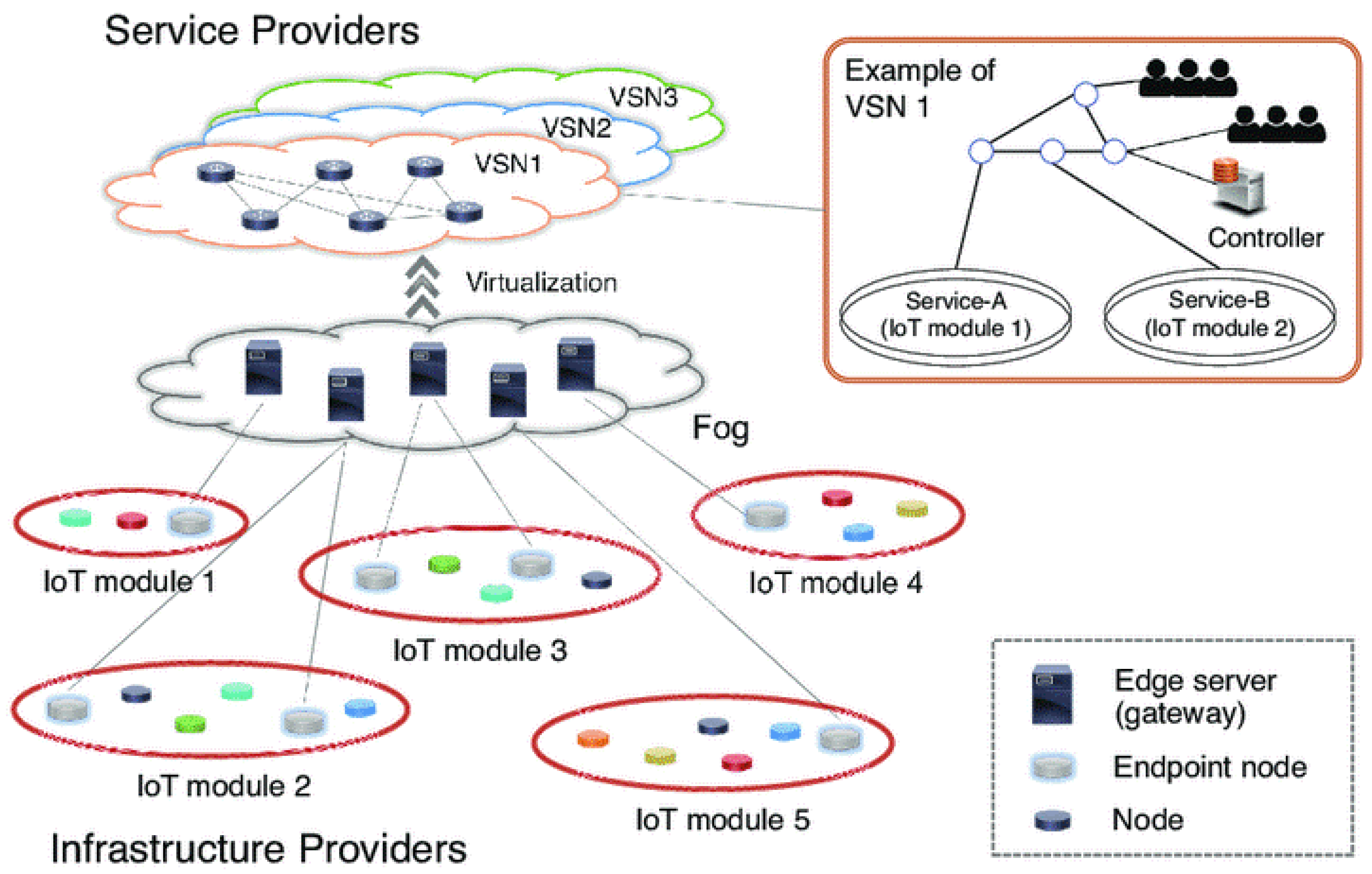
Sensing as a service (SaaS), which may be carried out in conjunction with network as a service (NaaS), is one of several fascinating application areas where the concept of WSN virtualization can be put to use. WSN virtualization enhances IoT security, resource usage, and administration, and decreases energy consumption [5]. Figure 1 shows how WSN visualization can be performed by making it easier for different kinds of networks to work together on the same physical infrastructure. The current four-tiered virtualization architecture for WSN networks is designed to cut down on unnecessary duplication of sensor networks across various IoT use cases [6,7,8].

The current virtualized wireless sensor networks architectures have not taken into account the possibility of a communication breakdown on a virtual network as a result of a breakdown in communications on real-world WSN networks. All nodes in a WSN are susceptible to failures such as node failures, communication failures, or internal component malfunctions of the sensors (such as a transceiver, CPU, battery, etc.) due to the wide variety of risk or hazard situations in which WSNs are deployed. Additionally to sensor attributes (low cost, compact size, high quality, etc.) [9], WSN technology has a number of challenges, but fault tolerance is by far the most significant of these. Due to the severity of these problems, it is even more important to include procedures and ways to remedy these flaws and reinforce their operation in order to boost fault tolerance [10].

In many scientific and technical contexts, it is important to simultaneously maximize many objectives while weighing the tradeoffs between them. Recent years have seen extensive studies devoted to the development of effective algorithms for resolving such multi-objective optimization (MOO) challenges. To solve MOO issues, these algorithms employ a population of candidate solutions, investigating a number of non-dominated solutions simultaneously. This is in contrast to the single-solution-at-a-time approach taken by conventional methods. In this process, the authors in [11] used a probabilistic approach to the formulation of a novel evolutionary multi-objective crowding algorithm (EMOCA). A middle ground between the issues of dominance and variety in the expanding population appears to be provided by their method.

In this context, this paper presents a novel architecture for heterogeneous virtual networks in the IoT that may be embedded into WSN settings to improve fault tolerance and decrease communication latency in service-oriented networking. Since fault tolerance and communication latency are often two conflicting objectives in WSN settings, the problem can be formulated as a reactive optimization of fault tolerance and communication delay, which in our case is carried out by adapting an evolutionary multi-objective crowding algorithm (EMOCA). EMOCA’s novel method lies in its use of a non-domination ranking scheme and a probabilistic technique to decide whether an individual’s offspring will be considered during the replacement-selection phase. EMOCA incorporates diversity preservation as an integral part of the algorithm. Compared with the well-known non-dominated sorting genetic algorithm NSGA-II, EMOCA discovers a diverse set of non-dominated solutions with near-uniform spacing [11]. Simulations are used to find out how well EMOCA performs at optimizing fault tolerance for virtualization in WSNs.

The remaining sections of the paper are as follows: the literature on virtual network embedding’s fault tolerance is discussed in Section 2. Section 3 lays forth the specifics of the multi-objective optimization problem’s mathematical formulation and EMOCA’s application toward resolving it. The simulation environment, metrics, and performance comparisons are discussed in Section 4, and a summary is provided in Section 5.

2. Related Works

This section will provide an overview of some of the studies that have been carried out on fault tolerance in virtual network embedding (VNE). We surveyed the literature and classified past research into three broad classes: that focusing on link failure, that focusing on node failure, and that focusing on multi-objective optimization for network survival. We will next move on to a discussion of virtualization as a contributing area in WSNs. Many approaches have been suggested to strengthen VNE’s dependability against the failure of the substrate resources, and many researchers have attempted to address the VNE problem using these mechanisms [12].

There are two main types of solutions to VNE survivability issues that have been identified in the literature: (a) proactive solutions that involve reserving resources in advance of a potential failure, and (b) reactive solutions that respond to a failure by immediately initiating a restoring mechanism [13]. In this case, each link’s backup-storage quota has been depleted to be used for protection and restoration. Survivability techniques based on connection restoration and protection are useful from a commercial standpoint, but they have certain limitations. In many instances, the reactive method might cause data loss. The survivability measurement also does not account for the fault-tolerance capabilities of connections or communication latency [13].

Reactive solutions utilize a path-selection algorithm to determine backup pathways for each underlying connection before any VNE request is received. An existing embedding technique is then used to create the virtual node and link it to the subsequent request. With increased data loads, failure can cause a significant loss of data, and the backup mechanism may not be able to restore the VNE [14]. In [15], the authors presented the link-based backup strategy as a preventative measure against link failure. A portion of each core link’s backup bandwidth is reserved in advance of any incoming VN request during the setup process. In this case, the backup bandwidth is scheduled ahead of time, before a problem occurs, which is preferable. Further, the VN embedding process requires fewer computational resources. With the shared pre-allocation method, backup bandwidth is held regardless of the VN requests, meaning it might not be used if even a small number of VN requests come at once.

To choose the most suitable virtual link for failure recovery, a hybrid technique was presented in [16]. In contrast to the reactive approach, which seeks to reallocate any capacity negatively impacted by a large request, the preventative approach embeds virtual links into numerous core channels to promote resistance to attacks and efficiency in resource use. This method depends on the WSN’s remaining hardware resources, which may not be enough to fix the virtual network on a very busy network. An approach for identifying the alternate link among the impacted virtual network (VN) resources is introduced in [17]. While a dynamic recovery method is useful in general, it is especially useful when physical failures cause additional downtime and resources are limited. This approach demands a full VN reset, which takes a long time and makes the service inaccessible.

The authors in [18] presented a two-step methodology for restoring the whole VN of the failed attachment node. First, a graph is built to request VN with a virtual link backup contract, and then the improved VN is requested on the core set by employing both the redundant and K-redundant schemes. While this strategy may help optimize the allocation of certain resources, it may not be able to do so for all of them. It is recommended to set aside a spare node and link for every vital node in the network. A second two-step strategy for restoring VN is presented in [19]. The VN is augmented using virtual nodes (V_Nodes) and virtual links (V_Links) in the first stage, and sensor networks are then given access to this improved VN in the second stage. In the worst event, each V_Node needs to have a backup set aside. The research in [20] offered an enhanced VN based on a failover method to minimize backup resources. Despite being resource-efficient, this method is unworkable because V_Nodes frequently migrate.

Contrary to these approaches, in [21], the authors presented a joint optimization approach to assign both primary and backup resources. Although heuristic-based mapping quickly tackles single-node failure, the complexity and inconvenience of considering backup resources and the possibility of node and connection failure are inherent in this embedding technology. A method for improving long-term viability with minimal operating expenses was discussed in [22], which takes advantage of the spatial distribution of VNE’s physical resources. A heuristic-based method was used for the smaller network, while an integer linear programming model was used for the larger one. It has been hypothesized that this is a multi-commodity network-flow issue. Since smaller networks often have faster physical connectivity, location data have less of an effect. If the structure of the virtual networks is altered, undesirable topology-based survival characteristics will emerge as a direct result. Even though there are more and more factors that take survival into account, the use of single-objective optimization approaches has stopped progress toward the best values for network parameters [23,24,25,26].

To improve fault tolerance in WSN virtualization, the popular MOO approach of non-dominated sorting based on a genetic algorithm (NSGA-II) is developed in [4]. Through a process of chromosomal sorting, NSGA-II is modified to address the optimization issue. The technique of sorting prioritizes chromosomes depending on competing criteria. Concerning solution dispersion and convergence to the genuine Pareto optimal, NSGA-II performs better than other Pareto-optimal approaches. However, there are drawbacks to the framework because of restrictions on the dissemination of consistency in some issues. Moreover, crowded comparisons can restrict the convergence. Virtualization proposals for WSNs tend to focus on improving resource (sensor) usage via the use of application-centric multitasking and the abstraction of sensors according to their use (i.e., virtual sensors).

The research in [27] investigated the challenge of finding the optimal lifetime and number of relay nodes for a network operating in three-dimensional environments. To achieve a better compromise between two goals, a new method is suggested. The technique combines a decomposition-based multi-objective evolutionary algorithm with a targeted local search to improve its component parts. In [28], the controller placement problem, which is a multi-objective optimization problem, is stated for selecting the optimal location for Software Defined Network (SDN) controllers to improve WSN performance. Considerations such as cost, time, and dependability are among the constraints that are applied here. In addition, a novel adaptive population-based cuckoo optimization (APB-CO) is used to position controllers optimally.

The work in [29] discussed WSN resource allocation for combined time-slot assignment, channel allocation, and power control. This study analyses resource dependency to design a two-stage resource-allocation optimization technique for a non-convex issue with diverse research aims and computing complexity. First, a graph-coloring technique for time-slot assignment is created for conflict-free sensor information interchange. Based on the first stage of this technique, combined power control and channel allocation are examined and articulated as a multi-objective optimization problem to solve the tradeoff between energy efficiency and network capacity maximization under link interference and load-balancing constraints. In their work, multi-objective hybrid-particle swarm optimization yields Pareto-optimal solutions.

In [30], the time function of the goal function perception matrix is presented, taking into account the features of low-power and real-time performance of sensor nodes in WSN. In order to limit the perceptual nodes’ inherent bias, a constraint on the number of targets they can detect is suggested; a weighted factor on the utility function is employed to ensure users are treated fairly; and finally, an optimization model of multi-objective resource allocation is established. To effectively allocate resources, a new technique is presented that builds on top of a modified version of simulated annealing (SA), bringing together the speedy optimization capabilities of SA with the robust search capabilities of logistic chaos.

The authors in [31] presented a multi-objective protocol (MOP) that maximizes network lifespan and residual energy using a mixed-integer linear-programming (MILP) optimization technique. Within the boundaries of the nodes that make up a given target, sets of MILP are solved locally. Therefore, within the same coverage nodes, energy is conserved. This research takes into account the goals of optimizing network residual energy and neighbor node connections. In order to determine which nodes to deactivate, each round’s local MILP solution is used to identify the nodes that have the lowest connection to their neighbors and are thus the most heavily used throughout the routing process.

For 5G systems that support the Internet of Things, the research in [32] developed a new method of clustering based on optimization via network slicing. By using network slicing and cluster construction, multi-objective improved seagull optimization-based clustering with network slicing (MOISGO-CNS) aims to improve 5G systems’ energy efficiency and load distribution. Both ISGO-based clustering and IGSO using bidirectional long short-term memory (BiLSTM) form the backbone of the MOISGO-CNS method. Two-hop connectivity ratio, residual energy, and link quality are the three metrics used to build a fitness function in the IGSO-based clustering method. In addition, the ISGO algorithm is developed as part of the network-slicing process in order to pick hyperparameters for optimum slicing classification performance. See [33,34] for an updated review of multi-objective optimization in wireless sensor networks. Recent studies that have looked at the crucial research of node and network-level virtualization in WSNs for the IoT [35,36] and applications show this to be the case [6,8,37,38,39].

In general, the problem with employing evolutionary algorithms for improving fault tolerance in WSN virtualization is that they cannot determine whether or not a solution is optimum; they can only determine whether or not it is “better” than other solutions that they already know about. It is also tricky to provide accurate weights to the objective functions, run the algorithm numerous times, and end up with various Pareto-optimal solutions; and Pareto-front concaves are notoriously difficult to analyze. A key challenge in the development of effective algorithms is the incorporation of diversity mechanisms into evolutionary algorithms for multi-objective optimization problems. This is the case for problems with an exponentially large number of possible non-dominated goal vectors. An acceptable approximation of the Pareto front is what we are aiming to obtain.

We look at how this can be carried out using the diversity mechanism of crowding dominance and highlight where this idea is demonstrably beneficial to handle internal failure perspectives in virtualization in WSNs. We use EMOCA as an MOO technique to maximize fault tolerance and minimize communication delay. The performance of EMOCA is compared with that of the well-known non-dominated sorting genetic algorithm NSGA-II. According to [11], EMOCA performs better than the other algorithm in eight of the nine test problems when it comes to convergence and diversity. It always finds a wide range of solutions that are not dominant.

3. The Proposed Framework

Here we cover the topic of virtualization’s fault tolerance in WSNs. We evaluate a network structure with four layers. There is the “physical” layer, which is made up of the real sensor nodes, and then there is the “virtualization” layer, which creates additional “virtual” sensors that can perform additional jobs and services beyond what the “physical” layer can. In the third layer, known as the “access layer”, different WSNs are developed based on the fault-tolerant incorporation of mission-oriented sensors. There is an access agent for every embedded network. The applications layer is where the IoT’s smart applications, such as humidity, fire monitoring, temperature, etc., are represented to the end users who really benefit from them. In order to implement the suggestion, the access layer is modified.

Every node in a traditional sensor network cooperates to deploy sensors at the same level [24]. When many sensor networks operate together and share the same physical location, they form the Virtual Sensor Network (VSN). The same domain hosts a variety of physically distinct sensor networks. As part of a larger wireless sensor network, it is established by the sensor nodes that are most relevant to a certain activity or use case at that moment [20]. But in a virtual sensor network, the nodes work together to complete a specified task at a precise moment. To create a virtual sensor network, logical connections must be made between cooperating sensor nodes. Depending on the phenomenon being monitored or the function being served, nodes may be organized into distinct virtual sensor networks. The capability for network construction, utilization, adaptation, and maintenance of a subset of sensors working on a given job should all be provided by the virtual sensor network protocol. The proposed framework’s flowchart is shown in Figure 2, and the mathematical terminology used to describe its key processes is included in

Table 1. Mathematical Nomenclature.

Notation	Description
$s^v$	Virtual source sensor of a link failure
$d^v$	Virtual destination sensor of a link failure
$s^p$	Source physical sensor
$d^p$	Destination physical sensor
$N^p$	Total number of paths between $s^p$ and $d^p$
$N_n$	Number of sensors in the network
$N_A$	Network area
$N_{in}$	Number of intermediate nodes between $s^v$ and $d^v$
$E\left(r\right)$	Expected closest-neighbor distance
$r$	Distance of nearest-neighbor sensor
$\mathsf{\Delta }r$	A small incremental distance in $r$
$\lambda$	Density of sensors in the network
$P_{r|\left(r+\mathsf{\Delta }r\right)}^c$	Probability of closest sensor between r and r + ∆r
$P_{r|\left(r+\mathsf{\Delta }r\right)}^s$	Probability of some sensor between r and r + ∆r
$P_{<r}^0$	Probability of no sensor at less than $r$ distance
$S_i$ or $S_{ij}$	The ith sensor or the jth virtualization of ith sensor
$f_{r^{\left(r\right)}}$	Probability density function (pdf) of closest-neighbor distance
$R$	Transmission range of sensors
$D$	Distance between $s^p$ and $d^p$
${\left(N_{in}-2\right)}_{ck}$	Number of paths with k intermediates
$F{T}_i^p$	Fault tolerance of ith path
$F{T}_i^l$	Fault tolerance of ith link
$C{D}_i^p$	Communication delay of ith path
$C{D}_i^l$	Communication delay of ith link
$C{H}_i$	The ith chromosome
$N_{re}$	Number of retransmissions for a success
$e_{i,j}$	Packet error rate of a link between nodes $i$ and $j$
$d_{i,j}^l$	Degree estimation of a link between nodes $i$ and $j$
$d_i^e$	Degree of ith node
$a$	Decision variable
$d_{i,j}$	Distance between nodes $i$ and $j$
$S_p$	Propagation speed
$S_t$	Transmission speed
$S_{pkt}$	Size of packet
$S^{pop}$	Size of chromosome population
$N^{gen}$	Number of generations during solution optimization
$l_{S,D}$	Link between $s^p$ and $d^p$
$F_i^{path}$	Fault tolerance of ith path
$D_i^s$	Dominance set of ith solution
$S_i$	The ith solution of the population
$np$	The number of solutions that dominate $p$
$F_j$	The jth front
$S^{child-pop}$	Size of child population
$R_i$	Rank of ith solution

.

Say we have a sensor network with nodes dispersed over the network region $N_A$. Assume mesh topology, meaning all nodes are connected. This network supports virtual networks. Assume a link-route breakdown causes $s^v$ and $d^v$’s link connection to fail. The wireless sensor network connects source physical sensor $s^p$ and destination physical sensor $d^p$ nodes. Investigate all possible paths between $s^p$ and $d^p$ to discover a fault-tolerant alternative. To find these routes, you must know the expected number of intermediary nodes. By calculating the average distance to the nearest-neighboring node, we may count the paths. Obtaining the sensor’s probability density function (pdf) is all that is required to compute the nearest-neighbor sensor’s distance; pdf is the probability of a neighbor sensor within $r$ and $\left(r+\mathsf{\Delta }r\right)$, where $r$ is the transmission radius and $\mathsf{\Delta }r$ is the incremental distance. The physical wireless sensor network is considered to have a uniform sensor distribution $\lambda$ such that [4].

$$\underset{N_A}{{\displaystyle \int }}\lambda d{N}_A=1\Rightarrow \lambda =\frac{1}{N_A}$$

(1)

For any two sensors separated by a distance between $r$ and $\left(r+\mathsf{\Delta }r\right)$, the probability $P_{r|\left(r+\mathsf{\Delta }r\right)}^c$ of the closest-neighbor sensor is equal to the product of the probabilities that one of the sensors is present at the distance $P_{r|\left(r+\mathsf{\Delta }r\right)}^s$ and that none of the other sensors are closer $P_{<r}^0$. Assume that the $N_n$ sensor nodes in the network can only send data at a distance of 0.5 rad to the destination $d^p$. In this case, $P_{r\mid \left(r+\mathsf{\Delta }r\right)}^c$ can be computed as:

$$\begin{array}{c}{P}_{r\mid \left(r+\mathsf{\Delta }r\right)}^c=P_{<r}^0\cdot P_{r\mid \left(r+\mathsf{\Delta }r\right)}^s\\ \end{array}$$

(2)

$$P_{r\mid \left(r+\mathsf{\Delta }r\right)}^c=\left[1-P_{<r}^s\right]\cdot \left[P_{r\mid \left(r+\mathsf{\Delta }r\right)}^s\right]$$

(3)

$$P_{r\mid \left(r+\mathsf{\Delta }r\right)}^c=\left[1-{{\displaystyle \sum }}_{j=1}^{N_n} \left(\begin{array}{c}{N}_n\\ j\end{array}\right){\left(\frac{\lambda \pi r^2}{2}\right)}^j{\left(1-\frac{\lambda \pi r^2}{2}\right)}^{N_n-j}\right].\left[{{\displaystyle \sum }}_{j=1}^{N_n} \left(\begin{array}{c}{N}_n\\ j\end{array}\right){{\displaystyle \int }}_r^{r+\mathsf{\Delta }r}{\left(\frac{2\lambda \pi r\cdot dr}{2}\right)}^{j}dr\cdot {{\displaystyle \int }}_r^{r+\mathsf{\Delta }r}{\left(1-\frac{2\lambda \pi r\cdot dr}{2}\right)}^{N_n-j}dr\right]$$

(4)

$$P_{r\mid \left(r+\mathsf{\Delta }r\right)}^c={\left(1-\lambda \pi r^2\right)}^{N_n}\left[1-{\left(1-\lambda \pi \left(rdr+d{r}^2\right)\right)}^{N_n}\right]$$

(5)

$$P_{r\mid \left(r+\mathsf{\Delta }r\right)}^c={\left(1-\lambda \pi r^2\right)}^{N_n}[1-\{1-\left(\begin{array}{c}{N}_n\\ 1\end{array}\right)\cdot \left(\lambda \pi \left(rdr+d{r}^2\right)\right)+ \left(\begin{array}{c}{N}_n\\ 2\end{array}\right)\cdot {\left(\lambda \pi \left(rdr+d{r}^2\right)\right)}^2\dots \}]$$

(6)

$$P_{r\mid \left(r+\mathsf{\Delta }r\right)}^c={\left(1-\lambda \pi r^2\right)}^{N_n}[N_n\lambda \pi rdr+N_n\lambda \pi d{r}^2-\left(\begin{array}{c}{N}_n\\ 2\end{array}\right)\cdot (\lambda \pi (rdr+{ d{r}^2))}^2\dots .]$$

(7)

In order to calculate the probability density function of the nearest-neighbor distance $f_r\left(r\right)$, we can use the limit in Equation (7) as:

$$f_r\left(r\right)=\underset{dr\to 0}{lim}\frac{P_{r\mid \left(r+\mathsf{\Delta }r\right)}^c}{dr}=N_n\lambda \pi r{\left(1-\lambda \pi r^2\right)}^{N_n}$$

(8)

Considering R as transmission range of sensors, the expected closest-neighbor distance (r) can be expressed as

$$E\left(r\right)={{\displaystyle \int }}_0^{R}r{f}_r\left(r\right)dr={{\displaystyle \int }}_0^R{N}_n\lambda \pi r^2{\left(1-\lambda \pi r^2\right)}^{N_n} dr$$

(9)

$$E\left(r\right)={\left[\frac{-r\left(1-\lambda \pi r^2\right)}{\lambda \pi \left(N_n+1\right)}\right]}_0^R+{{\displaystyle \int }}_0^R\frac{{\left(1-\lambda \pi r^2\right)}^{N_n+1}}{\lambda \pi \left(N_n+1\right)}dr$$

(10)

$$E\left(r\right)={\left[\frac{1}{\lambda \pi \left(N_n+1\right)}{{\displaystyle \sum }}_i^{N_{n+1}} \left({ }_{ i }^{N_n+1}\right)\frac{{\left(-\lambda \pi r^2\right)}^{i}r}{i+1}\right]}_0^R$$

(11)

$$E\left(r\right)=\frac{\sqrt{N_A}}{\lambda {\pi }^{\frac{3}{2\left(N_n+1\right)}}}{{\displaystyle \sum }}_i^{N_{n+1}} \frac{{(-1)}^i}{i+1}$$

(12)

It can be shown that there are exactly ${\left(N_{in}-2\right)}_{ck}$ pathways from $s^p$ to $d^p$ with exactly k intermediary nodes, where

$$k=\left\{1,2,3,\dots (⎣\frac{D}{E\left(r\right)}⎦-1 )\right\}$$

(13)

$$N_{in}=\left(⎣\frac{D}{E\left(r\right)}⎦-1 \right)$$

(14)

$D$ represents distance between $s^p$ and $d^p$. The equation for the total number of routes, $N^p$, from $s^p$ to $d^p$ is as follows:

$$N^p={\left(N_{in}-2\right)}_{C_1}+{\left(N_{in}-2\right)}_{C_2}+\cdots +{\left(N_{in}-2\right)}_{C_{\left(N_{in}-2\right)}}$$

(15)

$$N^p=\left\{{\left(N_{in}-2\right)}_{C_0}+{\left(N_{in}-2\right)}_{C_1}+\cdots +{\left(N_{in}-2\right)}_{C_{\left(N_{in}-2\right)}}\right\}-1$$

(16)

$$N^p=2^{N_{in}}-1$$

(17)

If we want to maximize fault tolerance (FT), we can write it as:

$$Maximize FT=\underset{i=1,2,\dots ,N^p}{max}\left(F{T}_i^p\right)$$

(18)

$$F{T}_i^p=\frac{1}{(⎣\frac{D}{E\left(r\right)}⎦-1)} {{\displaystyle \sum }}_{i=s^p ,j=1}^{i=(⎣\frac{D}{E\left(r\right)}⎦-1), j=d^p}F{T}_{i,j}^l$$

(19)

$F{T}_i^p$ is the fault tolerance of the ith path from source $s^p$ to destination $d^p$, and $F{T}_{i,j}^l$ is the fault tolerance of a link between an adjacent pair of nodes. The ordered set of nodes of ith path is represented by $S_i^{op}$

$$S_i^{op}=\{s^p, 1,2,\dots ,(⎣\frac{D}{E\left(r\right)}⎦-2), (⎣\frac{D}{E\left(r\right)}⎦-1), d^p\}$$

(20)

Similar to how the maximize FT function is written, the communication-delay (CD) minimization function is given by:

$$Minimize CD=\underset{i=1,2,\dots ,N^p}{min}\left(C{D}_i^p\right)$$

(21)

$$C{D}_i^p=\frac{1}{(⎣\frac{D}{E\left(r\right)}⎦-1)} {{\displaystyle \sum }}_{i=s^p ,j=1}^{i=(⎣\frac{D}{E\left(r\right)}⎦-1 ), j=d^p}\left(\frac{C{D}_{i,j}^l}{C{D}_{max}^l}\right)$$

(22)

$C{D}_i^p$ represents delay of ith path from $s^p$ to $d^p$, $C{D}_{i,j}^l$ is the delay of a link between an adjacent pair of nodes, and $i,j \in S_i^{op}$. The maximum link delay among all the links is represented by $C{D}_{max}^l$. The optimization issue outlined above has the following restrictions:

$$0<F{T}_i^p\le 1, 0<F{T}_i^l\le 1, 0<C{D}_i^p\le 1, 0<\frac{C{D}_{i,j}^l}{C{D}_{max}^l}\le 1$$

(23)

The problem can be formulated as a reactive optimization of fault tolerance and communication delay, which is accomplished in our case by adapting an evolutionary multi-objective crowding algorithm (EMOCA). The number of objectives being optimized for is the primary dividing line between single- and multi-objective streamlining. When there are several competing goals, there is no best way to solve the situation at hand. There are a few possible good solutions. Pareto-optimal solutions are those that maximize utility with the fewest costs. As far as all goals go, the Pareto front does not provide a single solution that is optimal. Accordingly, all Pareto-front solutions are valuable without any problem-specific knowledge regarding the relative importance of different goals. Finding numerous such solutions that represent tradeoffs between goals is the primary aim of multi-objective optimization [40,41].

The primary objectives of multi-objective evolutionary algorithms (MOEAs) include: (1) settling on a Pareto-optimal solution set; and (2) acquiring a wide variety of options that are evenly spaced. When solutions are distributed unevenly, the Pareto front becomes crowded in certain areas. The EMOCA solution prioritizes variety throughout the algorithm to solve this problem [11]. Evolutionary operators such as crossover and mutation, in addition to chromosomal sorting through the non-dominance concept and diversity, are used to alter the solutions in EMOCA. After multiple cycles, the EMOCA eventually arrives at a collection of tradeoffs known as the Pareto front. Unlike an aggregate optimization strategy that only offers one solution, this set of alternatives gives the system designer many to choose from. The main structure of EMOCA is illustrated in Algorithm 1. Now we will discuss each of EMOCA’s distinct steps [11].

Algorithm 1: EMOCA main structure

Initialize.  For the number of iterations determined by computational bounds, do: 2.1. Generate Mating Population. 2.2. Generate offspring by crossover followed by mutation. 2.3. Create a new pool consisting of parents and some offspring. 2.4. Trim new pool to generate the population for the next iteration. 2.5. Update archive to contain all non-dominated solutions

Mating Population Generation: As a means of increasing the number of viable mates, EMOCA uses a system of binary tournament selection. An individual’s fitness level is equal to their non-dominance rank plus their diversity rank. Individuals’ non-dominance ranks are determined using the non-dominated sorting algorithm presented in [42,43,44]. Each individual within the population is compared to the others to determine dominance. This gives initial non-dominated front solutions. The first front’s solutions are temporarily discarded, and then the preceding method is repeated until no non-dominated fronts remain. Solutions from the same non-dominated front are ranked equally.

For diversity rank, NSGA-II crowding’s distance metric determines each solution’s crowding density. To determine the density of solutions around a specific solution in a front, we calculate the average distance of two solutions along each goal (two solutions on either side of the solution $x_i$). Front boundary solutions have an infinite crowding distance. For all other solutions within a front, the following Algorithm 2 is used to assign the crowding distance [36]. Greater crowding distance in a solution suggests more variety (diversity). Based on their crowding distance, the solutions in the population are rated and ordered.

Algorithm 2: Crowding distance measure

For each solution $x_i$ of front F, initialize crowding distance $d\left(x_i\right)$ to be 0;  For each objective function $f_m$ do: 2.1 Sort the solutions in F along objective $f_m$; $\begin{array}{cc}d\left(x_i\right)=d\left(x_i\right)+& f_m\left(the individual that precedes xi in the sorted sequence\right)\\ & -f_m\left(the individual that follows xi in the sorted sequence\right)\end{array}$

New Pool Generation: After comparing each child to one of its randomly selected parents, taking dominance and crowding density into account, a new pool consisting of all the parents and some of the offspring is formed. Possible outcomes include the following three scenarios:

-

Case 1: The child gets introduced to the new pool if it is dominant over the parent.

-

Case 2: The probability of acceptance of the children is calculated using the crowding distance measure if the parent is dominant over the offspring. The probability P that a child will be included in the new pool if it has a larger crowding distance than its parent is:

$$P=1-exp\left(\left(\delta (parent\right)-\delta \left(offspring\right)\right)$$

(24)

$\delta$ denotes the crowding distance of a solution. A more diverse child with a larger crowding distance than its parent has a greater chance of survival. More diverse solutions are rewarded by being given a chance to thrive in subsequent generations.

-

Case 3: In cases where the parent and offspring are not dominant over one another, the offspring will be included in the new pool if its crowding distance is greater than that of the parent.

Trimming New Pool: Both non-domination rank and diversity rank are used to sort the new pool. Thus, the diversity rank is used to compare alternatives that have the same non-domination rating. The new population will be made up of the initial items of the sorted list of fronts $F_1$, $F_2$,…, $F_{\mathrm{n}}$ where elements of $F_i$ + 1 are dominated only by elements in $F_1$, $F_2$, …, $F_i$. All generations of non-dominated solutions are saved in EMOCA’s archive.

For the most part, EMOCA relies on an individual’s diversity score to determine whether or not their offspring will be allowed to join the new population. While EMOCA does not tolerate offspring who are dominant like their parents, it does allow some low-quality offspring to remain in the population, provided they have sufficient variety. The result is a more well-rounded and interesting population. Although NSGA-II allows all viable offspring to go on into the next generation, EMOCA only allows a small percentage to do so. Therefore, whereas NSGA-II executes non-dominated sorting on a population of size 2N, where N is the population size, EMOCA executes non-dominated sorting on a population size between N and 2N. With this, EMOCA’s computational complexity decreases [11].

3.1. Chromosome Representation

In EMOCA’s solution space for an optimization problem, a chromosome $C{H}_i$ is an ordered collection of intermediate nodes $S_i^{op}$ that begins with source $s^p$ and ends with $d^p$. Genes in the chromosomal model are represented by each node in the set.

$$C{H}_i={\left\{s^p,1,2,\dots ,\left(\left[\frac{D}{E\left(r\right)}\right]-2\right),\left(\left|D/E\left(r\right)\right|-1\right),d^p\right\}}^{FT,CD}$$

(25)

$$F{T}_{i,j}^l=\left(1-{{\displaystyle \sum }}_{t=0}^{N_{re}} {\left(e_{i,j}\right)}^t\left(1-e_{i,j}\right)\right)+d_{i,j}^l$$

(26)

Given a connection with packet error rate $e_{i,j}$ and degree estimate of the link $d_{i,j}^l$, we may calculate the number of retransmissions, $N_{re}$, that will be necessary for a successful transmission. In this case, a path’s cumulative fault tolerance is calculated by adding the fault tolerances of its individual connections. With the help of packet-error-rate-based link-quality estimation and neighbor-density-based degree estimation, we are able to calculate a link’s fault tolerance $F{T}_{i,j}^l$. The degree estimation can be derived from Equation (27) where $d_i^e \mathrm{and} d_j^e$ are the degrees of nodes $i$ and j, respectively, and $\alpha$ is a decision variable varying between 0 and 1.

$$\begin{array}{c}{d}_{i,j}^l=\{\begin{array}{cc}1, & d_i^e=d_j^e=N_n-1\\ 1-{\alpha }^{d_i^e}, & d_i^e=d_j^e<N_n-1\\ 1-{\alpha }^{\frac{{\left(d_i^e-d_j^e\right)}^2}{d_i^e+d_j^e}},& \left|d_i^e-d_j^e\right|>0\end{array}\\ \end{array}$$

(27)

When calculating the communication delay $C{D}_{i,j}^l$, we factor in interference for the connection, which is based on the link quality, as well as propagation and transmission delay where $d_{i,j}$ is the distance between the pair of nodes $i$ and $j$, $S_p$ represents propagation speed, $S_{pkt}$ is the packet size, and $s_t$ represents transmission speed.

$$C{D}_{i,j}^l=\left(1-{{\displaystyle \sum }}_{t=0}^{N_{re}} {\left(e_{i,j}\right)}^t\left(1-e_{i,j}\right)\right)+\frac{d_{i,j}}{S_p}+\frac{S_{pkt}}{s_t}$$

(28)

3.2. Crossover and Mutation

The crossover procedure involves randomly swapping a collection of nodes between two chromosomes from the population (all paths between $s^p$ and $d^p$). The exchange is limited to nodes that are reachable both downstream and upward. Larger group sizes are desirable in the earlier stages (lower generations) of a solution. Generation number and chromosomal pair size determine crossover group size. Due to the recurrence of intermediate nodes, chromosomes after crossover operations (also called offspring in optimization theory) are repaired. Intermediate nodes in the parent chromosome but not in the offspring are considered during repair. If two randomly chosen nodes on the chromosome can be reached (present as neighbors) from their respective descendant nodes, then the mutation process will swap their positions.

3.3. Non-Dominance and Crowding-Distance-Based Sorting for Chromosomes

Using non-dominance, chromosomes are sorted. Multiple competing goals are used to arrange chromosomes. Consider population chromosomes $C{H}_i$ and $C{H}_j$. According to Pareto optimum, a chromosome $C{H}_i$ dominates $C{H}_j$ if at least one of its fitness values is higher than CH_j’s and the other fitness values are equal. Multi-objective optimization in communication networks favors Pareto-optimal prioritizing [40,41]. For two goals, it is:

$$C{H}_i>C{H}_j=\{\begin{array}{l}C{H}_i\left(FT\right)>C{H}_j\left(FT\right),\wedge C{H}_i\left(CD\right)\nless C{H}_j\left(CD\right)\\ C{H}_i\left(CD\right)>C{H}_j\left(CD\right),\wedge C{H}_i\left(FT\right)\nless C{H}_j\left(FT\right)\end{array}$$

(29)

The population’s chromosomes are sorted by fitness using the non-dominance notion. Non-dominant chromosomes rank first in the population. Only one chromosome in a population ranks second. Population-wise, chromosomes dominated by two others rank third. Each chromosome’s crowding distance is computed after ranking. The next generation is chosen via a tournament method.

Algorithm 3 lays out the whole process that was followed to obtain an optimal solution, for which a population (paths between pairs of sources and destinations) of size $S^{pop}$ is formed by randomly scattering the decision variable throughout some allowed range (low, high). Non-dominance-based sorting $ol{d}^{pop}$ is used to order the population. To determine the objective-1 normalized fault tolerance and the objective-2 normalized delay for each $S_i\in ol{d}^{pop}$, the best half of the population is selected, and for each $S_i$ the crowing distance $C^{dist}$ is computed from all points excluding boundary points. Using the tournament-selection approach, the best half of the population is chosen based on the rank of $i^{th}$ solution $R_i$ and crowding distance $C^{dist}$. By introducing mutations and performing crossovers, a superior solution may be generated from a preselected parent population. The optimal half of the population is once again chosen from the whole population. These procedures are iterated until the stop criterion is met (the maximum number of generations is reached) in order to produce optimal chromosomes. The time complexity of EMOCA is $O(2\times S^{pop}\times N^{gen}$), where $S^{pop}$ is size of the old population and $N^{gen}$ represents the number of generations. The number of generations, and hence the amount of time it takes to run, is indirectly determined by the size of the network. As a result, the time needed for each generation might change based on the system’s hardware.

In summary, convergence is emphasized by the concept of non-domination rank. During the period of tournament selection and population reduction, variety is preserved by the use of diversity rank. It is also possible to apply the crowding distance to the parameter space [11]. In contrast, we measure crowding in the target space to determine the optimal solution. When compared to NSGA-II and other multi-objective evolutionary algorithms (MOEAs) such as multi-objective ant-colony optimization (MOACO) and multi-objective particle-swarm optimization (MOPSO), EMOCA’s most distinguishing features include:

-

When selecting whether or not to include a new generation into the population, EMOCA takes into account each individual’s diversity score. In contrast to MOEAs, which eliminate offspring who take after a single parent, EMOCA lets some low-quality offspring to persist in the population so long as they contribute to genetic variety. In a nutshell, this contributes to a more diverse population.

-

While NSGA-II allows all viable offspring to go on into the next generation, EMOCA allows just a small percentage to do so. Thus, whereas NSGA-II can only carry out non-dominated sorting on a population of size 2N, EMOCA can perform non-dominated sorting on populations with sizes ranging from N to 2N. The computational burden placed on EMOCA is therefore decreased.

-

In EMOCA, both non-domination and diversity are equally weighted by a single measure (the total rank) used for mate selection. This tremendously aids efforts to diversify and improve the quality of the available mating pool. But MOEAs and NSGA-II employ non-domination rank as the major criterion for selecting the mating pool. As a result, the resulting mate pool could not be as diverse as it otherwise would be.

Algorithm 3: EMOCA for solving the optimization problem

Input:$S^{pop}$, $N^{gen}$, $l_{S,D}$, $F_i^{path}$ Starting with generate initial population size $S^{pop}$. Then saving one copy of population as “$ol{d}^{pop}$”. For each $S_i$ ∈ $ol{d}^{pop}$     Calculate objective-1 normalized fault-tolerance using Equation (19)    Calculate objective-2 normalized delay using Equation (22) End for  $\mathrm{g}$ = 1; While $\left(\mathrm{g} \le N^{gen}\right)$    Non-dominated sorting ($ol{d}^{pop}$)   For each $S_i$ ∈ $ol{d}^{pop}$    Calculate $D_i^s$  End for     j = 1,  For each $S_i$ ∈ $ol{d}^{pop}$     If ($D_i^s=\varphi$)     $F_j=F_j\cup S_i$, $R_i=1$    End if  End for     j = 2,  For each $S_i$ ∈ $ol{d}^{pop}$  If ($D_i^s\ne \varphi \&\& R_i==j-1)$  $F_j=F_j\cup S_i$, $R_i=1, j=j+1$  End if End for Crowding _distance ($ol{d}^{pop}$)  Assume $C^{dist}$ from boundary point (group of solution) to ∞ for any solution.  For each $S_i$ ∈ $ol{d}^{pop}$     Calculate $C^{dist}$ from all point excluding boundary points  End for  Select the best half population as $paren{t}^{pop}$ considering $R_i$ & $C^{dist}$ using tournament selection approach.    $chil{d}^{pop}$ = $\varphi$    $S^{child-pop}$ = 0  While ($S^{child-pop}$ ≤$S^{pop}$)    Randomly select two chromosomes from the parent population.    Perform crossover to produce two child chromosomes.    Update $chil{d}^{pop}$ and $S^{child-pop}$ = $S^{child-pop}$ + 2    Randomly choose a chromosome from parent population.    Mutate chromosome to produce a child chromosome    Update $chil{d}^{pop}$ and $S^{child-pop}$ = $S^{child-pop}$ + 1  End while    Generate new population of size (2 × $S^{pop}$) by $ol{d}^{pop}$ ∪ $chil{d}^{pop}$    Calculate normalize fault-tolerance using Equation (19).    Calculate normalized delay using Equation (22).    Non-dominated sorting ($Nol{d}^{pop} \cup chil{d}^{pop}$)    Crowing_ distance ($ol{d}^{pop} \cup chil{d}^{pop}$)    Select again the best half population as $ol{d}^{pop}$ using rank and $C^{dist}$ End while Output: optimized chromosomes

The next section details the simulations run to assess the framework’s efficacy, paying special attention to the parameters of the test beds, the metrics used, and the analysis of the resulting data. Two goals were set to accomplish simulations based on case studies. To begin, the number of generations has an influence on fault-tolerant optimization’s efficacy, which is then used to determine how well it performs. Second, network density is a key indicator of fault-tolerant optimization’s effectiveness.

4. Experimental Results

In order to evaluate the proposed framework in virtual networks, the NS2 network simulator employs C++ to develop the simulation’s primary classes. The major classes of the simulation include ‘NetworkNode’, ‘VirtualNode’, ‘RandomProvider’, ‘PathSearch’, and ‘MainApp’. All the characteristics of a node in a network, such as position, list of neighbors, link delay with neighbors, and fault tolerance of associated links, are implemented in ‘NetworkNode’. At ‘VirtualNode’, tasks are processed using an interface-based architecture. Different sets of network nodes are generated at random by the ‘RandomProvider’ for each simulation run. PathSearch is a tool for optimizing virtual network generation with respect to delay and fault tolerance. The simulation is run on a machine with a 64-bit UBUNTU operating system (Linux), 16 GB of RAM, and an Intel Core i7-11700K processor running at 3.6 GHz. Three sets of randomly formed networks of 100, 500, 1000, 1500, and 2000 nodes are constructed using the Poisson distribution method. For each of four distinct networks, the EMOCA algorithm is run for 500, 1000, 1500, and 2000 generations in an effort to maximize fault tolerance and minimize communication latency. The most recent generation’s chromosomes in the results table stand in for the most recent set of optimized values.

Parameter and setting values utilized in the simulations are listed in

Table 2. Basic parameter setting for simulation.

Parameter	Value
Simulation area	$1500{ \mathrm{m}}^2$
Simulation time	$600 s$
Number of nodes	$100-1000$
Bandwidth	$40 \mathrm{Kbps}$
Transmission range	$15 \mathrm{m} \mathrm{to} 30 \mathrm{m}$
Receiving range	$15 \mathrm{m}$
Initial node energy	30 $\mathrm{J}$
Packet type	$\mathrm{UDP}$
Channel type	$\mathrm{Wireless}$
Antenna model	$\mathrm{Omni}$
MAC protocol	$\mathrm{IEEE} 802.11$
Query period	$3 s$
Hello timeout	$1 s$

. Sensors are deployed in a range of 100 to 1000, according to a specific deployment pattern, with a maximum transmission radius of 30 m, uniformly and randomly distributed across the circle with area $N_A=1500{ \mathrm{m}}^2$. The initial energy level J of each sensor is the same. The power consumed while transmitting, receiving, and in the idle state are 175 mJ, 175 mJ, and 0.015 mJ, respectively. The power consumed for sensing is equal to 1.75 $\mathsf{\mu }\mathrm{J}$. For focusing on coverage measurement, a sensing range of 10 m and a transmission range of 30 m are considered during the simulation. Transmission delays due to propagation have been deemed insignificant for the simulation region chosen. Each experiment was repeated 30 times using the specified simulation settings and variables, and the arithmetic mean was used to optimize the data record with a 95% degree of confidence.

4.1. Comparative Results

In Figure 3, Figure 4, Figure 5 and Figure 6, we see how EMOCA, NSGA-II, and multi-objective versions of both optimization algorithms, which include particle-swarm optimization (PSO) and ant-colony optimization (ACO), perform while optimizing a network with 100 nodes across 500–2000 generations. Herein, the comparative algorithms were employed as black-box versions with their default parameters (open-source code from GitHub). It is evident that EMOCA outperforms other comparative algorithms in terms of optimization performance, with regards to both fault tolerance and communication latency. The finding demonstrates that virtualized WSNs based on EMOCA can successfully deal with failure. More specifically, the optimal values for fault tolerance and communication latency are 0.67 and 0.02, respectively. This is because packet-error rate is a reliable predictor of fault tolerance. For the multi-objective version of ACO, the optimal value of fault tolerance is approximately 0.57 and the optimal value of communication delay is approximately 0.038. However, for the multi-objective version of PSO, the optimal values of fault tolerance and communication delay are 0.31 and 0.11, respectively.

The optimal value of fault tolerance for NSGA-II is around 0.44, whereas the optimal value of delay is approximately 0.05. This is because a fault-tolerant estimate is reliant on the degree of connection. In a wireless environment, the estimate is inappropriate. Having a large number of chromosomes also increases latency and decreases fault tolerance. In addition, because of the reduced size of the network (100 nodes), the effect of a larger number of generations on the final, optimized chromosome is far less dramatic. It is difficult to tell what makes one set of results distinct from the next. This is because there are fewer possible paths to create in more compact networks.

The network is scaled up to 500 nodes in order to amplify the optimization performance gap between generations. Figure 7, Figure 8, Figure 9 and Figure 10 display a comparison of optimization performance with increasing network size. The results show that when both goals are included, EMOCA achieves greater optimization performance than NSGA-II and multi-objective versions of both ACO and PSO. Specifically, the fault tolerance value of the latest optimized chromosome is about 0.92, while the communication latency value is around 0.015. This is because more paths are available in more extensive networks, allowing for the selection of connections of higher quality, with higher fault tolerance and reduced communication latency. There is a tradeoff between fault tolerance and communication latency, with the optimal value for each ranging around 0.82, 0.06 for ACO; 0.72, 0.08 for NSGA-II; and 0.59, 0.1 for PSO, respectively. The pace at which the system converges on an optimal solution has slowed, and the number of optimized chromosomes has decreased. Additionally, the bigger network (500 nodes) mitigates the negative effects of increasing the number of generations on the optimized chromosome.

The convergence rate toward the ideal solution is boosted by increasing the network size to 1000 nodes. Figure 11, Figure 12, Figure 13 and Figure 14 display a comparison of the optimization convergence rates. As expected, the results show that EMOCA has a higher optimization convergence rate compared to NSGA-II, ACO, and PSO for both goals. Comparatively, the optimum chromosomal value for communication latency is about 0.010, whereas the fault-tolerance value is around 0.98. This is because, as the size of the network grows, more and more paths become suitable for use, allowing for more discriminatory tolerance in the paths that are ultimately chosen. The optimal fault tolerance for ACO chromosomes is around 0.82, whereas the optimum communication delay is about 0.06. The optimal fault tolerance for NSGA-II chromosomes is around 0.78, whereas the optimum communication delay is about 0.07. The optimal fault tolerance for PSO chromosomes is around 0.59, whereas the optimum communication delay is about 0.1. In addition, when the size of the network is ramped up, the proportion of optimized chromosomes grows. In both cases, you will find that the chromosomes are packed closely together. We can also observe that the Pareto front obtained by EMOCA covers a wider region of the objective space compared to the Pareto fronts obtained by the other algorithms.

4.2. Summary of Results

We can also observe that the Pareto front obtained by EMOCA covers a wider region of the objective space compared to the Pareto fronts obtained by the other algorithms. EMOCA yields much smaller values for the crowding distance of a solution compared to competing techniques. EMOCA finds a wide variety of non-dominated solutions spaced out almost uniformly. These characteristics enable EMOCA algorithms to search for solutions in a much larger space with less complexity, and the results show that the EMOCA approach was capable of providing more accurate solutions at a lower computational complexity than the existing compared methods.

Algorithms built on the NSGA-II framework outperform their PSO-based counterparts. Here are several explanations that might be at play. Because of NSGA-II’s crossover and mutation processes, chromosomes may be shifted across huge distances in the solution space. Additionally, in NSGA-II, there is no correlation between individual chromosomes and the present local or global best results. Such capabilities allow NSGA-II based VNE algorithms to explore solutions in a considerably broader area than is possible with the PSO method alone. On the other hand, only the “best” particle shares its knowledge in PSO-based VNE algorithms. In contrast to PSO-based algorithms, those based on ACO vary in the calculation rank of the nodes, which affects the sequence in which virtual node consolidation and pheromone computing occur. As a result, EMOCA algorithms are a viable option for multi-objective optimization since they may provide more workable solutions.

5. Conclusions and Future Work

Both diversity and convergence are crucial for VNE optimization techniques. A system designer who is interested in analyzing several tradeoff alternatives in order to make an informed decision would not benefit from a Pareto set with few solutions concentrated in a certain location of the Pareto front. In this study, we demonstrate how we optimized two conflicting objectives—fault tolerance and communication latency in virtualized WSNs—by concentrating on heterogeneous network requirements for IoT applications through utilizing an EMOCA framework that uses a stochastic replacement-selection technique that includes both non-domination and diversity. In order to address the issues of fault tolerance and communication latency in virtualized WSNs, a mathematical formulation of a multi-objective optimization problem is presented. Using NSGA-II as a benchmark, we found that EMOCA’s optimization framework was superior to the current standard. Simulation results demonstrate that EMOCA outperforms superior optimization techniques produced with fewer generations. Moreover, the time to achieve the optimization outcomes is reduced compared to the best current methods. This proves the effectiveness of the suggested framework in terms of convergence and diversity, since a diverse range of non-dominated solutions is constantly discovered. The successful performance of EMOCA in optimization challenges across a broad range of sectors, such as routing and battery life in virtualized WSNs, will be considered in future research work. This is in addition to expanding the current work to include many other objective functions besides fault tolerance and communication delay.