Active Fault-Tolerant Control Applied to a Pressure Swing Adsorption Process for the Production of Bio-Hydrogen

Abstract

Pressure swing adsorption (PSA) technology is used in various applications. PSA is a cost-effective process with the ability to produce high-purity bio-hydrogen (99.99%) with high recovery rates. In this article, a PSA process for the production of bio-hydrogen is proposed; it uses two columns packed with type 5A zeolite, and it has a four-step configuration (adsorption, depressurization, purge, and repressurization) for bio-hydrogen production and regeneration of the beds. The aim of this work is to design and use an active fault-tolerant control (FTC) controller to raise and maintain a stable purity of 0.9999 in molar fraction (99.99%), even with the occurrence of actuator faults. To validate the robustness and performance of the proposed discrete FTC, it has been compared with a discrete PID (proportional–integral–derivative) controller in the presence of actuator faults and trajectory changes. Both controllers achieve to maintain stable purity by reducing the effect of faults; however, the discrete PID controller is not robust to multiple faults since the desired purity is lost and fails to meet international standards to be used as bio-fuel. On the other hand, the FTC scheme reduces the effects of individual and multiple faults by striving to maintain a purity of 0.9999 in molar fraction and complying with international standards to be used as bio-fuel.

1. Introduction

Hydrogen is the most abundant element in nature. It is a compound that generates a large amount of energy. By purifying this compound (bio-hydrogen) and obtaining it with a high degree of purity, it can be used in industrial processes for energy applications, such as fuel cells used to power cars, buses, trucks, railways, ships, and planes, or as backup power in stationary modules [1,2,3,4,5]. The need and availability of this compound as an alternative energy source is essential for the world; as a result, several industries have combined various hydrogen production processes, obtaining it with a low $C{O}_2$ emission, therefore helping to reduce atmospheric pollutants [6,7,8].

Bio-hydrogen is not only a source of energy, but can also be used to store it and can be distributed in various channels for a wide range of decarbonization applications, from reducing fuel emissions in vehicular transport to helping reduce the carbon footprint of traditionally carbon-intensive industries [9,10,11].

There are several ways to produce bio-hydrogen, one of them being the pressure swing adsorption (PSA) process, which uses two columns packed with adsorbents (natural or synthetic) to purify and separate the compounds from a mixture [12,13,14,15,16,17,18]. However, the PSA process is a complex technology represented by partial differential equations (PDEs) with a cyclical nature, in which various variables interact such as pressure, temperature, flow and composition. These variables can be affected at the input of the process by unknown disturbances, causing a low recovery and production of bio-hydrogen, and, consequently, a product that does not meet the international standards to be used as bio-fuel is obtained [19,20].

Therefore, it is important to consider automatic controllers in this type of highly non-linear process (rigorous PSA model) that can maintain system stability and help mitigate certain disturbances that appear at the input. There are some innovative works related to the control of the PSA process for the production of bio-hydrogen, one of them being the one reported by [21], in which they established an EMPC (economic model predictive control) strategy. The novel artificial intelligence algorithm manages to study computational cost optimization problems and propose control signals over a PSA process. They designed a scheme using a neural network to capture the dynamic behavior of the process. The EMPC managed to generate higher $CO$ purity by attenuating the disturbances presented at the entrance of the PSA process [22,23,24,25,26,27,28]. Later in the work presented by [29], a state feedback control over a PSA process for the production of bio-hydrogen was designed. The objective of the controller is to bring the hydrogen purity to 0.99 molar fraction and maintain the desired purity, even in the presence of disturbances [30]. Comparisons were made with a discrete PID (proportional–integral–derivative) controller based on an identified Hammerstein–Wiener model. The different disturbances that occurred in the virtual PSA plant were attenuated, achieving the maintenance of a purity above 99%, even when there are combinations of disturbances. The product they obtained complies with international bio-fuel standards.

There are very few works related to the control of the PSA process for the production of hydrogen, and the little information that exists presents controller schemes that only follow the trajectory without assuming disturbances that may exist in the feed. These disturbances have a great impact on the process since they can cause the purity of hydrogen to decay to a point where the entire system cannot return to the desired purity on its own, and that would mean that the product obtained cannot meet the international standards to be used as bio-fuel. However, there are works on PSA control for the production of medical oxygen and bio-ethanol, which have a great contribution to the literary follow-up on the development of this article. One of them is the one presented in [31]. They recently implemented the multivariable model predictive controller (MPC) on a single-bed medical oxygen concentrator (MOC). The method used to adsorb and desorb the molecules is rapid pressure swing adsorption (RPSA). A state space model was used to design an MPC. The linear model was identified using the MatLab ToolBox; they also generated an algorithm to optimize and reduce the error taken by the MPC controller. The variable was manipulated (duration of the steps) in real time to control the purity obtained (purity of hydrogen). On the other hand, Ref. [32] focuses on the design and application of two types of controllers to evaluate efficiency and performance. These controllers are the fault-tolerant control (FTC) and the fuzzy PID applied to the PSA process for bio-ethanol production. Both controllers achieved stabilization and follow the desired trajectory, as well as eliminating constant-type faults. However, the discrete PID controller failed to quickly stabilize the purity in the event of a variable fault and consequently only obtained purity values of 88.4% wt of ethanol. The FTC reached a purity of 99.5% wt of ethanol before the same tests proposed with the discrete PID control, which allows the product obtained with the FTC to be used as bio-fuel. Another of the works found is the one reported in [33], where the control problem of a PSA unit was studied using a robust stabilizing infinite-horizon model predictive (RIHMPC) strategy with a capacity for realistic mismatch scenarios. They evaluated the controllability of a PSA process and used a titanium terephthalate adsorbent combined with a MIL-125 porous amino to separate a synthesis gas. The controller (RIHMPC) they designed demonstrated great performance given the complexity of the highly nonlinear model and its cyclical nature.

The main contribution of this work is focused on designing and validating a discrete active FTC, which aims to reduce the effect of faults that occur on the PSA process for the production of bio-hydrogen. It is important to mention that this designed controller is robust to different types of faults that occur on the actuator (production valve), allowing the purity to meet the international standards for use as bio-fuel, achieving a purity of 0.999% in the molar fraction.

This work is sectioned as follows: Section 2 presents the main characteristics of the PSA process and the modeling used for the production of bio-hydrogen. Section 3 presents the simulations from the start-up to the cyclic steady state (CSS), showing the behavior of the compositions, pressure, and temperature. In Section 4, the reduced model (Hammerstein–Wiener) is established. Section 5 shows the design of the active fault-tolerant controller implemented in the Hammerstein–Wiener model and its structure. Finally, the results and discussions are presented in Section 6.

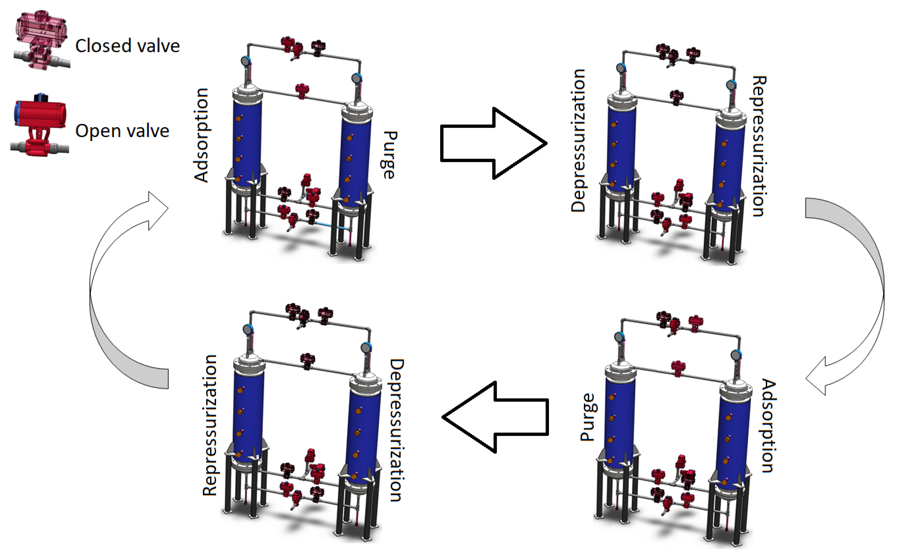
2. Characteristics and Configuration of the PSA Process for the Production of Bio-Hydrogen

The PSA process consists of two columns made of stainless steel that are placed in parallel. Both columns have pressure and temperature sensors. Columns are packed with zeolite type 5A. In order to make the process work cyclically, eleven valves were placed that let the steam flow through and generate the adsorption, depressurization, purge, and repressurization steps. The PSA process has a feed of 0.162 kmol kmol⁻¹, with a concentration in a molar fraction of 0.11 ($CO$), 0.61 ($H_2$), and 0.28 ($C{H}_4$). The production pressure used is 980 kPa with a temperature of 298.15 K. The purge pressure used is 100 kPa (see Figure 1).

The operation cycle of the PSA process for the production of hydrogen includes four steps: adsorption, depressurization, purge, and repressurization (see Figure 2). The first step is carried out synchronously between Bed 1 (B1) and Bed 2 (B2); while B1 is adsorbing and producing hydrogen, B2 is purging to release the active sites of the 5A zeolite. The second step is carried out in the same period of time; while B1 is depressurizing, B2 begins to repressurize to be ready for the hydrogen adsorption and production step. In the case of the third step, B1 begins to purge and B2 begins adsorption, and for the fourth step, after purging, B1 begins repressurization so that it can once again adsorb and purify hydrogen while B2 is carrying out the depressurization oscillating from high to low pressure.

The established configuration (valve opening) for the steps and the adequate execution time are established by the pressure profile that occurs within the packed columns because if a longer time is set, it can cause the bed to saturate and fail to adsorb and produce bio-hydrogen. In the same way, for the depressurization and purge step, it is necessary to establish short times for regeneration since this favors the release of the adsorbed $CO$ and $C{H}_4$ molecules, and once again, the bed can be ready to adsorb.

Non-Linear Model of the PSA Process for the Production of Bio-Hydrogen

The modeling and simulation of PSA processes for hydrogen production are necessary tools to study and describe the dynamic behavior of the purification and production of compounds or gases. This research is related to packed columns or beds, the configuration of the steps to establish the operation cycle, nominal start-up conditions, and observing the critical points in the PSA process. For this case study, a PSA process is established that contemplates the following assumptions:

• There are no reactions between the elements of the mixture ($H_2,C{H}_4$ and $CO$).
• The steam phase is convective and axial dispersion is constant.
• The Langmuir model is used in terms of partial pressure.
• The mass transfer coefficient is considered constant.

Based on these assumptions, the equations to be used considering the proposed characteristics are established. These are described in

Table 1. Equations used for modeling the PSA process and hydrogen production.

Equation	Description of Contributions
	Material balance accounts for
Mass balance for gas phase	Convection
	Dispersion
	Accumulation
	Energy balance accounts for
Gas phase energy balance	Thermal conduction (Solid)
	Heat of adsorption
	Heat transfer (Gas–solid)
	Momentum balance accounts for
Pressure drop	Karman–Kozeny
	Burke–Plummer
	Ergun equation
	Kinetic equilibrium
Kinetic models For solid	Linear Driving Force (LDF)
	Diffusion Pore
	Mass Transfer Coefficient (Constant)
	Thermodynamic equilibrium
Langmuir	Isotherm assumed for layer (Extended Langmuir 3)

.

The mathematical model of the PSA process for the production of hydrogen is developed by using the following equations:

• Mass balance equation:

$$-D_L\frac{{\partial }^2{c}_i}{\partial z^2}+\frac{\partial \left(U_z{c}_i\right)}{\partial z}+\frac{\partial c_i}{\partial t}+\frac{(1-{ϵ}_b)}{{ϵ}_b}-\rho \frac{\partial W_i}{\partial t}=0.$$

(1)

• Energy balance equation:

$$K_L\frac{{\partial }^{2}T}{\partial z^2}+\left[{ϵ}_{b}c{C}_{pg}+(1-{ϵ}_b){\rho }_p{C}_{ps}\right]\frac{\partial T}{\partial t}-{ϵ}_{b}c{C}_{pg}{U}_z\frac{\partial T}{\partial z}=(1-{ϵ}_b){\rho }_p\sum _{j=1}^N\mathsf{\Delta }{H}_j\frac{\partial n_j}{\partial t}+\frac{2h_{in}}{R_{in}}(T_w-T).$$

(2)

• Ergun equation for momentum balance:

$$-\frac{\partial P}{\partial z}=\left(\frac{150\mu V_z{(1-{ϵ}_b)}^2}{4R_p^2{ϵ}_b^3}+\frac{1.75{\rho }_g(1-{ϵ}_b)}{\left(2R_p\right){ϵ}_b^3}{v}_g^2\right).$$

(3)

• Equation of kinetics:

$$\frac{\partial W_i}{\partial t}=MT{C}_{si}(W_i^{*}-W_i),MT{C}_{si}=\frac{\mathsf{\Omega }{D}_{ei}}{r_p^2}.$$

(4)

• Adsorption isotherms:

$$W_i^{*}=\frac{(I{P}_1-I{P}_2{T}_s)I{P}_3{e}^{i{p}_4/T_s}{P}_i}{1+{\sum }_i\left(I{P}_3{e}^{i{p}_4/T_s}{P}_i\right)}.$$

(5)

Equation (1) describes the adsorbed amount of each compound. Equation (2) is used to determine the temperature profiles and their increase and decrease along the column. The pressure drops are determined by Equation (3). The saturation load on the zeolites is determined using Equations (4) and (5).

To solve this type of PDE, it is necessary to consider the five equations and use initial and boundary conditions. The results obtained in each step (adsorption, depressurization, purge, and repressurization) of the PSA process are established as the initial conditions of the next step of the PSA process. This continues cyclically until reaching the CSS, a state in which the pressure, temperature, and composition profiles tend to have an oscillatory but stable behavior without variations (see

Table 2. Boundary and initial conditions.

I. Adsorption
t = 0	$c_{H_2}(z,0)=c_0,c_{CO}(z,0)=0,c_{C{H}_4}(z,0)=0,c_{C{O}_2}(z,0)=0$ $T(z,0)=T_0,T_w(z,0)=T_0,p(z,0)=p_0,{\eta }_i(z,0)={\eta }_i^{*}$
z = 0	$-D_L\frac{{\partial }_{ci}}{\partial z}=u[c_i(0^{-},t)-c_i(0^{+},t)],p=p_0,U_z=U_{zo}$ $-K_L\frac{\partial T}{\partial t}={\epsilon }_{b}c{C}_{pg}{U}_z\left[T(0^{-},t)-T(0^{+},t)\right]$
z = L	$-D_L\frac{{\partial }_{ci}}{\partial z}=0,\frac{\partial U_z}{\partial z}=0,-K_L\frac{\partial T}{\partial t}=0,\frac{\partial p}{\partial z}=0$
II. Depressurization
t = 0	$c_{H_2}(z,0)=c_0^{\left(I\right)},c_{CO}(z,0)=c_{CO}^{\left(I\right)},c_{C{H}_4}(z,0)=c_{C{H}_4}^{\left(I\right)},c_{C{O}_2}(z,0)=c_{C{O}_2}^{\left(I\right)}$   $T(z,0)=T^{\left(I\right)},T_w(z,0)=T^{\left(I\right)},p(z,0)=p^{\left(I\right)},{\eta }_i(z,0)={{\eta }_i^{*}}^{\left(I\right)}$
z = 0	$\frac{{\partial }_{ci}}{\partial z}=0,\frac{\partial p}{\partial z}=0,\frac{\partial U_z}{\partial z}=0,\frac{\partial T}{\partial t}=0$
z = L	$\frac{{\partial }_{ci}}{\partial z}=0,\frac{\partial U_z}{\partial z}=0,\frac{\partial T}{\partial t}=0,\frac{\partial p}{\partial z}=0,F=F_{valve}$
III. Purge
t = 0	$c_{H_2}(z,0)=c_0^{\left(II\right)},c_{CO}(z,0)=c_{CO}^{\left(II\right)},c_{C{H}_4}(z,0)=c_{C{H}_4}^{\left(II\right)},c_{C{O}_2}(z,0)=c_{C{O}_2}^{\left(II\right)}$  $T(z,0)=T^{\left(II\right)},T_w(z,0)=T^{\left(II\right)},p(z,0)=p^{\left(II\right)},{\eta }_i(z,0)={{\eta }_i^{*}}^{\left(II\right)}$
z = 0	$\frac{{\partial }_{ci}}{\partial z}=0,\frac{\partial p}{\partial z}=0,\frac{\partial U_z}{\partial z}=0,\frac{\partial T}{\partial t}=0,F=F_{valve}$
z = L	$\frac{{\partial }_{ci}}{\partial z}=0,\frac{\partial U_z}{\partial z}=0,\frac{\partial T}{\partial t}=0,\frac{\partial p}{\partial z}=0$
IV. Repressurization
t = 0	$c_{H_2}(z,0)=c_0^{\left(III\right)},c_{CO}(z,0)=c_{CO}^{\left(III\right)},c_{C{H}_4}(z,0)=c_{C{H}_4}^{\left(III\right)},c_{C{O}_2}(z,0)=c_{C{O}_2}^{\left(III\right)}$  $T(z,0)=T^{\left(III\right)},T_w(z,0)=T^{\left(III\right)},p(z,0)=p^{\left(III\right)},{\eta }_i(z,0)={{\eta }_i^{*}}^{\left(III\right)}$
z = 0	$\frac{{\partial }_{ci}}{\partial z}=0,\frac{\partial p}{\partial z}=0,\frac{\partial U_z}{\partial z}=0,\frac{\partial T}{\partial t}=0,F=F_{valve}$
z = L	$\frac{{\partial }_{ci}}{\partial z}=0,\frac{\partial U_z}{\partial z}=0,\frac{\partial T}{\partial t}=0,\frac{\partial p}{\partial z}=0$

). The model and parameters used in this article were obtained from [12,34,35,36].

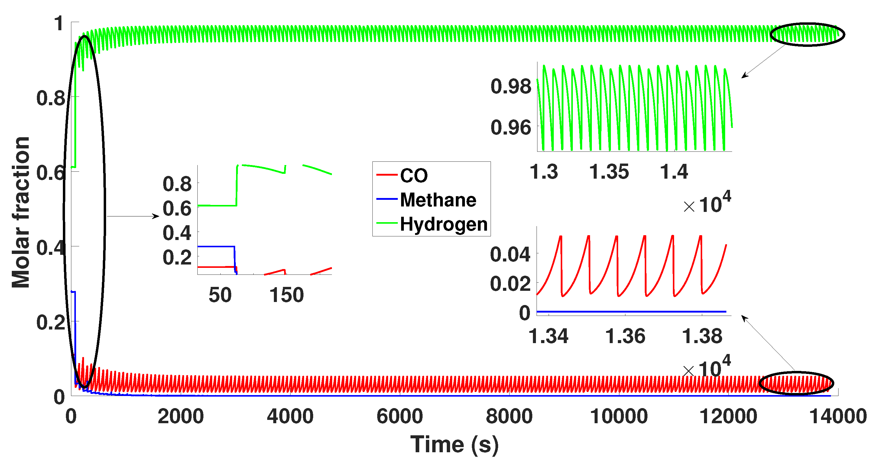
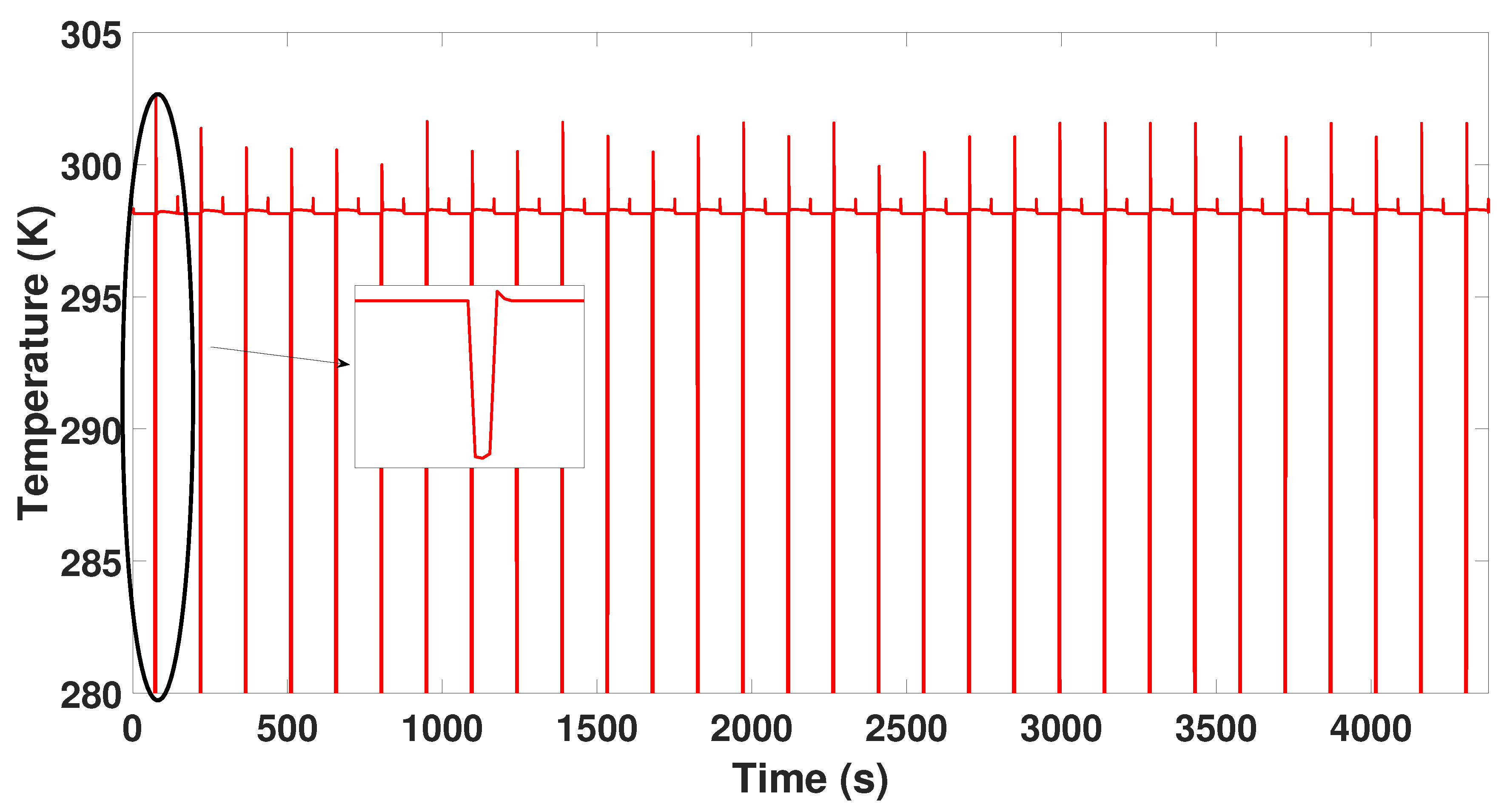
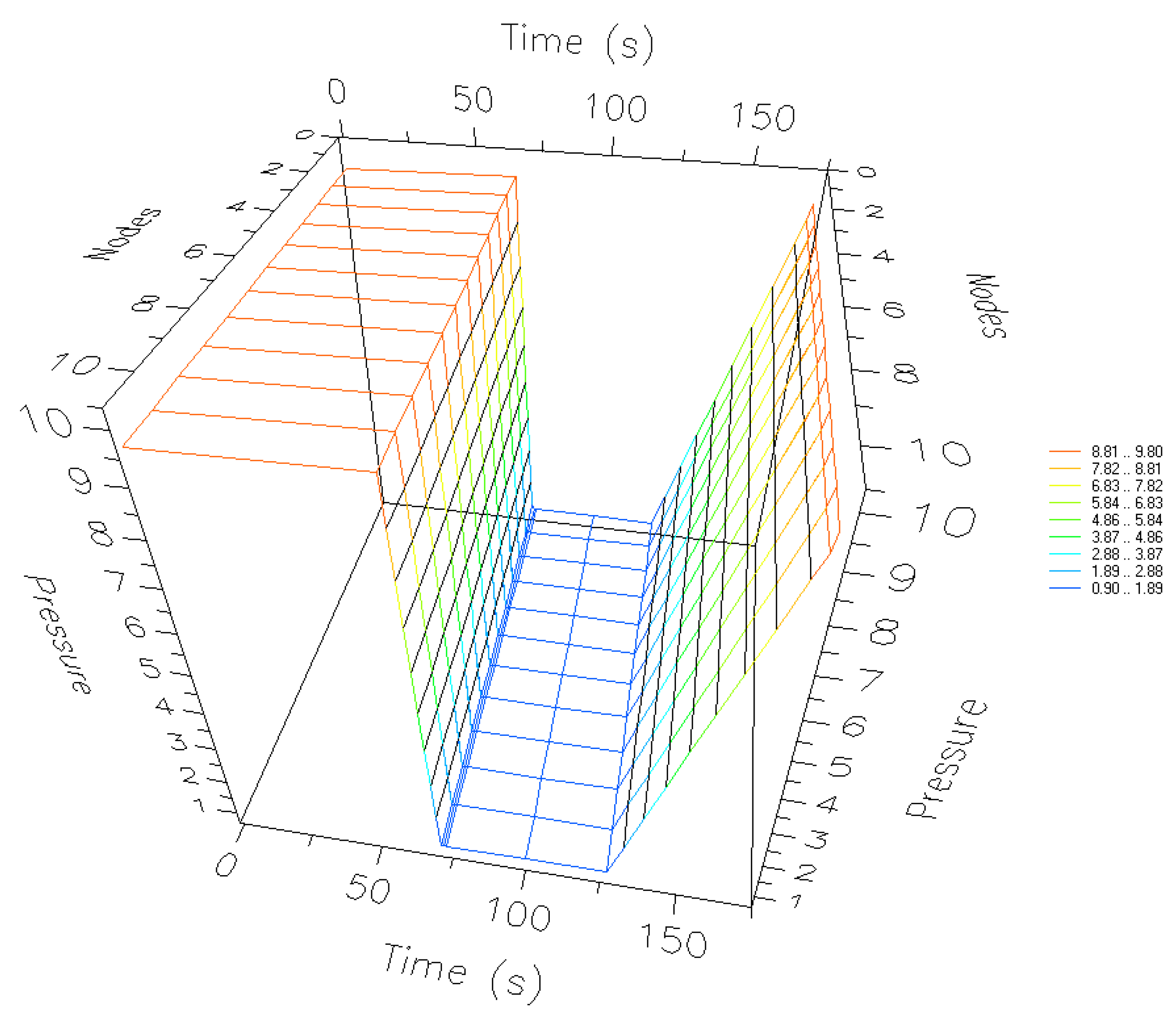
3. Simulation of the PSA Process for the Production of Bio-Hydrogen

The PSA process for the production of bio-hydrogen starts with nominal values established in

Table 3. Parameter values used for the PSA process.

Feed	Value
Molar fraction of carbon monoxide $y_{CO}$	0.11
Molar fraction of hydrogen $y_{H_2}$	0.61
Molar fraction of methane $y_{C{H}_4}$	0.28
Production Temperature $T_F$	298.15 K
Production pressure $P_F$	980,000 Pa
Purge pressure $P_F$	101,300 Pa
Bed length l	1 m
Bed Diamter D	0.037 m
Inter-particle ${ϵ}_i$	0.433
Intra-particle ${ϵ}_p$	0.347
Bulk solid density of adsorbent ${\rho }_p$	850 kg m−3
Constant mass transfer coefficients $\left(CO\right)$ $MTC$	0.15 s−1
Constant mass transfer coefficients $\left(H_2\right)$ $MTC$	0.7 s−1
Constant mass transfer coefficients $\left(C{H}_4\right)$ $MTC$	0.195 s−1
Adsorbent particle radius $r_p$	0.0015 m
Isotherm parameter ($I{P}_{1CO}$)	0.03385 $n/a$
Isotherm parameter ($I{P}_{1H_2}$)	0.01694$n/a$
Isotherm parameter ($I{P}_{1C{H}_4}$)	0.02386 $n/a$
Isotherm parameter ($I{P}_{2CO}$)	9.072 $\times {10}^{-5}$ $n/a$
Isotherm parameter ($I{P}_{2H_2}$)	2.1 $\times {10}^{-5}$  $n/a$
Isotherm parameter ($I{P}_{2C{H}_4}$)	5.621 $\times {10}^{-5}$  $n/a$
Isotherm parameter ($I{P}_{3CO}$)	2.311 $\times {10}^{-4}$ $n/a$
Isotherm parameter ($I{P}_{3H_2}$)	6.248 $\times {10}^{-5}$  $n/a$
Isotherm parameter ($I{P}_{3C{H}_4}$)	0.03478$n/a$
Isotherm parameter ($I{P}_{4CO}$)	1751.0 $n/a$
Isotherm parameter ($I{P}_{4H_2}$)	1229 $n/a$
Isotherm parameter ($I{P}_{4C{H}_4}$)	1159 $n/a$
Computational parameters
Number of nodes	10
Discretization method to be used	UDS1 first order (Derivatióntiny of Upwind Differencing Scheme 1)

. In Figure 3, it is possible to observe that the composition profiles ($H_{2}O$, $CO$, and $C{H}_4$) have oscillatory behavior, which is due to the nature of the PSA. The oscillatory dynamics generated with pressure changes allow to adsorb and desorb the water molecules on the surface of the type 5A zeolite. The hydrogen purity profile rises to a value of 0.99 in the molar fraction, while the other compounds decrease, which continues until reaching the CSS in a time of 1200 s.

In the case of the temperature profile from the start-up to the CSS, the behavior can be observed in Figure 4. This figure shows the oscillatory but stable behavior of the temperature, generating oscillating values between 300 K and 280 K, allowing favor for the adsorption and regeneration of the bed.

For hydrogen production, the four-step configuration is presented, shown in Figure 5. In the first 70 s of adsorption, a pressure of 980 kPa is carried out. Later, a depressurization is reached that causes the pressure to drop from 980 kPa to 15 kPa in a time of 3 s. Then, depressurization is achieved with a purge injected that goes from 15 kPa until reaching a pressure of 10 kPa in a time of 70 s. Finally, to finish one cycle, the repressurization goes from a purge pressure of 10 kPa until reaching 980 kPa again. These dynamics are repeated for the two beds interacting with the valves and steps configuration, as shown in Figure 1.

The pressure swing values for each step are shown in Figure 5 and the start times for each step are shown in Figure 1.

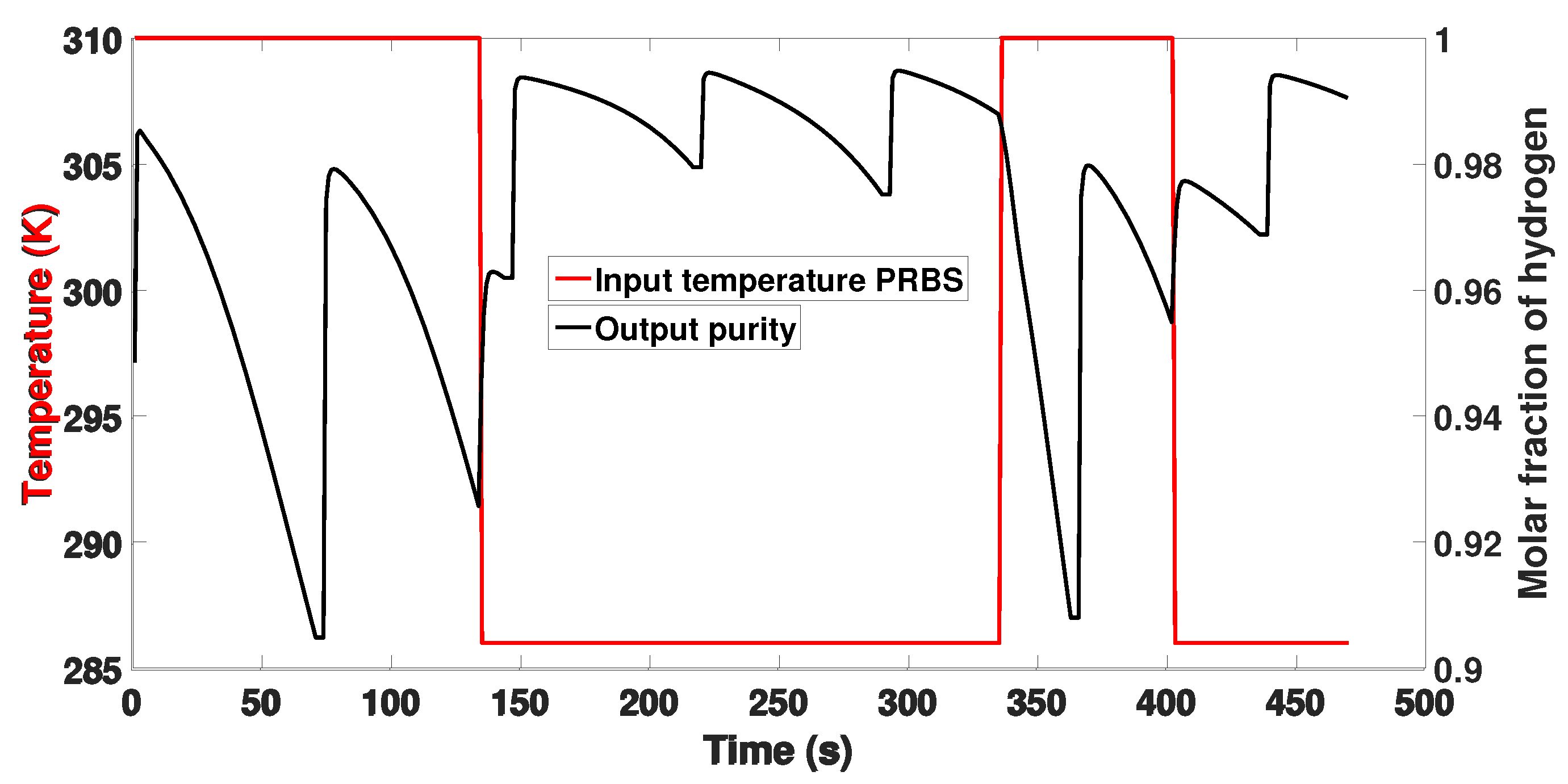
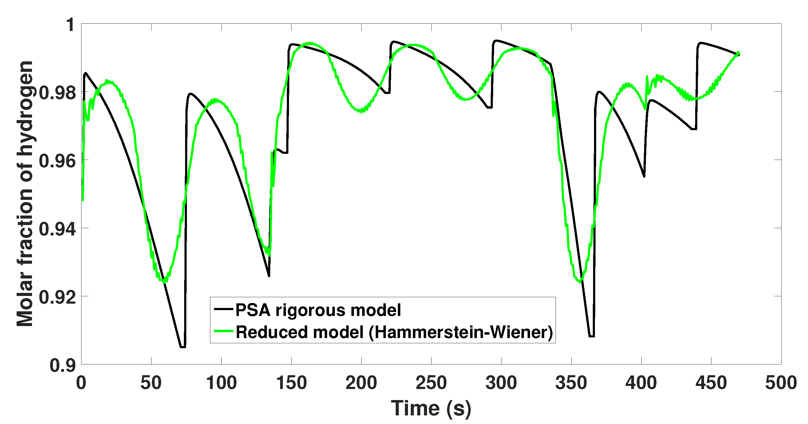
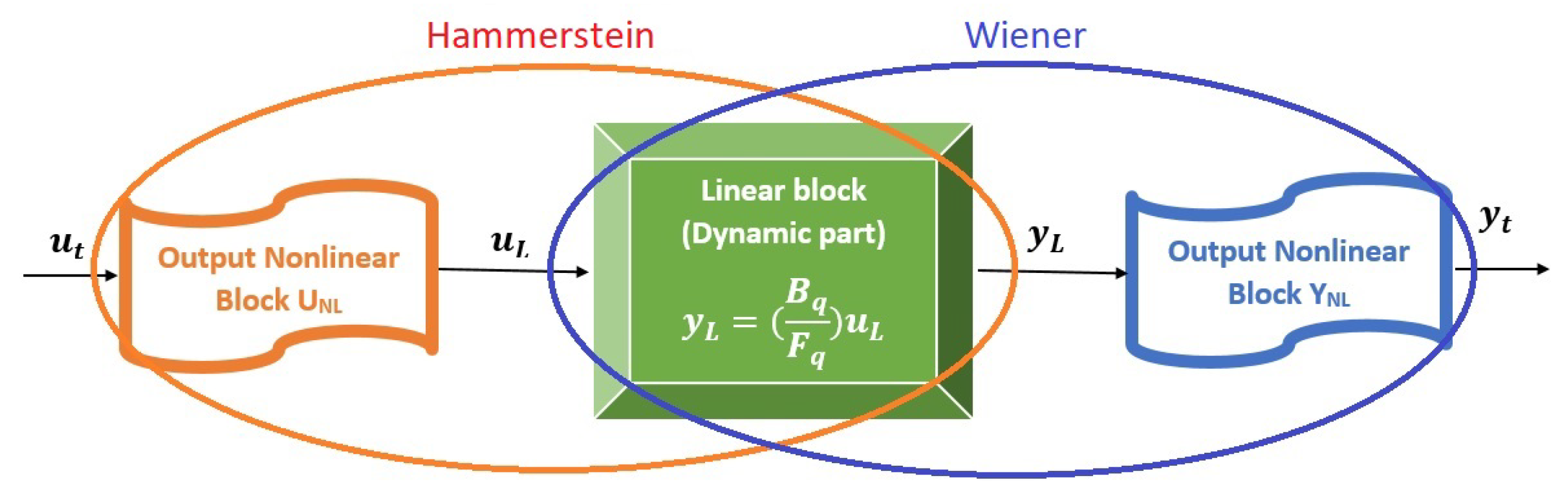
4. Identification of a Reduced Model

In order to design a robust controller capable of maintaining the PSA process stable even with the presence of actuator faults, it is necessary to obtain the input and output data of the rigorous PSA model, which are used to obtain an identified model, which will allow generating a behavior similar to that of the highly nonlinear model of the PSA process for the production of hydrogen.

To find an identified model, it was decided to use input and output data obtained from the rigorous PSA model. The temperature variable was defined as input, and the hydrogen purity was established as output (see Figure 6).

A 4-bit pseudo binary sequence (PRBS) was created; this PRBS allows reaching stability in a time of 300 s and a variation of ±0.5%. From these input data that were introduced in the plant PSA, the output with hydrogen purity data was generated using a sample time of 1 s.

The input and output data were used to find the reduced model by using the MatLab system identification toolbox. The identified model was a Hammerstein–Wiener. It can be seen in Figure 7 how the identified model captures the dynamics of the data acquired by the rigorous PSA model. This model has a fit of 87% over the real measurement of the PSA process.

The obtained Hammerstein–Wiener model is composed of three blocks, which can be seen in Figure 8. The blocks located at the input and output are non-linear blocks with static gains, while the center block is the dynamic part of the PSA process.

The FTC uses the linear block and the nonlinear input and output blocks with their inverse functions. Likewise, the continuous linear block is converted to a discrete state-space model in order to design discrete controllers. The overall structure can be seen in Figure 9.

The inverse functions of the non-linear static gain blocks for the input and output, are shown in the following Equations (6) and (7):

$$u_t=\left\{\begin{array}{cc}3.5u_L+305.2,\hfill & 49.993<u_L\le 50.844,\hfill \\ 2.6u_L+306.6,\hfill & 50.844<u_L\le 51.967,\hfill \\ 2.3u_L+307.7,\hfill & 51.967<u_L\le 53.238,\hfill \\ 2.3u_L+308.9,\hfill & 53.238<u_L\le 54.532,\hfill \\ 2.3u_L+309.1,\hfill & 54.532<u_L\le 55.724,\hfill \\ 3.0u_L+310.2,\hfill & 55.724<u_L\le 56.688.\hfill \end{array}\right.$$

(6)

$$y_L=\left\{\begin{array}{cc}0.012y_t-11.55,\hfill & 0.965<y_t\le 0.975,\hfill \\ 160.551y_t-182.08,\hfill & 0.975<y_t\le 0.991,\hfill \\ -539.807y_t+512.08,\hfill & 0.881<y_t\le 0.965,\hfill \\ -302.482y_t+302.76,\hfill & 0.766<y_t\le 0.881.\hfill \end{array}\right.$$

(7)

The continuous linear block is expressed as the following continuous state- space representation:

$$\begin{array}{cc}\hfill \dot{x}\left(t\right)& =Ax\left(t\right)+Bu\left(t\right),\hfill \\ \hfill y\left(t\right)& =Cx\left(t\right),\hfill \end{array}$$

(8)

with

$$\begin{array}{cc}\hfill A& =\left[\begin{array}{cccccccccc}2.930& -1.446& 0.504& 0.085& -0.334& 0.337& -0.124& 0.007& 0.039& -0.113\\ 2& 0& 0& 0& 0& 0& 0& 0& 0& 0\\ 0& 1& 0& 0& 0& 0& 0& 0& 0& 0\\ 0& 0& 1& 0& 0& 0& 0& 0& 0& 0\\ 0& 0& 0& 1& 0& 0& 0& 0& 0& 0\\ 0& 0& 0& 0& 1& 0& 0& 0& 0& 0\\ 0& 0& 0& 0& 0& 1& 0& 0& 0& 0\\ 0& 0& 0& 0& 0& 0& 1& 0& 0& 0\\ 0& 0& 0& 0& 0& 0& 0& 0.500& 0& 0\\ 0& 0& 0& 0& 0& 0& 0& 0& 0.250& 0\end{array}\right],\hfill \\ \hfill B& ={\left[\begin{array}{cccccccccc}1& 0& 0& 0& 0& 0& 0& 0& 0& 0\end{array}\right]}^{\top },\hfill \\ \hfill C& =\left[\begin{array}{cccccccccc}-0.340& 0.500& -0.490& 0.160& 0& 0& 0& 0& 0& 0\end{array}\right],\hfill \end{array}$$

where $A,B$ and C are matrices with the proper dimensions obtained with the identification process. The state vector is represented by $x\in {\mathbb{R}}^n$, $u\in {\mathbb{R}}^m$ is the input of control vector, $y\in {\mathbb{R}}^p$ represents the system outputs, and t is the time variable. After obtaining the inverse functions and the continuous model, the following section presents the design of the discrete controller by using the Hammerstein–Wiener structure.

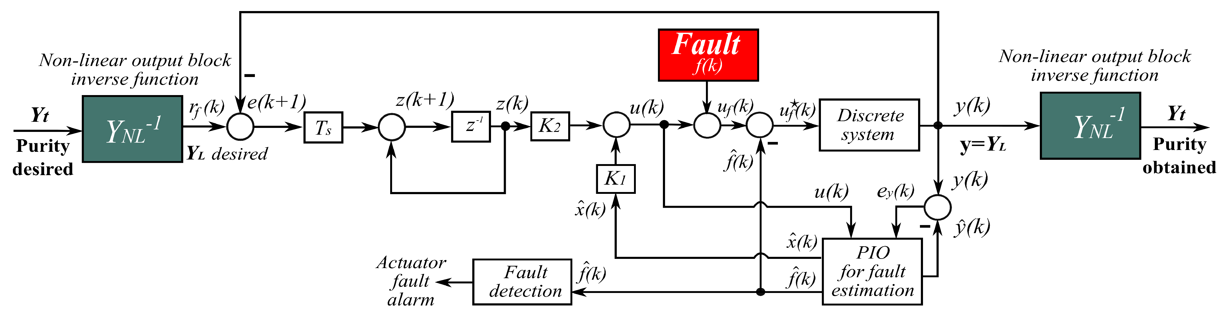
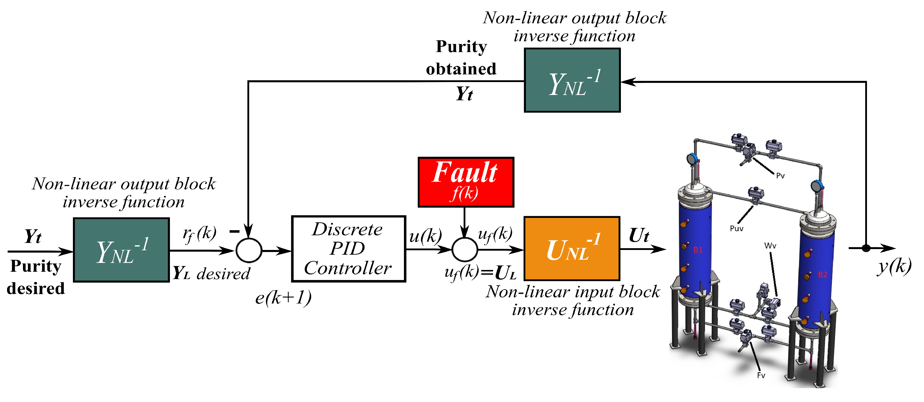
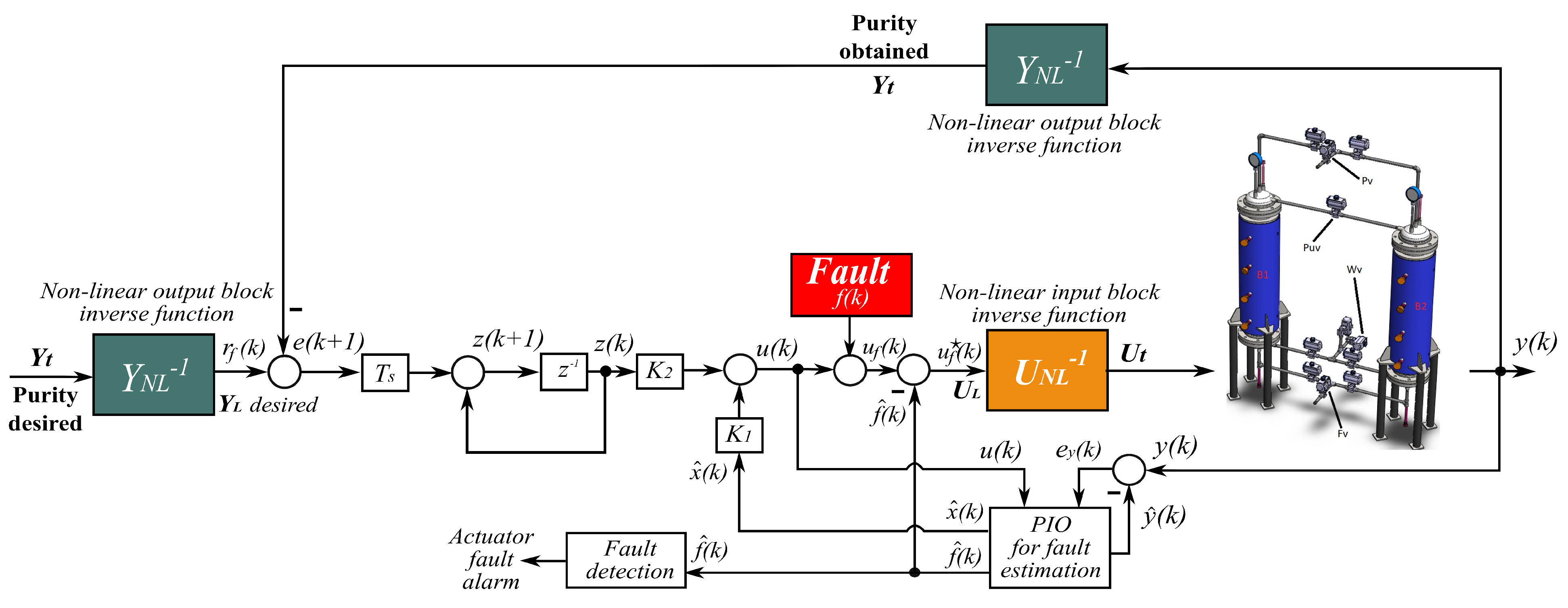
5. Active Fault-Tolerant Controller Design

In this section, the discrete FTC (fault-tolerant control) design is applied to the PSA process with actuator faults (see Figure 10). First, the nominal discrete controller is presented. Secondly, the FDD (fault detection and diagnosis) system is developed in order to detect, estimate and isolate the actuator faults. Finally, the FTC scheme is presented by showing the fault-accommodation performance.

5.1. Nominal Discrete Controller

The feedback control law is designed such that the steady-state response tends to the desired reference signal $r_f\left(k\right)$. The continuous system (8) is rewritten in a discrete form by using the Euler method, as follows:

$$\begin{array}{cc}\hfill x(k+1)& =A_{d}x\left(k\right)+B_{d}u\left(k\right),\hfill \\ \hfill y\left(k\right)& =C_{d}x\left(k\right),\hfill \end{array}$$

(9)

where $A_d,B_d$ and $C_d$ are matrices with proper dimensions. The error is expressed as $e\left(k\right)=r_f\left(k\right)-C_{d}x\left(k\right)$, and the error dynamics can be formulated as

$$\begin{array}{cc}\hfill z(k+1)& =z\left(k\right)+T_s\left(e\left(k\right)\right)\hfill \\ \hfill & =z\left(k\right)+T_s\left(r_f\left(k\right)-C_{d}x\left(k\right)\right),\hfill \end{array}$$

(10)

where $z\left(k\right)$ is an auxiliary variable for integral control design, and $T_s$ is the sample time. By using (9) and (10), then $\overline{x}\left(k\right)={[x\left(k\right),z\left(k\right)]}^{\top }$ is an augmented system that can be expressed as follows:

$$\begin{array}{cc}\hfill \overline{x}(k+1)& ={\overline{A}}_c\overline{x}\left(k\right)+{\overline{B}}_{c}u\left(k\right)+{\overline{R}}_c{r}_f\left(k\right),\hfill \\ \hfill \overline{y}\left(k\right)& ={\overline{C}}_c\overline{x}\left(k\right),\hfill \end{array}$$

(11)

with

$$\begin{array}{cc}\hfill {\overline{A}}_c& =\left[\begin{array}{cc}{A}_d& 0\\ -C_d{T}_s& 1\end{array}\right],{\overline{B}}_c=\left[\begin{array}{c}{B}_d\\ 0\end{array}\right],\hfill \\ \hfill {\overline{C}}_c& =\left[\begin{array}{cc}{C}_d& 0\end{array}\right],{\overline{R}}_c=\left[\begin{array}{c}0\\ T_s\end{array}\right].\hfill \end{array}$$

Then, the nominal control law $u\left(k\right)$ is defined by

$$\begin{array}{cc}\hfill u\left(k\right)& =-{\overline{K}}_c\overline{x}\left(k\right)=-\left[\begin{array}{cc}{K}_1& K_2\end{array}\right]\left[\begin{array}{c}x\left(k\right)\\ z\left(k\right)\end{array}\right],\hfill \end{array}$$

(12)

where $K_1$ and $K_2$ are the state feedback gains. Then, the following closed-loop system can be obtained, by using (12) in the system (11), as follows:

$$\begin{array}{cc}\hfill \overline{x}(k+1)& =({\overline{A}}_c+{\overline{B}}_c{\overline{K}}_c)\overline{x}\left(k\right).\hfill \end{array}$$

(13)

Given (11) and the control law (12), the close-loop error system (10) is asymptotically stable if there exist a symmetric matrix $X=X^{\top }>0$ and a matrix W such that

$$\begin{array}{c}\hfill \left[\begin{array}{cc}X& {\overline{A}}_{c}X+{\overline{B}}_{c}W\\ {({\overline{A}}_{c}X+{\overline{B}}_{c}W)}^{\top }& X\end{array}\right]>0.\end{array}$$

(14)

The controller gain is calculated by using ${\overline{K}}_c=W{X}^{-1}$. The proof is presented in [37]. Additionally, in order to avoid slow dynamics, the pole assignment can be considered as

$$\begin{array}{c}\hfill {\lambda }_i({\overline{A}}_c-{\overline{B}}_c{\overline{K}}_c)\in \mathbb{D},i=1,2,\cdots ,n,\end{array}$$

(15)

where the disk stability is defined by $\mathbb{D}$ with all the eigenvalues of $({\overline{A}}_c-{\overline{B}}_c{\overline{K}}_c)$ located inside the unit circle, as defined in [37,38]. Thus, given (15), (11) and the control law (12), the closed-loop error system (10) is asymptotically stable if there exists a positive scalar r, a symmetric matrix $X=X^{\top }>0$ and a matrix W such that

$$\begin{array}{c}\hfill \left[\begin{array}{cc}-rX& {\overline{A}}_{c}X+{\overline{B}}_{c}W\\ {({\overline{A}}_{c}X+{\overline{B}}_{c}W)}^{\top }& -rX\end{array}\right]<0.\end{array}$$

(16)

Finally, the nominal controller gain matrix is computed by ${\overline{K}}_c=W{X}^{-1}$.

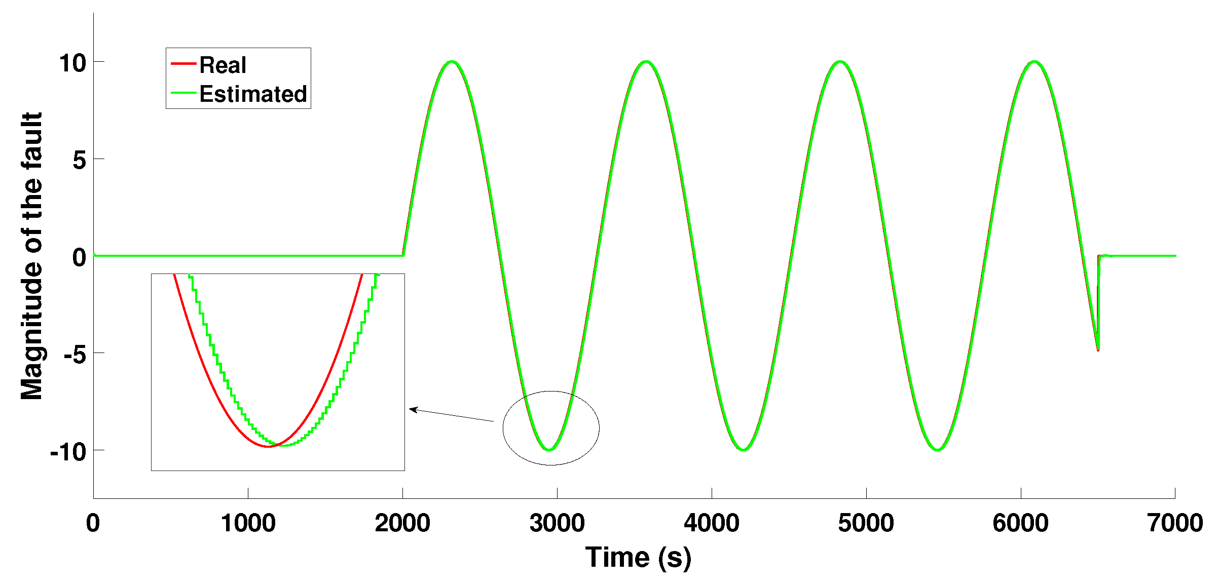
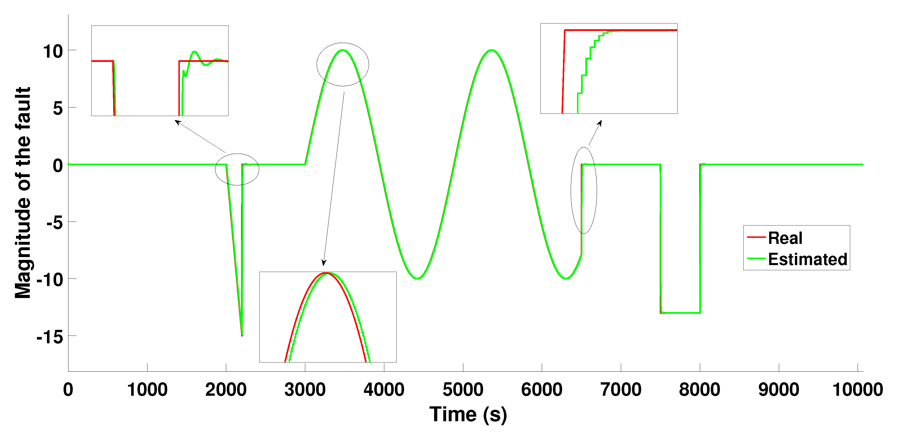
5.2. Fault Detection and Diagnosis System

A discrete proportional–integral observer (PIO) is used to achieve the proposed FDD strategy. System (9) with an actuator additive fault signal $f\left(k\right)$ can be rewritten in the augmented faulty discrete linear form $x_a\left(k\right)={[x\left(k\right),f\left(k\right)]}^{\top }$, as follows:

$$\begin{array}{cc}\hfill x_a(k+1)& =A_a{x}_a\left(k\right)+B_{a}u\left(k\right),\hfill \\ \hfill y_a\left(k\right)& =C_a{x}_a\left(k\right),\hfill \end{array}$$

(17)

with

$$\begin{array}{cc}\hfill A_a& =\left[\begin{array}{cc}{A}_d& B_d\\ 0& 1\end{array}\right],B_a=\left[\begin{array}{c}{B}_d\\ 0\end{array}\right],\hfill \\ \hfill C_a& =\left[\begin{array}{cc}{C}_d& 0\end{array}\right],\hfill \end{array}$$

where the actuator fault $f\left(k\right)$ is considered slow dynamics, that is, $f(k+1)=f\left(k\right)$. Now, a discrete PIO can be rewritten in the following augmented form ${\widehat{x}}_a\left(k\right)={[\widehat{x}\left(k\right),\widehat{f}\left(k\right)]}^{\top }$:

$$\begin{array}{cc}\hfill {\widehat{x}}_a(k+1)& =A_a{\widehat{x}}_a\left(k\right)+B_{a}u\left(k\right)+L_{PI}{e}_y\left(k\right),\hfill \\ \hfill {\widehat{y}}_a\left(k\right)& =C_a{\widehat{x}}_a\left(k\right),\hfill \end{array}$$

(18)

where $e_y\left(k\right)=y_a\left(k\right)-{\widehat{y}}_a\left(k\right)$ is the estimation error vector and $L_{PI}$ represents the observer gain. By using (17) and (18), the dynamics of the state estimation error $e_a\left(k\right)=x_a\left(k\right)-{\widehat{x}}_a\left(k\right)$ is represented by

$$\begin{array}{cc}\hfill e_a(k+1)& =(A_a-L_{PI}{C}_a)e_a\left(k\right).\hfill \end{array}$$

(19)

If the pair $(A_a,C_a)$ is completely observable, then an observer gain matrix $L_{PI}$ can be designed, and the eigenvalues of $(A_a-L_{PI}{C}_a)$ can be located inside the unit circle.

The real actuator fault detection is achieved at any time by using the actuator additive fault estimation signal $\widehat{f}\left(k\right)$. If $|\widehat{f}\left(k\right)|$ is close to zero, then the system is in a fault-free case, while if the absolute fault estimated value has a greater value than a defined threshold, then the system is in a fault case, activating an alarm indicator.

5.3. Fault Accommodation Control Law

If the fault is detected and estimated correctly, then a new control law is added to the nominal control law in order to accommodate the fault and reduce its effect on the system. The proposed fault accommodation control law is given by

$$\begin{array}{c}\hfill u_f^{*}\left(k\right)=u\left(k\right)-\widehat{f}\left(k\right),\end{array}$$

(20)

where the first part of the accommodation control law (20) is the faulty input signal, and the second part of the equation is the additive fault estimation to be added in order to accommodate the fault, as it is shown in Figure 10.

6. Results and Discussion

To evaluate the performance and robustness of the proposed active FTC, it is necessary to submit it to different tests. Additionally, we propose a comparison between the FTC scheme and a discrete PID controller. The gains of the discrete PID controller were tuned with the Ziegler–Nichols method. For the following tests, the controllers were implemented both in the reduced model and the rigorous PSA model.

The robustness of the controllers is evaluated by subjecting them to trajectory changes with different types of faults. These faults are classified as: intermittent, abrupt, and incipient. Two scenarios were considered in order to evaluate the performance of the controllers:

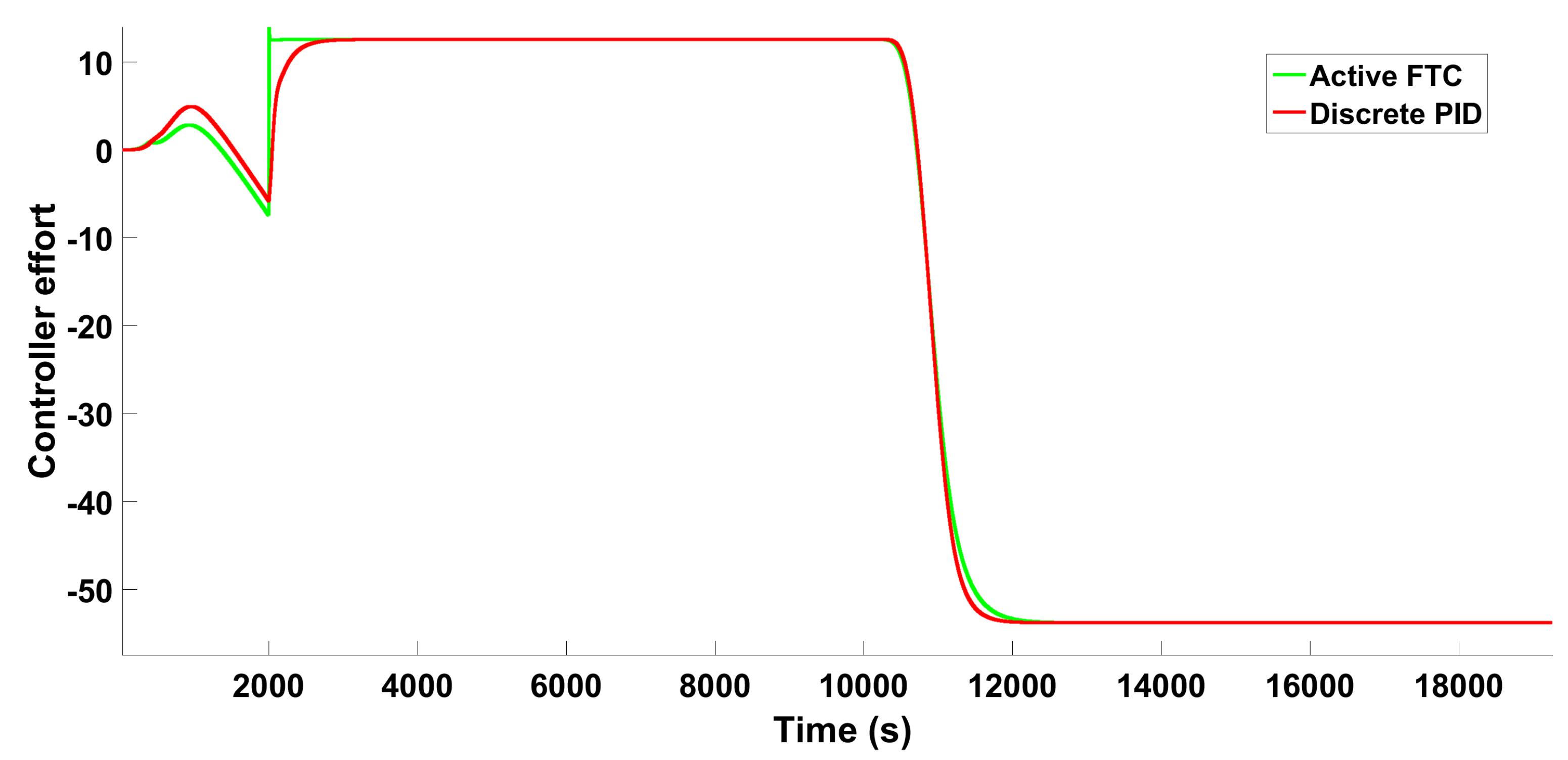
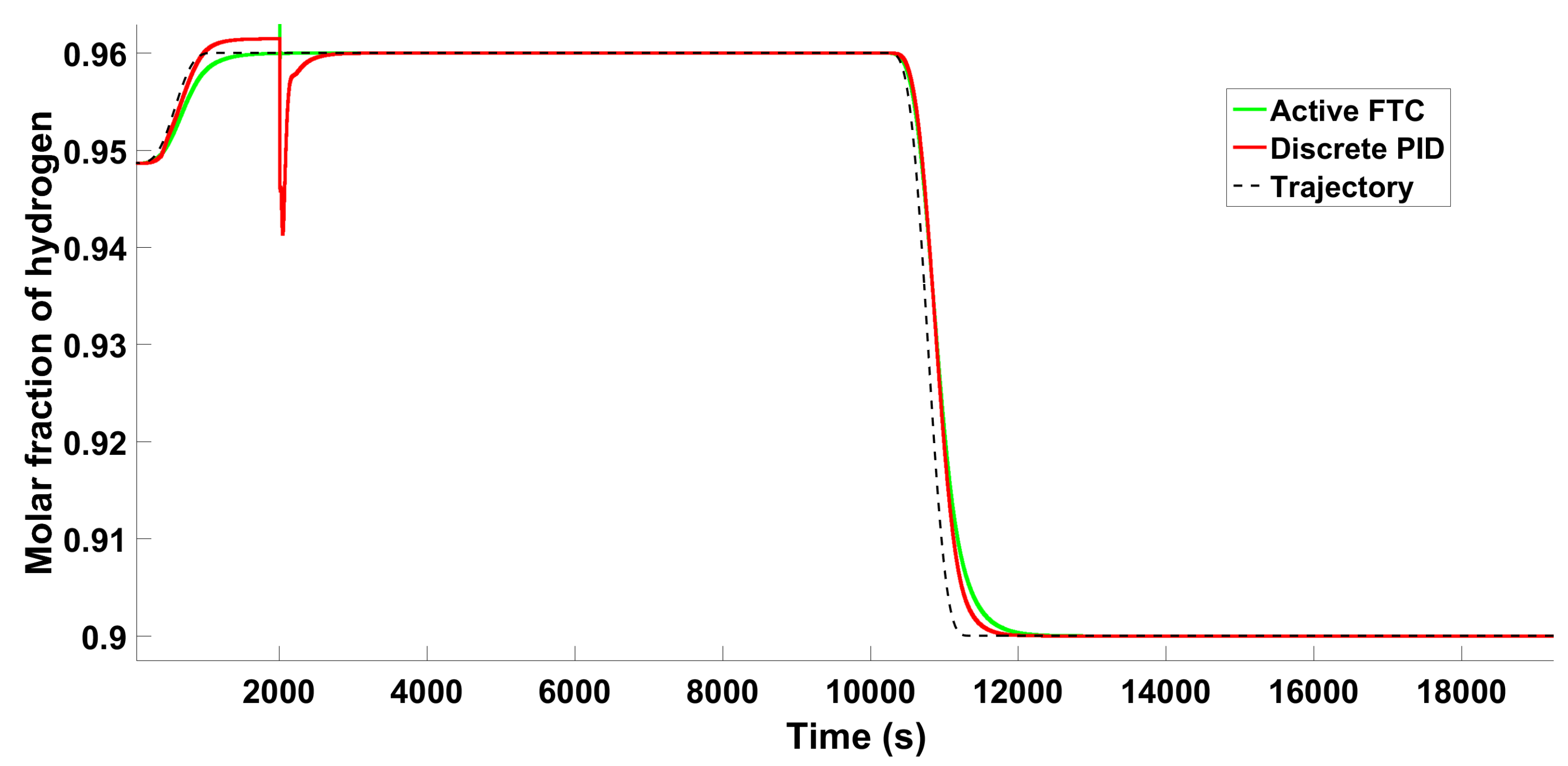
6.1. Scenario 1: Comparison between FTC and Discrete PID Controller on the Hammerstein–Wiener Model

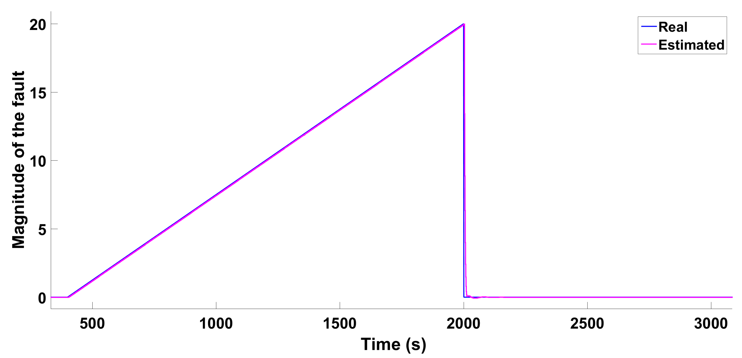
6.1.1. Scenario 1—Ramp-Type Fault

This first scenario is validated by using the scheme presented in Figure 10. For this scenario, a ramp-type fault is injected in the actuator at time 400 s with a magnitude of 20, represented by the following equation:

$$f_1\left(t\right)=\left\{\begin{array}{cc}0,\hfill & t<400s,\hfill \\ \left((t/400)-1\right)20,\hfill & 400s\le t\le 2000s.\hfill \end{array}\right.$$

(21)

This event is presented as a transient fault because it implies a temporary malfunction of the component. A transient fault is usually caused by energy fluctuations or magnetic radiation. The ramp-type fault appears as a constant loss of effectiveness with drift or calibration error, being considered an incipient fault. Figure 11 shows the real and estimation actuator fault, injected on the actuator of the reduced model system.

The control signals are depicted in Figure 12. It can be observed that, when the ramp-type fault is injected, the active FTC generates more input effort in order to compensate for the fault, compared to the discrete PID controller. Additionally, the hydrogen purity decreases more using the discrete PID in comparison with the proposed active FTC system (see Figure 13).

A comparison between the discrete PID controller and the proposed FTC applied to the faulty reduced model (Hammerstein–Wiener) is presented in Figure 13. Both controllers track correctly the desired purity trajectory. Clearly, the proposed strategy is robust with respect to the actuator fault. Even in the presence of a ramp-type fault, the proposed scheme follows the reference correctly.

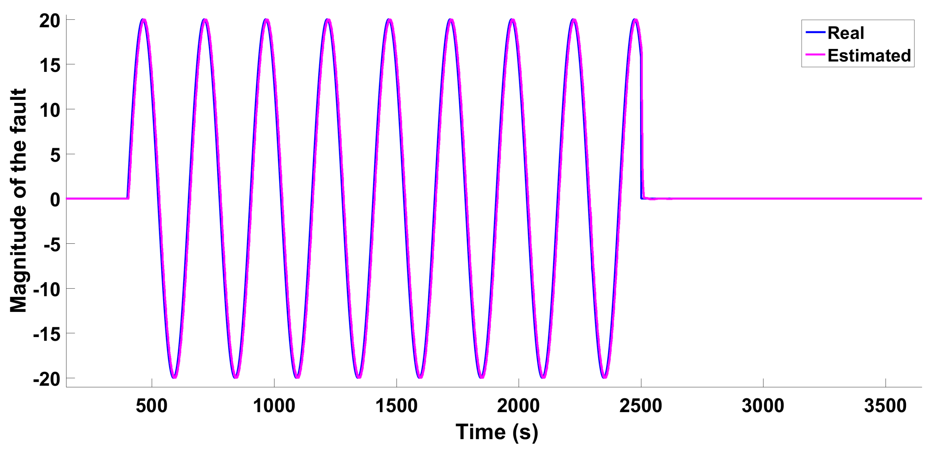
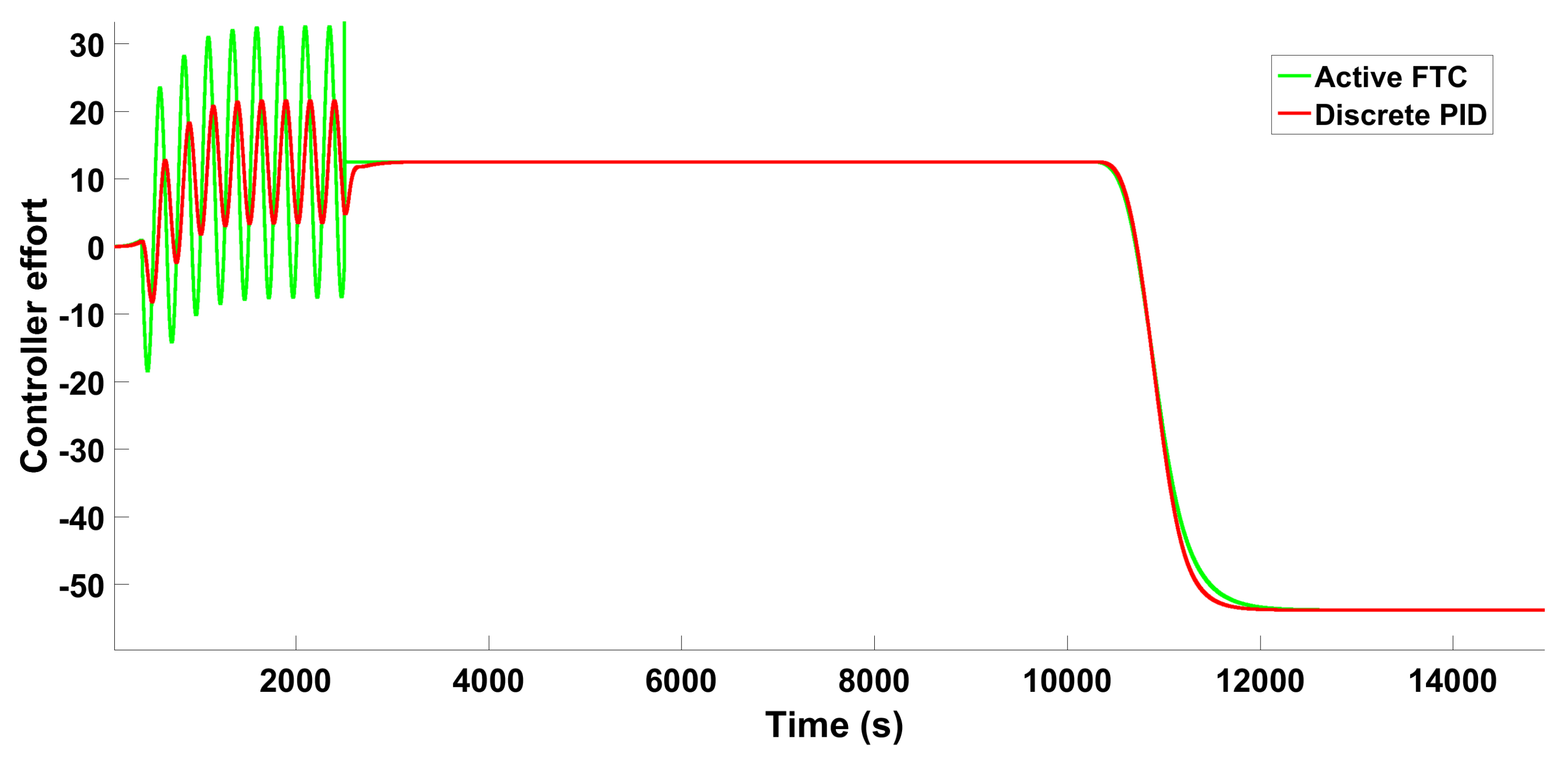
6.1.2. Scenario 1—Sine Wave-Type Fault

For this scenario, a sine wave-type fault is injected in the actuator at 400 s with a magnitude from 20 to −20. The sine wave-type fault is expressed with the following equation:

$$f_2\left(t\right)=\left\{\begin{array}{cc}0,\hfill & t<400s,\hfill \\ \sin \left((t/400)-1\right)20,\hfill & 400s\le t\le 2500s.\hfill \end{array}\right.$$

(22)

The sine wave type fault is handled as a transient and abrupt fault, which is applied to the actuator and appears as mechanical wear. Figure 14 shows the magnitude of the real fault and its estimation.

The control signals applied on the reduced model are presented in Figure 15. It can be seen that both controllers have an oscillatory behavior in their control signal, and this is due to the sine wave-type fault. The control signal generated with the active FTC is greater compared to the discrete PID. The input effort produced with the FTC signal has a range value between 30 and −10 in order to compensate for the actuator fault. Additionally, the active FTC reduces the effect of this type of oscillatory fault that can abruptly affect the real process (see Figure 16).

In Figure 16, a comparison between the faulty reduced model with the discrete PID and the FTC using the fault estimation generated by the PIO is displayed. Note that the error between the desired and the real hydrogen purity is bigger when the discrete PID is applied, with purities between 0.98 and 0.03 in the molar fraction. In addition, the active FTC is able to track correctly the hydrogen purity, even when an actuator sine wave-type fault is injected.

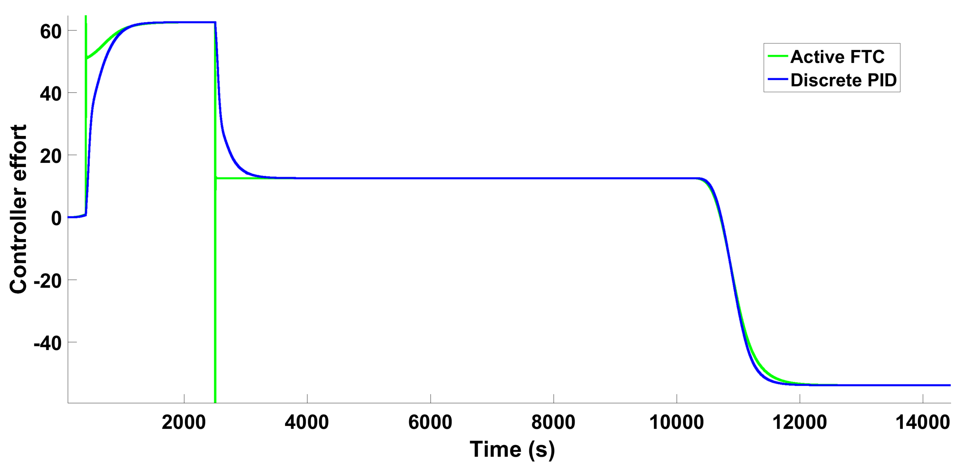
6.1.3. Scenario 1—Step-Type Fault

Subsequently, a third constant step-type fault is injected into the reduced model as an abrupt actuator additive fault. This type of fault occurs in time 400 s with a magnitude of −50, represented by the following equation:

$$f_3\left(t\right)=\left\{\begin{array}{cc}0,\hfill & t<400s,\hfill \\ -50,\hfill & 400s\le t\le 2500s.\hfill \end{array}\right.$$

(23)

This type of fault can be considered as a degradation of the actuator gain (constant loss of effectiveness); this is generated due to the deterioration of the material or a component fault. Figure 17 shows the real and estimated step-type fault applied to the reduced model.

The control signals are presented in Figure 18. When the step-type fault is injected, the FTC produces more control effort in order to compensate for the fault. Additionally, the hydrogen purity decreases to 0.9 in the molar fraction when the discrete PID strategy is used in comparison with the FTC system (see Figure 19).

In Figure 19, a comparison between the faulty Hammerstein–Wiener model with the discrete PID controller and the FTC is displayed. From this figure, note that the error between the desired and the real hydrogen purity is bigger when the discrete FTC is not applied. Additionally, the active FTC scheme is able to track correctly the hydrogen purity, even when an actuator step-type fault occurs, with a smaller error compared with the discrete PID controller.

6.2. Scenario 2: Comparison between FTC and Discrete PID Controller on the PSA Process

6.2.1. Scenario 2—Nominal Controllers for the Following Trajectory

In the second scenario, the robustness and tracking performance of the controllers are evaluated by injecting actuator faults and changes in purity, respectively, applied to the rigorous PSA model (virtual plant). To implement the controllers in the rigorous PSA model, it was necessary to use the inverse functions, represented by Equations (6) and (7). The control schemes for each controller are presented in Figure 20 and Figure 21.

For the first part of the second scenario, we analyze a comparison between the FTC scheme and the discrete PID by using the nominal controllers without faults by considering only tracking the desired purity trajectory. The trajectory follow-up test was carried out to achieve purities of 0.9999 molar fraction (99.99%). The results obtained are shown in Figure 22.

It can be seen in Figure 22 the control signals generated by the controllers and the purity dynamics with two trajectory changes. The discrete PID control generates a signal similar to the active FTC; however, it can be seen that the active FTC signal has a faster response than the discrete PID. This means that the purity obtained by the active FTC has better results, obtaining a higher purity and with smaller oscillations compared to those obtained with the discrete PID.

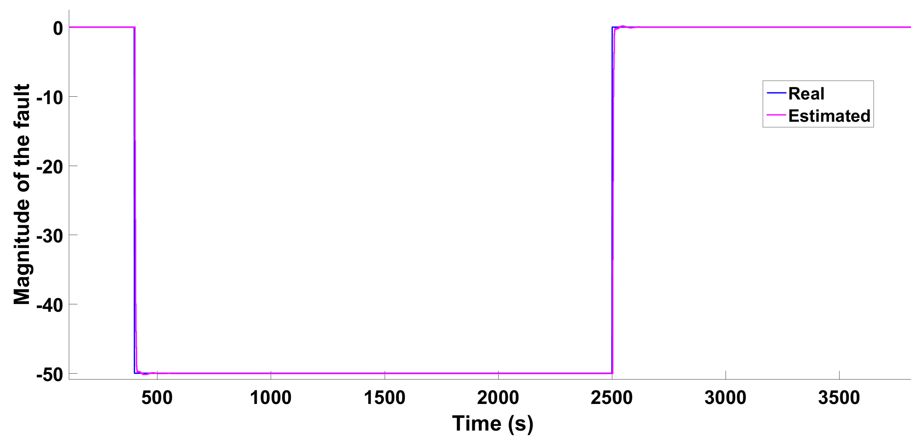
6.2.2. Scenario 2—Individual Fault

For the second part of the second scenario, an individual sine wave-type fault is injected into the actuator of the PSA virtual plant. This fault is considered a constant loss of effectiveness and could be seen as actuator gain degradation due to material aging or component fault. This type of fault is an intermittent, non-constant variable (sine wave), and it is injected at time 2000 s with an oscillatory magnitude between 10 and −10, represented by the following equation:

$$f_4\left(t\right)=\left\{\begin{array}{cc}0,\hfill & 2000\le t\le 6500s,\hfill \\ \sin \left((t/2000)-1\right)20,\hfill & t\ge 2000s.\hfill \end{array}\right.$$

(24)

Figure 23 shows the real and estimated individual sine wave-type fault applied to the actuator of the PSA virtual plant. It can be seen that the fault estimation algorithm is adequate to reproduce the magnitude and time that a sine wave-type fault occurs.

Figure 24 shows the control signals generated by the active FTC and discrete PID, as well as the purity results. It is possible to observe that the discrete PID tends to have an oscillatory dynamic in its control signal and this consequently generates intermittent decreases in the obtained purity. On the other hand, the active FTC reduces the error between the desired and the real hydrogen purity. The discrete PID controller does not achieve maintenance of the desired purity, and this means that it cannot meet international standards for use as bio-fuel.

6.2.3. Scenario 2−Multiple Faults

Finally, a robust test was carried out with three types of faults: two abrupt additive faults, and the sine wave-type fault. The presence of the three different faults is considered an intermittent fault because there are repeated occurrences of transient faults, and it could be due to, for example, loose cables.

It can be seen that each fault scenario provides useful information on the effectiveness and performance of the controllers, and each of them corresponds to a different type of actuator fault that can occur in the PSA plant. The consequences of this type of fault in the PSA process can result in a product concentration or purity lower than that which meets international purity standards, or even catastrophic dynamics can occur. The three faults are represented by the following equation:

$$f_5\left(t\right)=\{\begin{array}{cc}0,\hfill & t<2000s,\hfill \\ \left(\right(t/2000)-1)\ast 100,\hfill & 2000s\le t\le 2100s,\hfill \\ 0,\hfill & 3000\le t\le 6500s,\hfill \\ 20\sin (t/3000)-1,\hfill & t\ge 3000s,\hfill \\ 0,\hfill & t<7500s,\hfill \\ -50,\hfill & 7500s\le t\le 8000s.\hfill \end{array}$$

(25)

.

Figure 25 shows the real and estimated multiple faults injected on the PSA virtual plant. This figure shows a correct estimation of the ramp, sine, and step-type faults.

A comparison between the control signals generated by the active FTC and the discrete PID controller is presented in Figure 26. The signals generated by the discrete PID are smooth but with an oscillating tendency when the sine wave-type fault is injected. Likewise, a greater control effort is observed when the step-type fault occurs, generating temperatures between 310 K and 275 K. The active FTC has less effort on sine wave and step faults, quickly exceeding the effort generated to maintain the PSA process stable and reduce the fault effect.

Additionally, Figure 26 shows the results obtained in the presence of three faults and a reference change. The active FTC has better performance and robustness by following the desired purity, while the discrete PID presents a bigger error between the desired and the real hydrogen purity, obtaining values that do not meet international standards to be used as bio-fuel.

The proposed active fault-tolerant control is superior to the discrete PID controller because the method uses a fault detection and diagnosis system and accommodation strategy. The fault detection and diagnosis system is developed with a proportional–integral observer that can estimate ramp, sine wave, and step non-constant faults. This actuator fault estimation is compared with a predefined threshold to perform fault detection. Finally, when the fault is detected correctly then the fault estimation signal is added to the nominal controller to compensate for the effect of the non-constant faults.

7. Conclusions

In this work, the analysis and validation of two controllers that achieve maintenance of the PSA process stable for the production of bio-hydrogen were presented. It was observed that the discrete PID controller performs well in following trajectory changes. Furthermore, the controller does not generate the necessary effort to quickly reach the desired purity and tends to have large purity oscillating ranges, which are not suitable to produce bio-hydrogen with a high degree of purity. Likewise, the discrete PID controller does not have a fast response to generate the effort necessary to reduce the effect of certain faults. The purity results obtained with the discrete PID controller before the actuator faults are values of 0.94, 0.93, and 0.92 in molar fraction.

On the other hand, the proposed active FTC is robust with respect to actuator faults and mitigates its effects in comparison to the discrete PID controller. The active FTC presents great results since in all cases it achieves maintenance of the PSA process stability and achieves compliance with international purity standards to be used as bio-fuel. The hydrogen purity obtained with the FTC has values of 0.98 and 0.99 in the molar fraction, even with changes in the desired trajectory and with actuator faults.

It is important to mention that the active FTC input signal results are greater than the discrete PID ones. This can allow the values over the temperature to be exceeded, and consequently, an input saturation can occur by reaching the limit of the effort allowed by the handled temperatures. Therefore, it is important to consider the maximum and minimum limits (restrictions) on the active FTC scheme.

For future work, it is very important to make a comparison between the active FTC with other controllers, such as an optimal model predictive control (MPC), in order to verify the efficiency in the production and recovery of bio-hydrogen. Additionally, experimental results will be carried out.

References

1. Guan, Z.; Wang, Y.; Yu, X.; Shen, Y.; He, D.; Tang, Z.; Li, W.; Zhang, D. Simulation and analysis of dual-reflux pressure swing adsorption using silica gel for blue coal gas initial separation. Int. J. Hydrogen Energy 2021, 46, 683–696. [Google Scholar] [CrossRef]
2. Chicano, J.; Dion, C.T.; Pasaogullari, U.; Valla, J.A. Simulation of 12-bed vacuum pressure-swing adsorption for hydrogen separation from methanol-steam reforming off-gas. Int. J. Hydrogen Energy 2021, 46, 28626–28640. [Google Scholar] [CrossRef]
3. Zhang, N.; Xiao, J.; Bénard, P.; Chahine, R. Single- and double-bed pressure swing adsorption processes for H2/CO syngas separation. Int. J. Hydrogen Energy 2019, 44, 26405–26418. [Google Scholar] [CrossRef]
4. Delgado Dobladez, J.A.; Águeda Maté, V.I.; Torrellas, S.Á.; Larriba, M.; Brea, P. Efficient recovery of syngas from dry methane reforming product by a dual pressure swing adsorption process. Int. J. Hydrogen Energy 2021, 46, 17522–17533. [Google Scholar] [CrossRef]
5. Fakhroleslam, M.; Bozorgmehry Boozarjomehry, R.; Fatemi, S. Design of a dynamical hybrid observer for pressure swing adsorption processes. Int. J. Hydrogen Energy 2017, 42, 21027–21039. [Google Scholar] [CrossRef]
6. Du, Z.; Liu, C.; Zhai, J.; Guo, X.; Xiong, Y.; Su, W.; He, G. A Review of Hydrogen Purification Technologies for Fuel Cell Vehicles. Catalysts 2021, 11, 393. [Google Scholar] [CrossRef]
7. Zhang, R.; Shen, Y.; Tang, Z.; Li, W.; Zhang, D.A.; Raganati, F.; Zhang, R.; Shen, Y.; Tang, Z.; Li, W.; et al. A Review of Numerical Research on the Pressure Swing Adsorption Process. Processes 2022, 10, 812. [Google Scholar] [CrossRef]
8. Luberti, M.; Ahn, H. Review of Polybed pressure swing adsorption for hydrogen purification. Int. J. Hydrogen Energy 2022, 47, 10911–10933. [Google Scholar] [CrossRef]
9. Zhang, X.; Bao, C.; Zhou, F.; Lai, N.C. Modeling study on a two-stage hydrogen purification process of pressure swing adsorption and carbon monoxide selective methanation for proton exchange membrane fuel cells. Int. J. Hydrogen Energy 2023. [Google Scholar] [CrossRef]
10. Di Marcoberardino, G.; Vitali, D.; Spinelli, F.; Binotti, M.; Manzolini, G. Green Hydrogen Production from Raw Biogas: A Techno-Economic Investigation of Conventional Processes Using Pressure Swing Adsorption Unit. Processes 2018, 6, 19. [Google Scholar] [CrossRef] [Green Version]
11. Garcia, R.; Gómez-Díaz, D.; Kalman, V.; Voigt, J.; Jordan, C.; Harasek, M. Hydrogen Purification by Pressure Swing Adsorption: High-Pressure PSA Performance in Recovery from Seasonal Storage. Sustainability 2022, 14, 14037. [Google Scholar] [CrossRef]
12. Zhang, N.; Bénard, P.; Chahine, R.; Yang, T.; Xiao, J. Optimization of pressure swing adsorption for hydrogen purification based on Box-Behnken design method. Int. J. Hydrogen Energy 2021, 46, 5403–5417. [Google Scholar] [CrossRef]
13. Vo, N.D.; Oh, D.H.; Kang, J.H.; Oh, M.; Lee, C.H. Dynamic-model-based artificial neural network for H2 recovery and CO2 capture from hydrogen tail gas. Appl. Energy 2020, 273, 115263. [Google Scholar] [CrossRef]
14. López Núñez, A.R.; Rumbo Morales, J.Y.; Salas Villalobos, A.U.; De La Cruz-Soto, J.; Ortiz Torres, G.; Rodríguez Cerda, J.C.; Calixto-Rodriguez, M.; Brizuela Mendoza, J.A.; Aguilar Molina, Y.; Zatarain Durán, O.A.; et al. Optimization and Recovery of a Pressure Swing Adsorption Process for the Purification and Production of Bioethanol. Fermentation 2022, 8, 293. [Google Scholar] [CrossRef]
15. Morales, J.Y.; Lopez, G.L.; Alvarado, V.M.; Cantero, C.A.; Rivera, H.R. Optimal Predictive Control for a Pressure Oscillation Adsorption Process for Producing Bioethanol. Computación y Sistemas 2019, 23, 1593–1617. [Google Scholar] [CrossRef]
16. Morales, J.Y.; Vidal, A.F.; Torres, G.O.; Villalobo, A.U.; de J. Sorcia Vázquez, F.; Mendoza, J.A.; De-la Torre, M.; Martínez, J.S. Adsorption and Separation of the H2O/H2SO4 and H2O/C2H5OH Mixtures: A Simulated and Experimental Study. Processes 2020, 8, 290. [Google Scholar] [CrossRef] [Green Version]
17. Rumbo-Morales, J.Y.; Lopez-Lopez, G.; Alvarado, V.M.; Valdez-Martinez, J.S.; Sorcia-Vázquez, F.D.; Brizuela-Mendoza, J.A. Simulación y control de un proceso de adsorción por oscilación de presión para deshidratar etanol. Rev. Mex. Ing. Quím. 2018, 17, 1051–1081. [Google Scholar] [CrossRef]
18. Rumbo Morales, J.Y.; Ortiz-Torres, G.; García, R.O.D.; Cantero, C.A.T.; Rodriguez, M.C.; Sarmiento-Bustos, E.; Oceguera-Contreras, E.; Hernández, A.A.F.; Cerda, J.C.R.; Molina, Y.A.; et al. Review of the Pressure Swing Adsorption Process for the Production of Biofuels and Medical Oxygen: Separation and Purification Technology. Adsorpt. Sci. Technol. 2022, 2022, 3030519. [Google Scholar] [CrossRef]
19. Park, Y.; Kang, J.H.; Moon, D.K.; Jo, Y.S.; Lee, C.H. Parallel and series multi-bed pressure swing adsorption processes for H2 recovery from a lean hydrogen mixture. Chem. Eng. J. 2021, 408, 127299. [Google Scholar] [CrossRef]
20. Shah, G.; Ahmad, E.; Pant, K.K.; Vijay, V.K. Comprehending the contemporary state of art in biogas enrichment and CO2 capture technologies via swing adsorption. Int. J. Hydrogen Energy 2021, 46, 6588–6612. [Google Scholar] [CrossRef]
21. Martins, M.A.; Rodrigues, A.E.; Loureiro, J.M.; Ribeiro, A.M.; Nogueira, I.B. Artificial Intelligence-oriented economic non-linear model predictive control applied to a pressure swing adsorption unit: Syngas purification as a case study. Sep. Purif. Technol. 2021, 276, 119333. [Google Scholar] [CrossRef]
22. Ye, F.; Ma, S.; Tong, L.; Xiao, J.; Bénard, P.; Chahine, R. Artificial neural network based optimization for hydrogen purification performance of pressure swing adsorption. Int. J. Hydrogen Energy 2019, 44, 5334–5344. [Google Scholar] [CrossRef]
23. Xiao, J.; Li, C.; Fang, L.; Böwer, P.; Wark, M.; Bénard, P.; Chahine, R. Machine learning–based optimization for hydrogen purification performance of layered bed pressure swing adsorption. Int. J. Energy Res. 2020, 44, 4475–4492. [Google Scholar] [CrossRef]
24. Yu, X.; Shen, Y.; Guan, Z.; Zhang, D.; Tang, Z.; Li, W. Multi-objective optimization of ANN-based PSA model for hydrogen purification from steam-methane reforming gas. Int. J. Hydrogen Energy 2021, 46, 11740–11755. [Google Scholar] [CrossRef]
25. Renteria-Vargas, E.M.; Zuniga Aguilar, C.J.; Rumbo Morales, J.Y.; De-La-Torre, M.; Cervantes, J.A.; Lomeli Huerta, J.R.; Torres, G.O.; Vazquez, F.D.J.S.; Sanchez, R.O. Identification by Recurrent Neural Networks applied to a Pressure Swing Adsorption Process for Ethanol Purification. In Proceedings of the 2022 Signal Processing: Algorithms, Architectures, Arrangements, and Applications (SPA), Poznan, Poland, 21–22 September 2022; pp. 128–134. [Google Scholar] [CrossRef]
26. Cantero, C.A.T.; Lopez, G.L.; Alvarado, V.M.; Escobar Jimenez, R.F.; Morales, J.Y.; Coronado, E.M. Control Structures Evaluation for a Salt Extractive Distillation Pilot Plant: Application to Bio-Ethanol Dehydration. Energies 2017, 10, 1276. [Google Scholar] [CrossRef] [Green Version]
27. Torres Cantero, C.A.; Pérez Zúñiga, R.; Martínez García, M.; Ramos Cabral, S.; Calixto-Rodriguez, M.; Valdez Martínez, J.S.; Mena Enriquez, M.G.; Pérez Estrada, A.J.; Ortiz Torres, G.; Sorcia Vázquez, F.D.J.; et al. Design and Control Applied to an Extractive Distillation Column with Salt for the Production of Bioethanol. Processes 2022, 10, 1792. [Google Scholar] [CrossRef]
28. Renteria-Vargas, E.M.; Zuniga Aguilar, C.J.; Rumbo Morales, J.Y.; Vazquez, F.D.J.S.; De-La-Torre, M.; Cervantes, J.A.; Bustos, E.S.; Calixto Rodriguez, M. Neural Network-Based Identification of a PSA Process for Production and Purification of Bioethanol. IEEE Access 2022, 10, 27771–27782. [Google Scholar] [CrossRef]
29. Martínez García, M.; Rumbo Morales, J.Y.; Torres, G.O.; Rodríguez Paredes, S.A.; Vázquez Reyes, S.; Sorcia Vázquez, F.D.J.; Pérez Vidal, A.F.; Valdez Martínez, J.S.; Pérez Zúñiga, R.; Renteria Vargas, E.M. Simulation and State Feedback Control of a Pressure Swing Adsorption Process to Produce Hydrogen. Mathematics 2022, 10, 1762. [Google Scholar] [CrossRef]
30. Rumbo Morales, J.Y.; López López, G.; Alvarado Martínez, V.M.; Sorcia Vázquez, F.D.J.; Brizuela Mendoza, J.A.; Martínez García, M. Parametric study and control of a pressure swing adsorption process to separate the water-ethanol mixture under disturbances. Sep. Purif. Technol. 2020, 236, 116214. [Google Scholar] [CrossRef]
31. Urich, M.D.; Vemula, R.R.; Kothare, M.V. Implementation of an embedded model predictive controller for a novel medical oxygen concentrator. Comput. Chem. Eng. 2022, 160, 107706. [Google Scholar] [CrossRef]
32. Rumbo Morales, J.Y.; Brizuela Mendoza, J.A.; Ortiz Torres, G.; Sorcia Vázquez, F.D.J.; Rojas, A.C.; Pérez Vidal, A.F. Fault-Tolerant Control implemented to Hammerstein–Wiener model: Application to Bio-ethanol dehydration. Fuel 2022, 308, 121836. [Google Scholar] [CrossRef]
33. Oliveira, P.H.M.; Martins, M.A.F.; Rodrigues, A.E.; Loureiro, J.M.; Ribeiro, A.M.; Nogueira, I.B.R. A Robust Model Predictive Controller applied to a Pressure Swing Adsorption Process: An Analysis Based on a Linear Model Mismatch. IFAC-PapersOnLine 2021, 54, 219–224. [Google Scholar] [CrossRef]
34. Lee, J.J.; Kim, M.K.; Lee, D.G.; Ahn, H.; Kim, M.J.; Lee, C.H. Heat-exchange pressure swing adsorption process for hydrogen separation. AIChE J. 2008, 54, 2054–2064. [Google Scholar] [CrossRef]
35. Xiao, J.; Fang, L.; Bénard, P.; Chahine, R. Parametric study of pressure swing adsorption cycle for hydrogen purification using Cu-BTC. Int. J. Hydrogen Energy 2018, 43, 13962–13974. [Google Scholar] [CrossRef]
36. Xiao, J.; Peng, Y.; Bénard, P.; Chahine, R. Thermal effects on breakthrough curves of pressure swing adsorption for hydrogen purification. Int. J. Hydrogen Energy 2016, 41, 8236–8245. [Google Scholar] [CrossRef]
37. Duan, G.; Yu, H.H. LMIs in Control Systems: Analysis, Design and Applications; CRC Press: Boca Raton, FL, USA, 2013; p. 449. [Google Scholar]
38. Caverly, R.J.; Forbes, J.R. LMI properties and applications in systems, stability, and control theory. arXiv 2019, arXiv:1903.08599. [Google Scholar]
Figure 1. PSA schematic diagram with nominal operating conditions.
Mathematics 11 01129 g001
Figure 2. PSA operating cycle.
Mathematics 11 01129 g002
Figure 3. Separation and production of bio-hydrogen from start-up until reaching the CSS.
Mathematics 11 01129 g003
Figure 4. Temperature from start-up to CSS.
Mathematics 11 01129 g004
Figure 5. Pressure dynamics in the CSS using the adsorption, depressurization, purge, and repressurization steps.
Mathematics 11 01129 g005
Figure 6. Input data (variable temperature) and output data (hydrogen purity).
Mathematics 11 01129 g006
Figure 7. Comparative results between the Hammerstein–Wiener model and the rigorous PSA model.
Mathematics 11 01129 g007
Figure 8. Reduced model (Hammerstein–Wiener).
Mathematics 11 01129 g008
Figure 9. Reduced model (Hammerstein−Wiener) with inverse functions.
Mathematics 11 01129 g009
Figure 10. Active FTC scheme applied to Hammerstein−Wiener model.
Mathematics 11 01129 g010
Figure 11. Scenario 1—Ramp-type fault: Real and estimated ramp-type fault on the reduced model (Hammerstein–Wiener).
Mathematics 11 01129 g011
Figure 12. Scenario 1−Ramp-type fault: Control signals applied on the reduced model (Hammerstein−Wiener).
Mathematics 11 01129 g012
Figure 13. Scenario 1−Ramp-type fault: Comparison between the discrete PID controller and the FTC applied to the reduced model (Hammerstein−Wiener) for controlling the hydrogen purity with trajectory changes and ramp-type fault.
Mathematics 11 01129 g013
Figure 14. Scenario 1—Sine wave-type fault: Real and estimated sine wave-type fault on the reduced model (Hammerstein–Wiener).
Mathematics 11 01129 g014
Figure 15. Scenario 1−Sine wave-type fault: Control signals applied on the reduced model (Hammerstein−Wiener).
Mathematics 11 01129 g015
Figure 16. Scenario 1−Sine wave-type fault: Comparison between the discrete PID controller and the FTC applied to the reduced model (Hammerstein−Wiener) for controlling the hydrogen purity with trajectory changes and sine wave-type fault.
Mathematics 11 01129 g016
Figure 17. Scenario 1−Step-type fault: Real and estimated step-type fault on the reduced model (Hammerstein−Wiener).
Mathematics 11 01129 g017
Figure 18. Scenario 1−Step-type fault: Control signals applied on the reduced model (Hammerstein−Wiener).
Mathematics 11 01129 g018
Figure 19. Scenario 1−Step-type fault: Comparison between the discrete PID controller and the FTC applied to the reduced model (Hammerstein−Wiener) for controlling the hydrogen purity with trajectory changes and step-type fault.
Mathematics 11 01129 g019
Figure 20. Scenario 2: Discrete PID scheme applied to PSA process.
Mathematics 11 01129 g020
Figure 21. Scenario 2: Active FTC scheme applied to PSA process.
Mathematics 11 01129 g021
Figure 22. Scenario 2—Nominal controllers for following trajectory: (a) control signal generated by the active FTC and discrete PID controller, and (b) hydrogen purity with two trajectory changes on the PSA virtual plant.
Mathematics 11 01129 g022
Figure 23. Scenario 2−Individual fault: Real and estimated sine wave-type fault on the PSA virtual plant.
Mathematics 11 01129 g023
Figure 24. Scenario 2−Individual fault: (a) control signal generated by the active FTC and discrete PID controller, and (b) hydrogen purity with sine wave-type actuator fault on the PSA virtual plant.
Mathematics 11 01129 g024
Figure 25. Scenario 2−Multiple faults: Real and estimated faults injected on the PSA virtual plant.
Mathematics 11 01129 g025
Figure 26. Scenario 2−Multiple faults: (a) control signal generated by the active FTC and discrete PID controller, and (b) hydrogen purity with three types of actuator faults (ramp, sine wave, and step) on the PSA virtual plant.
Mathematics 11 01129 g026