Abstract
The electro-thermo-convection of a dielectric liquid in a horizontal capacitor is investigated under the autonomous charge injection from the cathode and heating from above. In the case of a DC electric field, the linear stability analysis is carried out, and the thresholds of monotonic and oscillatory instability are determined. The finite difference method is used for the numerical simulation of the nonlinear behavior of electro-thermo-convective patterns: stationary convection and traveling waves. In the case of AC, electric field transient and permanent oscillations are analyzed. Two types of stable solutions are found. The modulated traveling waves are characterized by the quasiperiodic oscillations of convective characteristics. Another solution is modulated electroconvection (MEC). The patterns of MEC oscillate around some average flow synchronously with the external AC field and do not move laterally. The average intensity of convective mixing in modulated traveling waves is several times less than in modulated electroconvection. The spatiotemporal evolution of the stream function, temperature, and charge distributions for different types of transient and permanent solutions are analyzed.
MSC:
76E06; 76E25; 76E30; 76W05
1. Introduction
The electroconvection appears and is supported under the action of an electric field in a dielectric or a low conducting liquid. Various charge generation mechanisms exist: injective, dissociation–recombination, dielectrophoretic and others [1,2,3,4,5,6].
In the present paper, we consider the flows of liquid dielectrics caused by the action of an electric field on the charges injected into the liquid. In our case, a negative free charge is created at the cathode–liquid interface as a result of redox electrochemical reactions [7,8].
where M is the metallic electrode giving away electron, e, to the (X+) ion pair and is the injected ion component.
The theory of charge transfer across the electrode–liquid interface is much more difficult in comparison with the transfers across the metal–semiconductor or electrode–vacuum interfaces. Depending on the situation, various models of charge injection in a dielectric liquid are applied. The model of autonomous injection is most commonly used. The injected charge is constant there [3,7,8,9]. The injected charge can depend linearly on the electric field strength at the electrode [10,11,12]. More complex models are used to explain such experimental data as current oscillations in the capacitor [13] or luminescence of liquid dielectric flows [14]. These models assume that free charge appears in the near-electrode region when the electric field strength is greater than a certain critical value [15].
An isothermal dielectric liquid in a steady electric field can demonstrate monotonous instability. Nonlinear stationary electroconvective patterns appear as a result of backward bifurcation [3,10]: the electroconvective flow and conductive state of the quiescent liquid coexist in a certain range of electric Rayleigh numbers. The pattern formation of 3D laminar electroconvection in a cubical cavity is investigated in detail [16].
Electroconvection of a non-isothermal dielectric liquid (so-called electro-thermo-convection) connects with a large variety of flows due to the interaction of the buoyancy and Coulomb force [7,17,18,19,20,21,22]. It is shown that the location of the injection electrode (below or above) does not change the stability thresholds and the maximum velocity of the steady convection in the case of heating from below [19]. Heat transfer is either enhanced [17] or suppressed [20] during the heating of a dielectric liquid with strong charge injection. The sidewall heating of a closed cell (when the temperature gradient and Coulomb forces are orthogonal to each other) has been investigated in [21], where it is found that chaotic oscillatory flows of a liquid dielectric are possible.
Heating of the capacitor from above can lead to oscillatory instability when injected charge depends linearly on the electric field strength at the cathode [11,12,22,23]. In this case, stable traveling waves and stable modulated waves are formed as a result of forward bifurcation, which can be realized in a horizontal layer or in annular channels.
In a modulated external field, the situation can change dramatically. An example of a qualitative change in the behavior of an object placed in an alternating field is the pendulum with a vibrating suspension point [24]. Regardless of the origin, alternating driving force can not only change the stability properties but also affect the nonlinear evolution of hydrodynamic and, in particular, convective systems [25,26,27]. It is used to control the flows and the heat transfer in various situations. In the case of an alternating electric field, parametric instabilities can appear [18,28], and various wave flows can be generated [23,29]. The effect of pulsed direct current or AC on the transient evolution of thermos-electro-convection and their bifurcation behavior is analyzed in the case of heating from below [30].
The electro-thermo-convective flows in a modulated field are an interesting example of a self-organization phenomenon. The practical applications of the problem are connected with the fact that an electric field is an efficient way to enhance heat transfer. Experiments [31,32] show that heat transfer (the Nusselt number) in an electric field increases by more than ten times.
In this paper, we discuss the electro-thermo-convection of a dielectric fluid heated from above in the external DC or AC electric fields of a horizontal capacitor. In contrast to the previous case of injection, depending on the electric field strength [11,12,22], a free negative charge is created on the cathode–liquid surface by an autonomous injection (the injected charge is constant). This is the specific novelty of the present study.
Negative values of the Rayleigh number correspond to heating the liquid from above. In the absence of an electric field, the oscillatory disturbances exist, but they decrease [25], and the mechanical equilibrium of liquid is absolutely stable. The heating of the liquid from above in the electric field changes the situation. The Coulomb force and the buoyancy are directed opposite to each other in the state of mechanical equilibrium. The interplaying of these forces causes oscillatory instability. The critical electric Rayleigh numbers and frequencies of marginal disturbances (fundamental frequencies) are found for different sets of parameters. The growth in the oscillatory perturbations at the negative values of the Rayleigh number leads to the formation of nonlinear wave electro-thermo-convective regimes.
2. Governing Equations
Let us consider a plane horizontal capacitor of thickness d filled with a dielectric viscous liquid placed in the gravitational field (Figure 1). We assume that all liquid characteristics, such as dynamic viscosity, η, temperature diffusivity, χ, relative permittivity, ionic mobility, K, are constant. The Cartesian coordinate system is used: the x-axis is situated along the top electrode (cathode); the z-axis is directed across the layer. The perfect heat- and electroconducting boundaries are located at coordinates z = 0; z = d. Horizontal electrodes have different temperatures (z = 0) = Θ, (z = d) = 0 (the temperature difference is applied to the layer). The cathode potential generally varies according to the harmonic law with the amplitude and the frequency, . We will consider two cases: (i) constant potential difference: and (ii) modulated potential at the cathode .
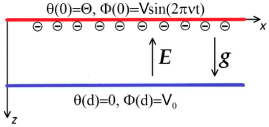
Figure 1.
Problem geometry and coordinate system.
The density of a liquid dielectric linearly depends on temperature:
We use dimensionless variables by choosing the following scales: time—d2/, length—d, velocity—/d, pressure—/, temperature— electric potential [Φ] = V0, and charge density [q] = ( is the electric constant), and write the system of electro-thermo-convection equations for an incompressible liquid [17]:
where v is the liquid velocity, and p is the pressure.
The buoyancy force and the Coulomb force act on some volume of liquid (3). The charge balance Equation (4) contains the convective transport and the charge mobility in the electric field. In our case (Equations (3)–(6)) of unipolar injection, only one type of carrier (negative charge) is generated on the cathode due to redox electrochemical reactions. The dielectric liquid has no residual conductivity and, therefore, no positive carriers. We consider the case of the autonomous injection from the cathode when the injected charge value does not depend on the electric field [3].
For the no-slip, perfectly heat-conducting electrodes, we write the boundary conditions:
The system of Equation (3) contains the following dimensionless parameters: the Prandtl number, , the electric Rayleigh number, T = 𝜀/𝐾, the charge mobility parameter, , the Rayleigh number,. Note that when the layer is heated from above, the temperature difference , and therefore, the Rayleigh numbers are negative.
The electric Rayleigh number T is a measure of the ratio of Coulomb force and viscous dissipative forces; it is analogue of the Rayleigh number. is the ratio of “hydrodynamic” mobility to ionic mobility [33]; it can vary over a wide range: 4 < M < 120 [3].
The parameter = / in boundary conditions (7) determines the injection strength ( is the charge injected into the liquid from the cathode). The dimensionless injection is the ratio of the injected charge per unit area to the surface charge that it would be present on the electrodes due to the applied external field /d [33].
3. Linear Stability Analysis
In the mechanical equilibrium state (v = 0), the temperature, the charge, and potential distributions can be written in the following form:
where is an auxiliary parameter associated with the charge at the cathode by the ratio
For each , the is first determined, and then distributions and are obtained. For example, the injection strength = 0.224 corresponds to the value 0.25, and the injection strength = 1.0 corresponds to the value 1.58.
Under heating of the layer from above, oscillatory instability appears as a result of the interplaying of two forces (the buoyancy force appearing due to the difference in the densities of heated liquid volumes and the Coulomb force acting on the negative charges injected from the cathode).
To analyze the stability of the quiescent liquid (so-called conductive state, ) relative to small disturbances, we consider perturbed fields of vertical velocity, electric potential, volume charge, and temperature as follows:
and will consider the solution in the form of 2D disturbances [25].
where w(z), q(z), Φ(z), and ϑ(z) are the amplitudes of disturbances, k is the wave number characterizing their spatial period, and λ is the growth rate. Substituting perturbations (9).
Here, the prime indicates differentiation with respect to the transverse coordinate z.
We carry out the linear stability analysis of the basic state (8) by solving the spectral-amplitude problem (10). The numerical procedure is based on the shooting method with the orthogonalization scheme for integration [33]. We have tested the results of linear stability in the absence of heating by comparing our data with the results of [34]. In both cases, for the injection parameter 0.1, the critical electric number is 24,147.
Figure 2 shows the marginal instability curves for the monotonic and oscillatory electro-thermo-convection for different values of charge mobility M and two values of the Rayleigh numbers: Ra = −2500, −1000. The monotonous instability regions are located above the black curves. The oscillatory instability regions are located between dashed blue and solid black lines.
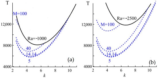
Figure 2.
The boundaries of the marginal instability for monotonic (solid black lines) and oscillatory (dashed blue lines) disturbances at different mobility parameters M and Rayleigh number values. (a) Ra = −1000; (b) Ra = −2500; = 0.224, Pr = 10.
The marginal instability curves for monotonic disturbances (k) and, therefore, the critical electric Rayleigh number and the critical wave number for monotonic instability (λ = 0) do not depend on the charge mobility M. This behavior can be explained by the properties of the system (6). In the case of λ = 0, the simultaneous substitution of parameters using the following scaling,
does not change Equation (10). Hence, the critical parameters , for monotonic disturbances also remain unchanged.
On the other hand, the intensity of heating strongly affects these critical values , grow with increasing of the Rayleigh number (). At the same time, the range of wave numbers in which oscillatory perturbations grow is expanded.
An increase in parameter M at fixed Ra shifts threshold for the oscillatory instability up and narrows the range of wave numbers , where oscillatory perturbations grow: the intersection point of the marginal curves for monotonic and oscillatory perturbations is shifted to the region of smaller k (Figure 2, dashed blue lines).
Figure 3 illustrates the dependences of the critical electric Rayleigh number , the frequency of marginal oscillations and the critical wavenumber on charge mobility M. The thresholds of the oscillatory instability (solid blue lines in Figure 3a) increases with M, while marginal oscillation frequency (blue dashed lines in Figure 3a) and the critical wavenumber corresponding to oscillatory perturbations (solid blue lines in Figure 3b) decreases. When the charge mobility is greater than some critical value , the global minimum of the neutral curve (for example, Figure 2) corresponds to the monotonic disturbances (black lines in Figure 3). For = 1.0 and Ra = –2500, the value of is 35.
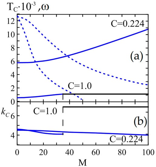
Figure 3.
Effect of mobility M of charge carriers on the critical values of (a) electric Rayleigh number and frequency of oscillations, (b) wavenumber for monotonous (black lines) and oscillatory (blue lines) disturbances. = 0.224, = 1.0, Ra = –2500, Pr = 10.
The dependences of the critical electric Rayleigh number on the Rayleigh number for different levels of charge injection (parameter ) are shown in Figure 4. As the injection level increases, the thresholds for monotonic and oscillatory convection decrease. It happens because a stronger injection imparts a larger charge to the liquid volume, and the Coulomb forces acting on the liquid are greater. Accordingly, the movement of a charged but a colder (and, hence, heavier) element of the liquid to the cathode (up) becomes easier. It should be noted that the value of the Rayleigh number for which oscillatory perturbations become dangerous depends on parameter . Calculations show that ≈ −177 for = 0.224 and ≈ −500 for = 1.0.
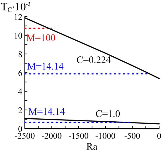
Figure 4.
Dependences of thresholds of monotonic (solid lines) and oscillatory (dashed lines) instabilities on the Rayleigh number for different values of parameter = 0.224, = 1.0, Pr = 10. Red line corresponds to M=100; blue lines correspond to M=14.14.
4. Nonlinear Electro-Thermo-Convection: Method of Solution and Characteristics of Wave Regimes
Numerical simulation of 2D wave regimes of electro-thermo-convection is carried out with the help of the two-field method: in the Navier–Stokes equation, instead of pressure p and velocity v, stream function ψ and the vorticity φ are used [10,25].
The system of Equation (3) is written in the following form:
We impose periodic boundary conditions along the x-axis with period l for all functions describing the electro-thermo-convection:
where
The system (12)–(16) with boundary conditions (17), (18) is solved by means of the finite-difference method. The balance equation for vorticity (12) is solved on the basis of an explicit scheme. The switching of calculations from the algorithm with central differences to the algorithm with “upwind” differences and back is performed depending on the stability criterion [10]. For the balance equations for heat and charge (16), (13), we apply an explicit scheme. Both the Poisson equations for the stream function (14) and the electric potential (15) are solved using the iterative method of successive over-relaxation at each time step. We use the grid with steps . The further mesh refinement did not show any sensible improvement in the calculation results.
The electro-thermo-convective flows are classified based on the behavior of the maximal , the minimal and local values of the stream function in a computational domain: ,
where local value is the stream function at a fixed point (x0 = l/4, z0 = ½).
We also use the Fourier spectrum A ( of the temporal oscillations and the phase velocity of the traveling wave defined as the derivative of the horizontal coordinate of the stream function maximum:
Simulations show that the vertical coordinate of this maximum for the electro-thermo-convective flows is = 1/2.
The spatiotemporal field distributions of stream function as well as the expansion of this field into the Fourier series in spatial harmonics, make it possible to characterize in detail the features of various flows of the liquid dielectric. We confine our analysis to the expansion of the stream function in the lateral direction in the cross-section at the height (z = 1/2):
For describing the structures formed in the liquid in our case, it is sufficient to use the information on the first , the second and the third harmonics of the stream function expansion.
All subsequent calculations are performed for the following values of parameters typical for dielectric liquids: Ra = −2500, Pr = 10, M = 14.14, and = 0.224; 1.0 [10,11,17,21]. An example of liquids that are similar in properties to this set of parameters can be ethanol with chlorine ions [3] or cyclohexane with the addition of triisoamylammonium perchlorate salt and tetramethylphenylenediamine filling a capacitor with stainless steel electrodes [8]. In [8], the electrode gaps are 0.1 mm–1.5 mm, and electric field strength varies from 0 to 100 kV/cm to study unipolar homogeneous injection. For further estimates, we will use the distance between the electrodes, 1.5 mm, and the voltage between the electrodes, 405 V (E = 2.7 kV/cm).
In order to verify the numerical method, we compare the results of the linear theory with the results of calculations in the fully nonlinear problem. For , the critical value for the oscillatory instability , which is obtained in nonlinear calculations, differs from the results of the linear theory by less than 1.5%; for example, Ra = −2500, M = 14.14: = 6905, and = 6805. The difference in frequencies at the threshold of electro-thermo-convection is approximately the same (2%;
5. Nonlinear Electro-Thermo-Convection: Results and Discussion
5.1. DC Electric Field
Here, we discuss the bifurcation and spatiotemporal properties of the electro-thermo-convective states of a dielectric liquid in the steady electric field, α = 0. The bifurcation map of the solutions for Ra = −2500 in the case of moderate injection = 1.0 is shown in Figure 5.
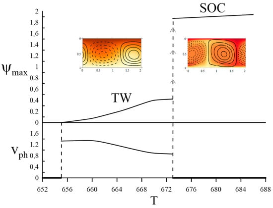
Figure 5.
The bifurcation map of the electro-thermo-convective solutions: the maximum value of the stream function and the phase velocity versus the electric parameter T; = 1.0, l = 1.44. Left insert: snapshots of the stream function and temperature for the traveling wave; right inset: snapshots of the stream function and temperature for the steady overturning convection.
This map contains the dependences of the maximal value of the stream function and the phase velocity on the electric Rayleigh number T. In the region liquid is quiescent ( = 0), and the distributions of charge density q0(z) and electric field depend only on transverse coordinate z (conductive state). Electro-thermo-convection arises at the electric parameter as a result of forward Hopf bifurcation (Figure 5). In the region T > , the oscillatory disturbances growth, and the traveling wave solution appears as a result of the transient process (Figure 6, t > 80). The traveling wave (TW, Figure 5) exists in the range of the electric Rayleigh number .
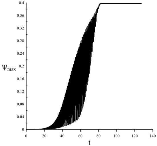
Figure 6.
Time evolution of maximal value of the stream function = 1.0, l = 1.44.
The two electro-thermo-convective rolls rotating in opposite directions form one spatial period l of the TW solution (Figure 5, insert). In our consideration, all fields characterizing this flow (the stream function, the temperature, the charge density, and the electric potential) are shifted to the left with a constant phase velocity, while the maximal value of the stream function remains constant at fixed T. Despite the lateral motion of the traveling wave, the total fluid flow along the horizontal axis is zero. This is easy to prove using boundary conditions for the stream function:
For cyclohexane with salt additives [8] (), we obtain the electric Rayleigh number T = 670, which corresponds to the interval in which numerical simulation predicts the existence of a traveling wave.
With further increase in the electric Rayleigh number (T > 671, Figure 5), the intensity of electro-thermo-convection sharply grows, and the regime of stationary overturning convection is formed (Figure 5, the transition is marked with an up arrow SOC). This regime is characterized by mirror symmetry between rolls that rotate in opposite directions (Figure 5, right insert). The maximal value of the stream function = 2 is much greater than in the traveling wave mode. The phase velocity of the traveling wave decreases monotonically with increasing electric Rayleigh number.
With a decrease in the parameter , the range of stable traveling waves shifts towards large values of the electric Rayleigh number. For = 0.224, TW exists in the interval 6818 < T < 7037.
5.2. AC Electric Field
If we change the electric potential on the cathode with the frequency and the amplitude of α, new oscillatory solutions can be generated.
If the modulation amplitude does not exceed a certain critical value in general, the oscillations of the stream function have two different frequencies, and these dynamics correspond to modulated traveling waves (MTW). The evolution of the flow versus time and the Fourier spectrum of the are shown in Figure 7 for = 0.224, T = 6950. The Fourier spectrum (Figure 7b) contains a few frequencies which are the combination of the fundamental frequency of the traveling wave in the unmodulated case and the modulation frequency . The largest peak corresponds to , and the height of the peaks at in the spectrum is smaller. If the external frequency coincides with the fundamental oscillation frequency , the spectrum looks simpler (Figure 7d). It contains only multiples of frequencies; we have periodic TW.
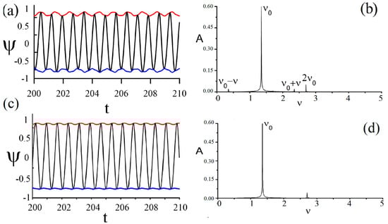
Figure 7.
(a,c) The oscillations of the stream function (black lines) and its envelopes (red lines for , blue lines for ) and (b,d) their Fourier spectrum at ν = 1, α = 0.03 (a,b) and ν = 1.35, α = 0.01 (c,d). Parameters are Ra = −2500, Pr = 10, M = 14.14, = 0.224, T = 6950, l = 2.
The modulation of the field causes a change in the amplitude of the spatial harmonics (Figure 8). The behavior of harmonics is different for different frequency ratios . In the most common case, the characteristic frequencies and of the MTW solution is not rationally related to each other. The oscillations of the first harmonic amplitude (red line Figure 8a) is an example of such a quasiperiodic TW with 0.74074. Thus, the trajectory of (Figure 8b) is not closed, and orbits fill the area between = 0.83 and = 0.77. In Figure 8d–f, we show the trajectories for periodic TWs with Q = 1 and 2, respectively. Here, the orbits of are closed after one and two periods of , respectively. The contribution of the second harmonic = 0.098 does not exceed 13% of the contribution from the first harmonic. The contribution of the third harmonic is small, = 0.04. The behavior of the third harmonic (blue line in Figure 8) corresponds to a standing wave. The contribution of higher harmonics is even smaller:
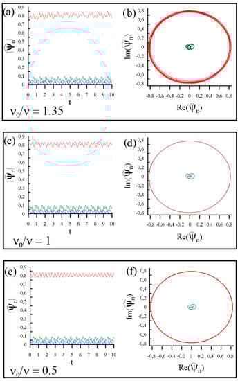
Figure 8.
(a,c,e) Evolution of the lateral Fourier modes of in the expansion (12) of the stream function : and (b,d,f) their trajectories in the plane spanned by the real and imaginary parts of .
If the modulation amplitude α exceeds a certain critical value , the MTW loses stability, and a more intensive oscillating solution is formed in a liquid dielectric (Figure 9). In this modulated electroconvective (MEC) regime, the flow amplitude varies in some intervals ( synchronously with the potential difference around the unmodulated SOC solution.
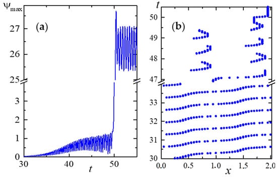
Figure 9.
The emergence of the modulated electroconvection regime (MEC) from the modulated traveling wave. (a) The time evolution of the maximal value of the stream function, (b) behavior of the x-coordinate of the stream function maximum on the world line plot; Pr = 10, M = 14.14, = 0.224, Ra = −2500, T = 6950, ν = 2, α = 0.05, l = 2.
Let us consider the transient process from the MTW to the MEC solution, which is illustrated in for and . The change in the spatial position (x-coordinate) of is depicted on the world line plot (Figure 9b, 30 < t < 52, blue circles). The lateral motion of convective rolls along the layer takes place. It can be seen from Figure 9b that the traveling wave propagates from left to right, and it is phase-modulated: the phase velocity of the wave is equal to the inverse slope to the t(x) line.
In the time interval 47.5 < t < 50, the position of the maximum of the stream function oscillates in the interval of coordinates 0.5 < x < 0.8 and 1.5 < x < 1.8, leaving “horseshoe” traces on the world line plot. The left boundaries of these intervals (x = 0.5 and x = 1.5) correspond to the positions of extrema of the first spatial harmonic, and oscillations themselves are associated with changes in the second harmonic amplitude. After the external period, switching occurs: the position of the maximum is shifted by half-length of the cell (±/2). If t > 50, the x-coordinate of does not change. There is no movement of convective structures in the horizontal direction. The transient process is finished, and the modulated electroconvective flow is formed.
The dependence on the critical value of the amplitude () on frequency is the boundary between the modulated traveling wave (MTW) and the modulated electroconvection (MEC). Such dependence (𝜈) at = 0.224, T = 6950 is shown in Figure 10a. Below this curve, the MTW regime is stable; above this boundary, modulated electroconvection (MEC) is stable. The dependence is not monotonic; it has local minima and maxima. The frequencies of the minima have specific values which correspond to the ratio /𝜈 = 𝑛/2, 𝑛 = 1, 2, 4. This confirms the presence of parametric resonance in the system. The absolute minimum at the boundary of parametric instability of the MTW is clearly manifested (the first resonance tongue). It corresponds to the external frequency that is twice the fundamental one (𝜈 = 2, 𝑛 = 1). Due to the presence of dissipation in the convective system, the remaining minima (resonance tongues) are not so sharp and are located much higher in amplitude.
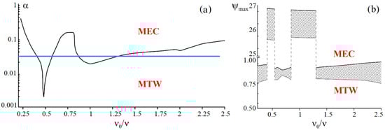
Figure 10.
(a) The boundary between modulated traveling wave and modulated electroconvection; (b) Range of amplitude variation as a function of frequency at . Pr = 10, M = 14.14, C = 0.224, Ra = −2500, T = 6950, l = 2.
However, the dependence corresponding to the parametric excitation of modulated electroconvection is slightly different from the classical Floquet theory of parametric instability [35]: 𝜈 = 2𝜈0/𝑛, 𝑛 = 1, 2, 3… There is no minimum of a curve with a frequency ratio of 𝜈0/𝜈 = 3/2. This difference is not surprising because the considered system is explicitly nonlinear.
Interval of amplitude variation as a function of frequency is shown in Figure 10b at . The lower shaded regions correspond to the modulated traveling wave. One can see that the ratio of frequencies 𝜈0/𝜈 = 0.75 between the first two resonant tongues is the least favorable for parametric excitation of the modulated electroconvection: range of amplitude variation here is minimum (Figure 10b, 𝜈0/𝜈 = 0.75). With an increase in the period of external modulation (growth of the ratio 𝜈0/𝜈), the interval of amplitude variation of the solutions grows.
The upper regions in Figure 10 correspond to the solutions located inside the resonant tongues and characterize modulated electroconvection (MEC). As follows from the theory of parametric resonance [36], the conditions for energy transfer from an external source to the system are more favorable in the first resonant tongue 0.40 < 𝜈0/𝜈 < 0.58, so the interval of change in the amplitude of the response is greater there than in the second resonant tongue 0.87 < 𝜈0/𝜈 < 1.3.
Using an alternating electric field, it is possible to control the intensity of convection and, consequently, heat transfer. Changing the excitation frequency switches the low-intensity flow to a more intense one.
6. Conclusions
Electro-thermo-convection of a dielectric liquid subject to autonomous unipolar injection from the cathode and heating from above have been investigated in the external DC and AC electric fields. The linear stability analysis was carried out in the case of a DC electric field. The critical wave and Rayleigh numbers, as well as frequencies of marginal oscillations, were determined. The spatiotemporal behavior and the bifurcation properties of oscillating electro-thermo-convection have been analyzed with the help of finite difference numerical simulations. Traveling waves and the regime of stationary overturning convection are found at the moderate .
Parametric excitation of instability takes place in the case of an AC electric field. The low-intensity modulated traveling waves (MTW) and the high-intensity modulated electroconvection (MEC) were found as stable solutions. An analysis of the spatial harmonics made it possible to elucidate the properties of modulated traveling waves at various frequencies of the external field. The characteristics of oscillatory instability in a DC electric field provide important predictive information for the analysis of electro-thermo-convection in an AC field.
Author Contributions
Conceptualization, O.N. and B.S.; formal analysis, O.N. and B.S.; funding acquisition, B.S.; investigation, O.N. and B.S.; project administration, B.S.; software, O.N.; Validation, O.N. and B.S.; visualization, O.N. and B.S.; writing—original draft, O.N. and B.S.; writing—review and editing, O.N. and B.S. All authors have read and agreed to the published version of the manuscript.
Funding
This research was funded by Russian Science Foundation, No. 23-21-00344, https://rscf.ru/en/project/23-21-00344/.
Data Availability Statement
The datasets generated during and/or analyzed during the current study are available from the corresponding author upon reasonable request.
Conflicts of Interest
The authors declare no conflict of interest. The funders had no role in the design of the study; in the collection, analyses, or interpretation of data; in the writing of the manuscript; or in the decision to publish the results.
References
- Melcher, J.R. Continuum Electromechanics, 1st ed.; MIT Press: Boston, MA, USA, 1981. [Google Scholar]
- Gross, M.J.; Porter, J.E. Electrically induced convection in dielectric liquids. Nature 1966, 212, 1343–1345. [Google Scholar] [CrossRef]
- Lacroix, J.C.; Atten, P.; Hopfinger, E.J. Electroconvection in a dielectric liquid layer subjected to unipolar injection. J. Fluid Mech. 1975, 69, 539–563. [Google Scholar] [CrossRef]
- Ostroumov, G.A. Interaction of Electric and Electrohydrodynamic Fields; Nauka: Moscow, Russia, 1979. (In Russian) [Google Scholar]
- Castellanos, A.; Velarde, M.G. Electrohydrodynamic stability in the presence of a thermal gradient. Phys. Fluids 1981, 24, 1784–1786. [Google Scholar] [CrossRef]
- Mutabazi, I.; Yoshikawa, H.N.; Fogaing, M.T.; Travnikov, V.; Crumeyrolle, O.; Futterer, B.; Egbers, C. Thermo-electro-hydrodynamic convection under microgravity: A review. Fluid Dyn. Res. 2016, 48, 061413. [Google Scholar] [CrossRef]
- Pontiga, F.; Castellanos, A. Physical mechanisms of instability in a liquid layer subjected to an electric field and a thermal gradient. Phys. Fluids 1994, 6, 1684–1701. [Google Scholar] [CrossRef]
- Denat, A.; Gosse, B.; Gosse, J.P. Ion injections in hydrocarbons. J. Electrost. 1979, 7, 205–225. [Google Scholar] [CrossRef]
- Tobazeon, R. Electrohydrodynamic instabilities and electroconvection in the transient and A.C. regime of unipolar injection in insulating liquids: A review. J. Electrost. 1984, 15, 359–384. [Google Scholar] [CrossRef]
- Vereshchaga, A.N.; Tarunin, E.L. Supercritical modes of unipolar convection in a closed cavity. In Numerical and Experimental Simulation of Hydrodynamic Phenomena under Weightlessness; Briskman, V.A., Ed.; Ural Branch of the Academy of Sciences of the Soviet Union: Ekaterinburg, Russia, 1988; pp. 92–99. (In Russian) [Google Scholar]
- Mordvinov, A.N.; Smorodin, B.L. Electroconvection under injection from cathode and heating from above. J. Exp. Theor. Phys. 2012, 114, 870–877. [Google Scholar] [CrossRef]
- Smorodin, B.L. Wave regimes of electroconvection under cathode injection and heating from above. J. Exp. Theor. Phys. 2022, 134, 112–122. [Google Scholar] [CrossRef]
- Malrison, B.; Atten, P. Chaotic behaviour of instability due to unipolar injection in a dielectric liquid. Phys. Rev. Lett. 1982, 49, 723–726. [Google Scholar] [CrossRef]
- Polyanskiǐ, V.A.; Pankrat’eva, I.L. Generation of strong electric fields by fluid flows in narrow channels. Dokl. Phys. 2005, 50, 397–400. [Google Scholar] [CrossRef]
- Polyansky, V.A.; Pankrat’eva, I.L. Electric current oscillations in low-conducting liquids. J. Electrost. 1999, 48, 27–41. [Google Scholar] [CrossRef]
- Zhang, Y.; Chen, D.; Liu, A.; Luo, K.; Wu, J.; Yi, H.-L.; Yi, H.-L. Full bifurcation scenarios and pattern formation of laminar electroconvection in a cavity. Phys. Fluids 2022, 34, 103612. [Google Scholar] [CrossRef]
- Traore, P.; Perez, A.T.; Koulova, D.; Romat, H.J. Numerical modelling of finite-amplitude electro-thermo-convection in a dielectric liquid layer subjected to both unipolar injection and temperature gradient. J. Fluid Mech. 2010, 658, 279–293. [Google Scholar] [CrossRef]
- Smorodin, B.L.; Taraut, A.V. Parametric convection of a low-conducting liquid in an alternating electric field. Fluid Dyn. 2010, 45, 1–9. [Google Scholar] [CrossRef]
- Su, Z.-G.; Li, T.-F.; Su, W.-T.; Yi, H.-L. Numerical simulation of electrothermal convection in dielectric liquids enclosed within rectangular cavities. Fluid Dyn. 2021, 56, 922–935. [Google Scholar] [CrossRef]
- Li, T.F.; Luo, K.; Yi, H.L. Suppression of Rayleigh-Bénard secondary instability in dielectric fluids by unipolar charge injection. Phys. Fluids 2019, 31, 064106. [Google Scholar] [CrossRef]
- Selvakumar, R.D.; Wu, J.; Huang, J.; Traoré, P. Electro-thermo-convection in a differentially heated square cavity under arbitrary unipolar injection of ions. Int. J. Heat Fluid Flow 2021, 89, 108787. [Google Scholar] [CrossRef]
- Il’in, V.A.; Aleksandrova, V.N. Wave Regimes of Electroconvection of a Low Conducting Liquid under Unipolar Injection of a Charge in a Steady Electric Field. J. Exp. Theor. Phys. 2020, 130, 293. [Google Scholar] [CrossRef]
- Nekrasov, O.O.; Smorodin, B.L. Effect of charge modulation on the electroconvective flow of a low conducting liquid. Math. Model. Nat. Phenom. 2021, 16, 35. [Google Scholar] [CrossRef]
- Kapitza, P.L. Dynamic stability of a pendulum with an oscillating point of suspension. J. Exp. Theor. Phys. 1951, 21, 588–597. [Google Scholar]
- Gershuni, G.Z.; Zhukhovitsky, E.M. Convective Stability of Incompressible Fluids; Keter: Jerusalem, Israel, 1976. [Google Scholar]
- Nepomnyashchy, A.; Symanovskii, I. Generation of nonlinear Marangoni waves in a two-layer film by heating modulation. J. Fluid Mech. 2015, 771, 159–192. [Google Scholar] [CrossRef]
- Smorodin, B.L.; Lücke, M. Convection in binary fluid mixtures with modulated heating. Phys. Rev. E 2009, 79, 026315. [Google Scholar] [CrossRef] [PubMed]
- Smorodin, B.L.; Kartavykh, N.N. Periodic and chaotic oscillations in a low conducting liquid in an alternating electric field. Microgravity Sci. Technol. 2020, 32, 423–434. [Google Scholar] [CrossRef]
- Smorodin, B.L.; Taraut, A.V. Dynamics of electroconvective wave flows in a modulated electric field. J. Exp. Theor. Phys. 2014, 118, 158–165. [Google Scholar] [CrossRef]
- Zhou, C.-T.; Yao, Z.-Z.; Chen, D.-L.; Luo, K.; Wu, J.; Yi, H.-L. Numerical prediction of transient electrohydrodynamic instabilities under an alternating current electric field and unipolar injection. Heliyon 2023, 9, e12812. [Google Scholar] [CrossRef]
- Atten, P.; McCluskey, F.M.J.; Perez, A.T. Electroconvection and its effect on heat transfer. IEEE Trans. Electr. Insul. 1988, 23, 659–667. [Google Scholar] [CrossRef]
- McCluskey, F.M.J.; Atten, P.; Perez, A.T. Heat transfer enhancement by electroconvection resulting from an injected space charge between parallel plates. Int. J. Heat Mass Tran. 1991, 34, 2237–2250. [Google Scholar] [CrossRef]
- Ascher, U.M.; Mattheij, R.M.M.; Russell, R.D. Numerical Solution of Boundary Value Problems for Ordinary Differential Equations; Prentice Hall Series in Computational Mathematics; Prentice-Hall: Englewood Cliffs, NJ, USA, 1988. [Google Scholar]
- Castellanos, A.; Atten, P. Numerical modeling of finite amplitude convection of liquids subjected to unipolar injection. IEEE Trans. Ind. Appl. 1987, IA-23, 825–830. [Google Scholar] [CrossRef]
- Coddington, E.A.; Levinson, N. Theory of Ordinary Differential Equations; McGraw-Hill: New York, NY, USA, 1955. [Google Scholar]
- Rabinovich, M.I.; Trubetskov, D.I. Introduction to the Theory of Oscillations and Waves; Kluwer: Dordrecht, The Netherlands, 1989. [Google Scholar]


Disclaimer/Publisher’s Note: The statements, opinions and data contained in all publications are solely those of the individual author(s) and contributor(s) and not of MDPI and/or the editor(s). MDPI and/or the editor(s) disclaim responsibility for any injury to people or property resulting from any ideas, methods, instructions or products referred to in the content. |
© 2023 by the authors. Licensee MDPI, Basel, Switzerland. This article is an open access article distributed under the terms and conditions of the Creative Commons Attribution (CC BY) license (https://creativecommons.org/licenses/by/4.0/).