Association Testing of a Group of Genetic Markers Based on Next-Generation Sequencing Data and Continuous Response Using a Linear Model Framework

Abstract

Association testing has been widely used to study the relationship between phenotypes and genetic variants. Most testing methods are based on genotypes. To avoid genotype calling and directly test on next-generation sequencing (NGS) data, sequencing data-based methods have been proposed and shown advantages over genotype-based testing methods in scenarios where genotype calling is inaccurate. Most sequencing data-based testing methods are based on a single genetic marker. The objective of this paper is to extend the methods to allow testing for the association of a continuous response variable with a group of common variants or a group of rare variants without genotype calling. Our proposed methods are derived based on a standard linear model framework. We derive the joint significant test (JS) for a group of common genetic variables and the variable collapse test (VC) for a group of rare genetic variables. We have conducted extensive simulation studies to evaluate the performance of different estimators. According to our results, we found (1) all methods, including our proposed NGS data-based methods and genotype-based methods, can control the Type I error rate probability well; (2) our proposed NGS data-based methods can achieve better performance in terms of statistical power compared with their corresponding genotype-based methods in the literature; (3) when sequencing depth increases, the performance of all methods increases, and the difference between the performance of NGS data-based methods and corresponding genotype-based methods decreases. In conclusion, we have proposed NGS data-based methods that allow testing for the significance of a group of variants using a linear model framework and have shown the advantage of our NGS data-based methods over genotype-based methods in the literature.

1. Introduction

With recent advances in sequencing technology, next-generation sequencing (NGS) has become increasingly popular in genetic association studies. The new technologies have lower costs and higher sequencing throughput compared with traditional technologies, such as Sanger sequencing [1]. Massive sequencing data have been generated for genetic studies from NGS platforms, such as Solexa and Solid [2,3].

Next-generation sequencing (NGS) data in the format of raw sequencing reads are collected from NGS platforms [4,5,6]. There are no genotype data provided by these platforms. To obtain genotype data, multiple processing procedures, including quality control, sequence alignment, genetic variant calling and genotype calling (GC), have to be conducted [5,7,8]. Genotype calling is the process of determining the genotype for each individual and is typically only performed for positions in which a SNP or a ’variant’ has already been called [9]. Genotype calls refer to the estimated genotypes obtained by genotype calling [9]. Bioinformatics pipelines have been developed to obtain genotype calls based on NGS data [10,11,12]. Based on these obtained genotypes, association testing is conducted to study how genotypes and other variables (environmental factors, socioeconomic factors, etc.) are associated with phenotypes [9,13,14].

Regression models have been used to develop association testing approaches. Phenotypes are responses. Explanatory variables include genotypes and other variables, such as batch effects, environmental variables, socioeconomic status and behavioral variables. To model a continuous phenotype, researchers adopt linear models or linear mixed models depending on whether individual observations are independent or not [15,16]. Random effects can be used to control the relatedness of individuals. For example, when individuals contain multiple persons from the same family, which can be detected by checking whether different persons have the same family identifier, they are related individuals instead of independent individuals.

To test for association between genetic variables and the phenotype, different strategies are recommended depending on whether genetic variables are common variants or rare variants. A genetic marker can be classified as a common variant or a rare variant depending on whether its minor allele frequency (MAF) is higher or lower than a threshold value c, which is between 0.01 and 0.05 [17,18]. For common markers, association testing can be based on an individual marker assuming a genetic dominant or recessive or additive model, and genome-wide association studies (GWAS) are used to repeat the individual-marker test for all common markers genome-wide [9,19]. Other testing methods for common markers include testing for a group of common markers, which can be F tests and Chi-square tests of the joint significance of explanatory variables in linear models [20,21]. Group testing can be gene-based, pathway-based or range-based. Gene-based group testing treats all genetic markers within the same gene as a group. Pathway-based group testing treats all genetic markers within the same pathway as a group. Range-based testing divides chromosomes into different genomic regions. For example, range-based testing can divide chromosomes into intervals of a fixed length, such as 1 Mb, and then group testing treats all genetic markers within the same interval (genomic region) as a group. All genetic markers in the same group are tested simultaneously using a group test. Genome-wide group testing refers to repeating the individual group testing for all groups genome-wide.

Rare variants are characteristics of low variations in genotypes since their minor allele frequencies (MAF) are less than a pre-specified threshold value, typically 0.05. Thus, there may not be enough statistical power for the association testing of a single rare variant [17,22]. Testing of rare variants is usually performed on a group of rare markers instead of a single marker. The group of rare variants can be within a genomic region (range-based), within a gene (gene-based) or within a pathway (pathway-based) [22,23].

A range of rare-variant testing methods has been proposed, and different methods have been compared [17,22]. Among all the rare-variant tests, two big categories of rare-variant testing methods are widely used. The first category is by variable collapsing, which first combines multiple genetic variables into one variable or calculates an index based on multiple genetic variables. It then tests the association between phenotype and the merged variable or the index [24,25]. Within the first category of methods, i.e., variable collapse (VC) methods, the burden test is a widely-used method, which first calculates the sum of rare alleles and then conducts regression of the phenotype on the number of rare alleles and other covariates [23,25]. The second category is the variants of Sequence Kernel Association testing (SKAT) methods. The second category of methods includes SKAT, MK-SKAT, BESKAT and SKAT-O [17,24,26,27].

The burden test and the SKAT test are, respectively, representative methods of the two categories of rare-variant testing methods [25,27]. They have been widely used in association studies of a group of rare variants with phenotypes. Both tests are genotype-based tests in that they first conduct genotype calling to obtain or estimate genotypes and then conduct association testing based on phenotypes and the estimated genotypes.

However, there are uncertainties and errors in obtaining genotypes by genotype calling. Multiple factors influence genotyping accuracy, such as mapping accuracy, sequencing errors and sequencing depth. There may only be a few sequencing reads at some specific locations, i.e., low sequencing depth, which makes genotype calling imprecise. Uncertainty in genotype calling may influence downstream genotype-based association studies [28,29]. To improve genetic studies of genomic locations, alternative testing approaches avoiding genotype calling have been proposed. Directly modeling next-generation sequencing (NGS) data instead of genotypes considers uncertainty and errors in genotype calling and improves statistical performances in association testing [30,31].

Recent technological advances and real situations motivate the development of NGS data-based methods. One reason is the decreasing costs and increasing throughputs in recent sequencing technologies. Massive sequencing data have been generated and are available to researchers, whereas there are no direct genotype calls provided by these sequencing platforms [2,32]. The second reason is that many large studies on the genotype-phenotype relationship have their samples or individuals sequenced at a low depth with the purpose of increasing sample sizes given budget constraints. Genotype calling from low-sequencing data has uncertainty [33]. Considering uncertainty in genotype calls may improve association testing performance [31]. However, commonly-used association testing approaches ignore the uncertainty and use only one single value to represent the genotype [14,34,35]. The single genotype value used in testing is the best-guess genotype or the expected genotype, i.e., dosage, in association testing [36,37]. Ignoring genotype calling uncertainty influences association testing performance. The third reason is that there may be different sequencing depths. For example, in case-control studies, sequencing data in the case group and control group may have different sequencing depths. This difference in sequencing depth may influence the case-control study results [38]. Another example is that researchers may have sequencing data with different depths. Researchers have to choose whether to use a smaller data set with similar sequencing depths or a larger data set with heterogeneous sequencing depths. Researchers have to ignore the bias due to heterogeneous depth or correct for sequencing depth, such as the inclusion of it as an additional covariate [31,39]. NGS data-based association testing methods can avoid time-consuming and likely imprecise genotype calling and directly model NGS data. The fourth reason is from the perspective of information theory. Genotypes are obtained from the proceeding NGS data that results in a loss of information. To maximize the information that is used, association testing based on sequencing data is preferred and expected to have better or at least the same performance as genotype-based testing methods.

Researchers have proposed association testing methods based on sequencing data without genotype calling [30,31,40]. The methods can achieve better performance under the scenario of low sequencing depth, heterogeneous sequencing depths and imprecise genotype calls [30,31,40]. However, most of these methods are designed for the testing of a single marker. Testing for a group of genetic markers is also crucial, and there have been a range of genotype-based group-testing methods for common variants (joint significance test) and rare variants (burden test and SKAT test) [24,27,41]. There are no sequencing data-based testing methods for a group of markers developed in the literature using the statistical framework of linear models. We fill the literature gap by developing sequencing data-based testing methods for the association of a continuous phenotype with a group of genetic markers based on independent individuals using a standard linear model framework. We propose the joint significance test (JS) for a group of common variants and the variable collapse test (VC) for a group of rare variants. Their corresponding genotype-based testing methods are the F test and Chi-square test for a group of common variants and the burden test for a group of rare variants.

The rest of the article is organized as follows. Section 2 states the methodology, including the sequence-data joint significance test and variance collapse test. Section 3 shows the results of our simulation studies. Section 4 provides the discussion, and Section 5 draws conclusions.

2. Methodology

Suppose there are N individuals. For individual i, we have $(y_i,g_i,x_i)$, where $y_i$ is the phenotype, $g_i$ represents the genotypes and $x_i$ represents additional covariates, such as age, gender and environmental variables. Assume the genetic variants under consideration are bi-allelic so that the genotypes can only take values of 0, 1 and 2.

Suppose we consider a group of $d_g$ genetic variables in the test so that the genotypes of individual i are represented as a row vector $g_i=(g_{i1},g_{i2},\dots ,g_{i_{d_g}})$, where $g_{ij}$ is the genotype value at the j-th genetic variant for individual i. We allow our test to include $d_x$ additional covariates and let the row vector $x_i=(1,x_{i1},x_{i2},\dots ,x_{i{d}_x})$ represent the intercept and $d_x$ additional covariates, where $x_{ij}$ is the value of the j-th additional covariate for individual i.

For N individuals under consideration, we have the genotype matrix of size $N\times d_g$ as $g=(g_1,g_2,\dots ,g_N),$ response vector of length n as $y=(y_1,y_2,\dots ,y_N),$ and additional covariates matrix of size $N\times (d_x+1)$ as $x=(x_1,x_2,\dots ,x_N).$

2.1. Model Continuous Phenotype Using a Linear Model Framework

We model continuous phenotypes by a linear model (LM) framework. The derivation is a laborious extension of the work in Skotte et al., 2012 for NGS data-based association testing in an individual marker [30]. Skotte et al., 2012 represent the genotype of a single genetic marker as a variable taking only three possible values (i.e., 0, 1 and 2) and then derive the association test for this single marker based on NGS data without genotype calling [30]. In their article, they mentioned that an alternative way to test for this single marker with three genotype values is to use two dummy or binary variables that can only take two values, i.e., 0 and 1. Their derivations in association testing for a numerical genetic variable taking values of 0, 1 and 2 can be modified for the testing of two binary variables corresponding to this numerical variable, which is actually the representation of a categorical variable with levels 0, 1 and 2, instead of a numerical variable taking values 0, 1 and 2 [30,42].

Motivated by their statement, we further extend their work to allow for the testing of a group of multiple genetic variables, each taking three possible values, i.e., 0, 1 and 2. In this way, we extend Skotte et al., 2012’s testing method for a single genetic variable to our methods, which allows testing for a group of common variants. In addition, we also derive the variable collapse method (VC) for the testing of a group of rare variants based on NGS data. The derivation of the NGS data-based variable collapse method makes use of the chain rule in calculus.

We model a continuous phenotype using a linear model [43,44]. For individual i, his or her phenotype is modeled using the formula

$$y_i=\alpha x_i^T+\beta g_i^T+{ϵ}_i={\eta }_i+{ϵ}_i,{ϵ}_i\sim N(0,{\sigma }^2),$$

(1)

where the row vector $\alpha \in {\mathcal{R}}^{d_x+1}$ and the row vector $\beta \in {\mathcal{R}}^{d_g}$. Thus, $y_i\sim N({\eta }_i,{\sigma }^2)$, where ${\eta }_i=\alpha x_i^T+\beta g_i^T$, so that the distribution of the phenotype $y_i$ depends on the individual predictors ($x_i$ and $g_i$) as well as the parameters $(\alpha ,\beta ,\varphi )$, where $\varphi ={\sigma }^2$.

2.2. Uncertain Genotypes

Since the actual genotypes remain unobserved in NGS studies, we directly model the joint distribution of the phenotypes and the observed sequencing data. Because phenotypes are conditionally independent of the sequencing data given true genotypes, the density of the joint distribution can be factorized as

$$p_{\theta }(y_i,D_i|x_i)=\sum _{g\in \mathcal{G}}{f}_{\theta }\left(y_i\right|x_i,g)h(g,D_i),$$

(2)

where $\theta =(\alpha ,\beta ,\varphi )$, $y_i$, $D_i$ and $x_i$ are, respectively, the phenotype, sequencing reads and additional covariates for individual i. The term $\mathcal{G}$ is the genotype state space, including all possible genotype values g, which means that in Equation (2), the summation is over all possible values of g. Since there are $d_g$ genetic markers in testing, and each genetic marker takes possible values of 0, 1 or 2, then $\mathcal{G}={\{0,1,2\}}^{d_g}$. The term h in Equation (2) is the shorthand notation for the joint distribution of the genotype and the observed sequencing data, i.e., $h(g,D_i)=p\left(D_i\right|g)p\left(g\right|\widehat{f})$, where $\widehat{f}$ is the estimated allele frequency, as modeled in Skotte et al. (2012) [30]. The log-likelihood function for the model with genotype uncertainties (i.e., latent genotypes) thus becomes

$$l_{y,D}(\alpha ,\beta ,\varphi )=\sum _{i=1}^{N}log\left\{p_{\theta }(y_i,D_i|x_i)\right\}=\sum _{i=1}^{N}log\left\{\sum _{g\in \mathcal{G}}{f}_{\theta }\left(y_i\right|x_i,g)h(g,D_i)\right\}.$$

(3)

In this model, testing for genetic effects means testing with the null hypothesis $H_0$:$\beta =0$. Under this null hypothesis, the density f does not depend on the genotype, so it can be extracted out of the summation. Thus the log-likelihood function under this null hypothesis ($H_0$:$\beta =0$) can be simplified as follows:

$$\begin{array}{ccc}\hfill l_{y,D}(\alpha ,0,\varphi )& =& \sum _{i=1}^N(log\left(\sum _{g\in \mathcal{G}}{f}_{\theta }\left(y_i\right|x_i,g)h(g,D_i)\right))\hfill \\ & =& \sum _{i=1}^N\{\frac{y_i\left(\alpha x_i^T\right)-{\left(\alpha x_i^T\right)}^2/2}{\varphi }+c(y_i,\varphi )\}+\mathrm{constant}\mathrm{in}\mathrm{terms}\mathrm{of}\mathrm{parameters},\hfill \end{array}$$

where $c(y_i,\varphi )=-y_i^2/\left(2\varphi \right)-log\left(2\pi \varphi \right)/2$. We have provided full derivation details for this simplification in Appendix A.

Therefore, the constrained MLE under the null hypothesis ($H_0$:$\beta =0$) can be easily found from the linear regression of phenotype y on the additional covariates x only when no genotypes g show up in the formula ${\eta }_i=\alpha x_i^T+\beta g^T$ under $H_0$:$\beta =0$. This motivates us to develop our method using the score test because the score test considers the constrained MLE under $H_0$:$\beta =0$.

2.3. Joint Significance Test for a Group of Common Genetic Variants

We use a standard score test with our null hypothesis [45,46]. The score function is

$$\begin{array}{cc}\hfill s_{y,D}(\alpha ,\beta ,\varphi )& =\left[\begin{array}{c}\partial l_{y,D}(\alpha ,\beta ,\varphi )/\partial {\alpha }^T\\ \partial l_{y,D}(\alpha ,\beta ,\varphi )/\partial {\beta }^T\\ \partial l_{y,D}(\alpha ,\beta ,\varphi )/\partial \varphi \end{array}\right],\hfill \end{array}$$

(4)

where $\alpha$ is a row vector of length $d_x+1$, $\beta$ is a row vector of length $d_g$ and $\varphi$ is a scalar.

The observed information matrix is

$$\begin{array}{cc}\hfill o_{y,D}(\alpha ,\beta ,\varphi )& =-\left[\begin{array}{ccc}{\partial }^2{l}_{y,D}(\alpha ,\beta ,\varphi )/\partial {\alpha }^T\partial \alpha & {\partial }^2{l}_{y,D}(\alpha ,\beta ,\varphi )/\partial {\alpha }^T\partial \beta & {\partial }^2{l}_{y,D}(\alpha ,\beta ,\varphi )/\partial {\alpha }^T\partial \varphi \\ {\partial }^2{l}_{y,D}(\alpha ,\beta ,\varphi )/\partial {\beta }^T\partial \alpha & {\partial }^2{l}_{y,D}(\alpha ,\beta ,\varphi )/\partial {\beta }^T\partial \beta & {\partial }^2{l}_{y,D}(\alpha ,\beta ,\varphi )/\partial {\beta }^T\partial \varphi \\ {\partial }^2{l}_{y,D}(\alpha ,\beta ,\varphi )/\partial \varphi \partial \alpha & {\partial }^2{l}_{y,D}(\alpha ,\beta ,\varphi )/\partial \varphi \partial \beta & {\partial }^2{l}_{y,D}(\alpha ,\beta ,\varphi )/\partial \varphi \partial \varphi \end{array}\right].\hfill \end{array}$$

In the following, we denote the constrained maximum likelihood estimate of the parameters under the null hypothesis $H_0:\beta =0$ as $\tilde{\theta }=(\tilde{\alpha },0,\tilde{\varphi })$. The score statistic is

$$R(y,D)={\left[s_{y,D}(\tilde{\alpha },0,\tilde{\varphi })\right]}^T{\left[o_{y,D}(\tilde{\alpha },0,\tilde{\varphi })\right]}^{-1}\left[s_{y,D}(\tilde{\alpha },0,\tilde{\varphi })\right].$$

(5)

Under the null hypothesis, $R(y,D)$ is approximately distributed as a Chi-square random variable with degrees of freedom $d_g$. The score test is conducted based on score statistics $R(y,D)$, and the p-value of the test is then calculated.

Below, we derive analytical formulae and values to be used in the above test, including

• the analytical formula for the sore function;
• the evaluation of the score function at the constrained MLE;
• the analytical formula for the observed information matrix;
• the evaluation of the observed information matrix evaluated at the constrained MLE.

The analytical formula of the score function is derived to be

$$s_{y,D}(\alpha ,\beta ,\varphi )=\sum _{i=1}^N\left[{\left\{p_{\theta }(y_i,D_i|x_i)\right\}}^{-1}\sum _{g\in \mathcal{G}}{f}_{\theta }\left(y_i\right|x_i,g)\left[\begin{array}{c}\frac{y_i-{\eta }_i}{\varphi }{x}_i^T\\ \frac{y_i-{\eta }_i}{\varphi }{g}^T\\ -\frac{y_i{\eta }_i-{\eta }_i^2/2}{{\varphi }^2}+\frac{\partial c(y_i,\varphi )}{\partial \varphi }\end{array}\right]h(g,D_i)\right],$$

where ${\eta }_i=\eta (x_i,g)=\alpha x_i^T+\beta g^T$. We have provided full derivation details in Appendix B.

The value of evaluating the above score function at the constrained MLE under the null hypothesis, i.e., $\tilde{\theta }=(\tilde{\alpha },0,\tilde{\varphi })$, is derived to be

$$\begin{array}{ccc}\hfill s_{y,D}(\tilde{\alpha },0,\tilde{\varphi })& =& \left[\begin{array}{c}0\\ \sum _{i=1}^N\frac{y_i-\tilde{\alpha }{x}_i^T}{\tilde{\varphi }}E\left(g^T\right|D_i)\\ 0\end{array}\right],\hfill \end{array}$$

where $E\left(g^T\right|D_i)={\left\{{\sum }_{g\in \mathcal{G}}h(g,D_i)\right\}}^{-1}{\sum }_{g\in \mathcal{G}}{g}^{T}h(g,D_i)=\left({\sum }_{g\in \mathcal{G}}{g}^{T}h(g,D_i)\right)/\left({\sum }_{g\in \mathcal{G}}h(g,D_i)\right)$ is the posterior expectation of the genotype of individual i given sequencing data $D_i$. We have provided full derivation details in Appendix C.

The analytical formula for the observed information matrix $o_{y,D}(\alpha ,\beta ,\varphi )$ is derived as the following. We have provided full derivation details in Appendix D.

$$\begin{array}{ccc}\hfill \frac{{\partial }^2{l}_{y,D}(\alpha ,\beta ,\varphi )}{\partial {\alpha }^T\partial \alpha }& =& \sum _{i=1}^N(-{\left\{p_{\theta }(y_i,D_i|x_i)\right\}}^{-2})\left[\sum _{g\in \mathcal{G}}{f}_{\theta }\left(y_i\right|x_i,g)\frac{y_i-{\eta }_i}{\varphi }{x}_i^{T}h(g,D_i)\right]\left[\sum _{g\in \mathcal{G}}{f}_{\theta }\left(y_i\right|x_i,g)\frac{y_i-{\eta }_i}{\varphi }{x}_{i}h(g,D_i)\right]\hfill \\ & & +{\left\{p_{\theta }(y_i,D_i|x_i)\right\}}^{-1}\sum _{g\in \mathcal{G}}{f}_{\theta }\left(y_i\right|x_i,g)[\frac{{(y_i-{\eta }_i)}^2}{{\varphi }^2}-\frac{1}{\varphi }]x_i^T{x}_{i}h(g,D_i)\hfill \\ \hfill \frac{{\partial }^2{l}_{y,D}(\alpha ,\beta ,\varphi )}{\partial {\alpha }^T\partial \beta }& =& \sum _{i=1}^N(-{\left\{p_{\theta }(y_i,D_i|x_i)\right\}}^{-2})\left[\sum _{g\in \mathcal{G}}{f}_{\theta }\left(y_i\right|x_i,g)\frac{y_i-{\eta }_i}{\varphi }{x}_i^{T}h(g,D_i)\right]\left[\sum _{g\in \mathcal{G}}{f}_{\theta }\left(y_i\right|x_i,g)\frac{y_i-{\eta }_i}{\varphi }gh(g,D_i)\right]\hfill \\ & & +{\left\{p_{\theta }(y_i,D_i|x_i)\right\}}^{-1}\sum _{g\in \mathcal{G}}{f}_{\theta }\left(y_i\right|x_i,g)[\frac{{(y_i-{\eta }_i)}^2}{{\varphi }^2}-\frac{1}{\varphi }]x_i^{T}gh(g,D_i)\hfill \\ \hfill \frac{{\partial }^2{l}_{y,D}(\alpha ,\beta ,\varphi )}{\partial {\alpha }^T\partial \varphi }& =& \sum _{i=1}^N(-{\left\{p_{\theta }(y_i,D_i|x_i)\right\}}^{-2})\left[\sum _{g\in \mathcal{G}}{f}_{\theta }\left(y_i\right|x_i,g)\frac{y_i-{\eta }_i}{\varphi }{x}_i^{T}h(g,D_i)\right]\left[\sum _{g\in \mathcal{G}}{f}_{\theta }\left(y_i\right|x_i,g)(-\frac{y_i{\eta }_i-{\eta }_i^2/2}{{\varphi }^2}+\frac{\partial c(y_i,\varphi )}{\partial \varphi })h(g,D_i)\right]\hfill \\ & & +{\left\{p_{\theta }(y_i,D_i|x_i)\right\}}^{-1}\sum _{g\in \mathcal{G}}{f}_{\theta }\left(y_i\right|x_i,g)[\left(\frac{y_i-{\eta }_i}{\varphi }{x}_i^T\right)(-\frac{y_i{\eta }_i-{\eta }_i^2/2}{{\varphi }^2}+\frac{\partial c(y_i,\varphi )}{\partial \varphi })-\frac{y_i-{\eta }_i}{{\varphi }^2}{x}_i^T]h(g,D_i)\hfill \\ \hfill \frac{{\partial }^2{l}_{y,D}(\alpha ,\beta ,\varphi )}{\partial {\beta }^T\partial \beta }& =& \sum _{i=1}^N(-{\left\{p_{\theta }(y_i,D_i|x_i)\right\}}^{-2})\left[\sum _{g\in \mathcal{G}}{f}_{\theta }\left(y_i\right|x_i,g)\frac{y_i-{\eta }_i}{\varphi }{g}^{T}h(g,D_i)\right]\left[\sum _{g\in \mathcal{G}}{f}_{\theta }\left(y_i\right|x_i,g)\frac{y_i-{\eta }_i}{\varphi }gh(g,D_i)\right]\hfill \\ & & +{\left\{p_{\theta }(y_i,D_i|x_i)\right\}}^{-1}\sum _{g\in \mathcal{G}}{f}_{\theta }\left(y_i\right|x_i,g)[\frac{{(y_i-{\eta }_i)}^2}{{\varphi }^2}-\frac{1}{\varphi }]g^{T}gh(g,D_i)\hfill \\ \hfill \frac{{\partial }^2{l}_{y,D}(\alpha ,\beta ,\varphi )}{\partial {\beta }^T\partial \varphi }& =& \sum _{i=1}^N(-{\left\{p_{\theta }(y_i,D_i|x_i)\right\}}^{-2})\left[\sum _{g\in \mathcal{G}}{f}_{\theta }\left(y_i\right|x_i,g)\frac{y_i-{\eta }_i}{\varphi }{g}^{T}h(g,D_i)\right]\left\{\sum _{g\in \mathcal{G}}{f}_{\theta }\left(y_i\right|x_i,g)[-\frac{y_i{\eta }_i-{\eta }_i^2/2}{{\varphi }^2}+\frac{\partial c(y_i,\varphi )}{\partial \varphi }]h(g,D_i)\right\}\hfill \\ & & +{\left\{p_{\theta }(y_i,D_i|x_i)\right\}}^{-1}\sum _{g\in \mathcal{G}}{f}_{\theta }\left(y_i\right|x_i,g)(\left(\frac{y_i-{\eta }_i}{\varphi }{g}^T\right)(-\frac{y_i{\eta }_i-{\eta }_i^2/2}{{\varphi }^2}+\frac{\partial c(y_i,\varphi )}{\partial \varphi })-\left(\frac{y_i-{\eta }_i}{{\varphi }^2}{g}^T\right))h(g,D_i)\hfill \\ \hfill \frac{{\partial }^2{l}_{y,D}(\alpha ,\beta ,\varphi )}{\partial {\varphi }^2}& =& \sum _{i=1}^N[-{\left\{p_{\theta }(y_i,D_i|x_i)\right\}}^{-2}{\left(\sum _{g\in \mathcal{G}}{f}_{\theta }\left(y_i\right|x_i,g)[-\frac{y_i{\eta }_i-{\eta }_i^2/2}{{\varphi }^2}+\frac{\partial c(y_i,\varphi )}{\partial \varphi }]h(g,D_i)\right)}^2\hfill \\ & & +p_{\theta }(y_i,D_i|x_i){\}}^{-1}\sum _{g\in \mathcal{G}}{f}_{\theta }\left(y_i\right|x_i,g)\{{[-\frac{y_i{\eta }_i-{\eta }_i^2/2}{\{{\varphi }^2}+\frac{\partial c(y_i,\varphi )}{\partial \varphi }]}^2+(y_i{\eta }_i-{\eta }_i^2/2)\left(\frac{2}{{\varphi }^3}\right)+\frac{{\partial }^{2}c(y_i,\varphi )}{\partial {\varphi }^2}\}h(g,D_i)]\hfill \\ \hfill \frac{{\partial }^2{l}_{y,D}(\alpha ,\beta ,\varphi )}{\partial {\beta }^T\partial \alpha }& =& {\left(\frac{{\partial }^2{l}_{y,D}(\alpha ,\beta ,\varphi )}{\partial {\alpha }^T\partial \beta }\right)}^T;\frac{{\partial }^2{l}_{y,D}(\alpha ,\beta ,\varphi )}{\partial \varphi \partial \alpha }={\left(\frac{{\partial }^2{l}_{y,D}(\alpha ,\beta ,\varphi )}{\partial {\alpha }^T\partial \varphi }\right)}^T;\frac{{\partial }^2{l}_{y,D}(\alpha ,\beta ,\varphi )}{\partial \varphi \partial \beta }={\left(\frac{{\partial }^2{l}_{y,D}(\alpha ,\beta ,\varphi )}{\partial {\beta }^T\partial \varphi }\right)}^T.\hfill \end{array}$$

The value of evaluating the above observed information matrix at constrained MLE $\tilde{\theta }$ is derived to be the following. We have provided full derivation details in Appendix E.

$$\begin{array}{ccc}\hfill \frac{{\partial }^2{l}_{y,D}(\alpha ,\beta ,\varphi )}{\partial {\alpha }^T\partial \alpha }{|}_{\tilde{\theta }}& =& -\frac{1}{\varphi }\sum _{i=1}^N{x}_i^T{x}_i;\frac{{\partial }^2{l}_{y,D}(\alpha ,\beta ,\varphi )}{\partial {\alpha }^T\partial \beta }{{|}_{\tilde{\theta }}=-\frac{1}{\varphi }\sum _{i=1}^N{x}_i^{T}E\left(g\right|D_i);\frac{{\partial }^2{l}_{y,D}(\alpha ,\beta ,\varphi )}{\partial {\alpha }^T\partial \varphi }|}_{\tilde{\theta }}=0\hfill \\ \hfill \frac{{\partial }^2{l}_{y,D}(\alpha ,\beta ,\varphi )}{\partial {\beta }^T\partial \beta }{|}_{\tilde{\theta }}& =& \sum _{i=1}^N[\frac{{(y_i-\tilde{\alpha }{x}_i^T)}^2}{{\varphi }^2}(E\left(g^{T}g\right|D_i)-E\left(g^T\right|D_i)E\left(g\right|D_i))-\frac{1}{\varphi }E\left(g^{T}g\right|D_i)]\hfill \\ \hfill \frac{{\partial }^2{l}_{y,D}(\alpha ,\beta ,\varphi )}{\partial {\beta }^T\partial \varphi }{|}_{\tilde{\theta }}& =& -\frac{1}{{\varphi }^2}\sum _{i=1}^N(y_i-\tilde{\alpha }{x}_i^T)E\left(g^T\right|D_i)\hfill \\ \hfill \frac{{\partial }^2{l}_{y,D}(\alpha ,\beta ,\varphi )}{\partial {\varphi }^2}{|}_{\tilde{\theta }}& =& \sum _{i=1}^N[(y_i\tilde{\alpha }{x}_i^T-{\left(\tilde{\alpha }{x}_i^T\right)}^2/2)\left(\frac{2}{{\varphi }^3}\right)+\frac{{\partial }^{2}c(y_i,\varphi )}{\partial {\varphi }^2}]\hfill \\ \hfill \frac{{\partial }^2{l}_{y,D}(\alpha ,\beta ,\varphi )}{\partial {\beta }^T\partial \alpha }& =& {\left(\frac{{\partial }^2{l}_{y,D}(\alpha ,\beta ,\varphi )}{\partial {\alpha }^T\partial \beta }\right)}^T;\frac{{\partial }^2{l}_{y,D}(\alpha ,\beta ,\varphi )}{\partial \varphi \partial \alpha }={\left(\frac{{\partial }^2{l}_{y,D}(\alpha ,\beta ,\varphi )}{\partial {\alpha }^T\partial \varphi }\right)}^T;\hfill \\ \hfill \frac{{\partial }^2{l}_{y,D}(\alpha ,\beta ,\varphi )}{\partial \varphi \partial \beta }& =& {\left(\frac{{\partial }^2{l}_{y,D}(\alpha ,\beta ,\varphi )}{\partial {\beta }^T\partial \varphi }\right)}^T\hfill \end{array}$$

2.4. Variable Collapse Test for a Group of Rare Genetic Variants

Variable collapse testing methods of rare variants combines individual genetic effects into an aggregate overall effect in the testing [25,47,48]. Different variable collapse methods use different ways to aggregate rare variants. In the genotype-based weighted burden test, the variable aggregating p rare variants $A{G}_i={\sum }_{j=1}^p{w}_j{G}_{ij}$, where $G_{ij}$ is the genotype at rare variant j for individual i with allele coding of 1 as the rare allele and 0 as the wild or reference allele. The term $w_j$ is the weight. The equal weight ($w_1=w_2=\cdots =w_p=1$) means that $A{G}_i={\sum }_{j=1}^p{G}_{ij}$ is the sum of rare alleles in all the rare variants in the group. The use of $A{G}_i$ in the linear model means that researchers assume that the influence of rare variants $G_{ij}$ on phenotype $y_i$ is through the aggregate variable $A{G}_i$. We model a continuous phenotype using a linear model. For individual i, his or her phenotype is modeled using the formula

$$y_i=\alpha x_i^T+{\beta }_{0}A{G}_i+{ϵ}_i={\eta }_i+{ϵ}_i,{ϵ}_i\sim N(0,{\sigma }^2),$$

(6)

where the aggregate genetic variable $A{G}_i={\sum }_{j=1}^{d_g}{w}_j{G}_{ij}$ aggregates or collapses or combines $d_g$ rare genetic variables into one aggregate variable as the linear combination of the $d_g$ rare genetic values. Thus, $y_i\sim N({\eta }_i,{\sigma }^2)$, where ${\eta }_i=\alpha x_i^T+{\beta }_{0}A{G}_i$, so that the distribution of the phenotype $y_i$ depends on the individual predictors ($x_i$ and $A{G}_i$) as well as the parameters $(\alpha ,{\beta }_0,\varphi )$, where $\varphi ={\sigma }^2$. Note that, typically, for rare variants, rare alleles are coded as 1 and wild alleles are coded as 0.

Consider the model we specified before for a group of common variants

$$y_i=\alpha x_i^T+\beta G_i^T+{ϵ}_i,$$

(7)

where $\beta \in {\mathcal{R}}^{d_g}$. We found there is a connection between the effects of the two models. This allows us to use the chain rule in calculus to easily derive the likelihood function, score function, observed information matrix and evaluations of these functions at constrained MLE for the rare variant model, i.e., Equation (6) based on what we have derived before based on Equation (7).

To be more specific, since the effects of rare variants as modeled by ${\beta }_0$ satisfy the condition that $\beta ={\beta }_{0}W$, where $\beta \in {\mathcal{R}}^{d_g}$ are the effects of $d_g$ rare variants and ${\beta }_0\in \mathcal{R}$. For example, when $w_1=w_2=\cdots =w_{d_g}=1$, we have $W=[1,1,\dots ,1]$, which is a unit row vector of length $d_g$. In this situation, we have $A{G}_i={\sum }_{j=1}^{d_g}{G}_{ij}$ [25,47]. In the linear model framework, we have ${\eta }_i=\alpha x_i^T+{\beta }_{0}W{g}_i^T=\alpha x_i^T+{\beta }_0{\sum }_{j=1}^{d_g}{w}_j{G}_{ij}$. Other weights may also be used to collapse rare variants, such as $w_j={\beta }_0{f}_{Beta}(MA{F}_j,1,25)$, where $f_{Beta}$ is the Beta density function, and $MA{F}_j$ is the minor allele frequency of rare variant j and ${\beta }_0$ is the common factor of all weights [26,27,31].

In our NGS data-based variable collapse method (VC), we use the same assumption about weights as used in most genotype-based variable-collapse rare variant testing methods in the literature, i.e., the weighted burden test assumption [25,47]. We model $\beta ={\beta }_{0}W$, where the row vector $W=(w_1,w_2,\dots ,w_{d_g})$ is the weight and ${\beta }_0$ is a common factor. For the purpose of identification, we impose the constraint ${\sum }_{j=1}^{d_g}{w}_j=d_g$.

We use the same linear model framework as before. For individual i, the phenotype is modeled as $y_i\sim N({\eta }_i,{\sigma }^2)$. In our previous joint significance testing method for a group of common genetic variants, the mean is ${\eta }_i={\eta }_{\alpha ,\beta }(x_i,g_i)=\alpha x_i^T+\beta g_i^T$ and the parameters are $(\alpha ,\beta ,\varphi )$, where $\beta$ is a row vector of length $d_g$. In comparison, in our variable collapse testing method for a group of rare genetic variants, the mean is ${\eta }_i={\eta }_{\alpha ,\beta }(x_i,g_i)=\alpha x_i^T+{\beta }_{0}W{g}_i^T$ and the parameters are $(\alpha ,{\beta }_0,\varphi )$, where ${\beta }_0$ is a scalar. First, under the null hypothesis $H_0:\beta =0$ or $H_0$:${\beta }_0=0$, we will get the same constrained MLE for $\alpha$ and $\varphi$, no matter which log-likelihood function ($l_{y,D}(\alpha ,\beta ,\varphi )$ or $l_{y,D}(\alpha ,{\beta }_0,\varphi )$) we maximize. Thus, we can use the same notation $\tilde{\theta }=(\tilde{\alpha },0,\tilde{\varphi })$ to represent both the constrained MLE in $l_{y,D}(\alpha ,\beta ,\varphi )$ (the term 0 in constrained MLE is a zero row vector of length $d_g$) and the constrained MLE in $l_{y,D}(\alpha ,{\beta }_0,\varphi )$ (the term 0 in the constrained MLE is a scalar of 0).

By the chain rule in calculus, the score function evaluated at the constrained MLE is derived as the following.

$$\begin{array}{ccc}\hfill \frac{\partial l_{y,D}(\alpha ,{\beta }_0,\varphi )}{\partial {\beta }_0}{|}_{\tilde{\theta }}& =& W\frac{\partial l_{y,D}(\alpha ,\beta ,\varphi )}{\partial {\beta }_0}{|}_{\tilde{\theta }}=W\left\{{\tilde{\varphi }}^{-1}\sum _{i=1}^N(y_i-\tilde{\alpha }{x}_i^T)E\left(g^T\right|D_i)\right\}\hfill \\ \hfill \frac{\partial l_{y,D}(\alpha ,{\beta }_0,\varphi )}{\partial \alpha }{|}_{\tilde{\theta }}& =& 0;\frac{\partial l_{y,D}(\alpha ,{\beta }_0,\varphi )}{\partial \varphi }{|}_{\tilde{\theta }}=0\hfill \end{array}$$

Note that the evaluation of the last two score functions at the constrained MLE is equal to 0 because the constrained MLE maximizes the log-likelihood under the null hypothesis $H_0$:${\beta }_0=0$, so that the derivatives of the log-likelihood with respect to $\alpha$ and $\varphi$ are equal to 0 when being evaluated at the constrained MLE.

Working similarly and applying the chain rule in calculus, we can derive the observed information matrix, and evaluate the observed information matrix at the constrained MLE. Based on the chain rule, we have

$$\begin{array}{ccc}\hfill \frac{{\partial }^2{l}_{y,D}(\alpha ,{\beta }_0,\varphi )}{\partial {\alpha }^T\partial \alpha }{|}_{\tilde{\theta }}& =& \frac{{\partial }^2{l}_{y,D}(\alpha ,\beta ,\varphi )}{\partial {\alpha }^T\partial \alpha }{|}_{\tilde{\theta }}=-\frac{1}{\varphi }\sum _{i=1}^N{x}_i^T{x}_i\hfill \\ \hfill \frac{{\partial }^2{l}_{y,D}(\alpha ,{\beta }_0,\varphi )}{\partial {\beta }_0^2}{|}_{\tilde{\theta }}& =& W\left\{\frac{{\partial }^2{l}_{y,D}(\alpha ,\beta ,\varphi )}{\partial {\beta }^T\partial \beta }{|}_{\tilde{\theta }}\right\}{W}^T\hfill \\ & =& W\left\{\sum _{i=1}^N[\frac{{(y_i-\tilde{\alpha }{x}_i^T)}^2}{{\varphi }^2}(E\left(g^{T}g\right|D_i)-E\left(g^T\right|D_i)E\left(g\right|D_i))-\frac{1}{\varphi }E\left(g^{T}g\right|D_i)]\right\}{W}^T\hfill \\ \hfill \frac{{\partial }^2{l}_{y,D}(\alpha ,{\beta }_0,\varphi )}{\partial {\varphi }^2}{|}_{\tilde{\theta }}& =& \frac{{\partial }^2{l}_{y,D}(\alpha ,\beta ,\varphi )}{\partial {\varphi }^2}{|}_{\tilde{\theta }}=\sum _{i=1}^N[(y_i\tilde{\alpha }{x}_i^T-{\left(\tilde{\alpha }{x}_i^T\right)}^2/2)\left(\frac{2}{{\varphi }^3}\right)+\frac{{\partial }^{2}c(y_i,\varphi )}{\partial {\varphi }^2}]\hfill \\ \hfill \frac{{\partial }^2{l}_{y,D}(\alpha ,{\beta }_0,\varphi )}{\partial {\alpha }^T\partial {\beta }_0}{|}_{\tilde{\theta }}& =& \frac{{\partial }^2{l}_{y,D}(\alpha ,\beta ,\varphi )}{\partial {\alpha }^T\partial \beta }{|}_{\tilde{\theta }}{W}^T=-\frac{1}{\varphi }\left\{\sum _{i=1}^N{x}_i^{T}E\left(g\right|D_i)\right\}{W}^T\hfill \\ \hfill \frac{{\partial }^2{l}_{y,D}(\alpha ,{\beta }_0,\varphi )}{\partial {\alpha }^T\partial \varphi }{|}_{\tilde{\theta }}& =& \frac{{\partial }^2{l}_{y,D}(\alpha ,\beta ,\varphi )}{\partial {\alpha }^T\partial \varphi }{|}_{\tilde{\theta }}=0\hfill \end{array}$$

$$\begin{array}{ccc}\hfill \frac{{\partial }^2{l}_{y,D}(\alpha ,{\beta }_0,\varphi )}{\partial {\beta }_0\partial \varphi }{|}_{\tilde{\theta }}& =& W\frac{{\partial }^2{l}_{y,D}(\alpha ,\beta ,\varphi )}{\partial {\beta }^T\partial \varphi }{|}_{\tilde{\theta }}=-W\frac{1}{{\varphi }^2}\sum _{i=1}^N(y_i-\tilde{\alpha }{x}_i^T)E\left(g^T\right|D_i)\hfill \\ \hfill \frac{{\partial }^2{l}_{y,D}(\alpha ,{\beta }_0,\varphi )}{\partial {\beta }_0\partial \alpha }{|}_{\tilde{\theta }}& =& {\left(\frac{{\partial }^2{l}_{y,D}(\alpha ,{\beta }_0,\varphi )}{\partial {\alpha }^T\partial {\beta }_0}{|}_{\tilde{\theta }}\right)}^T;\frac{{\partial }^2{l}_{y,D}(\alpha ,{\beta }_0,\varphi )}{\partial \varphi \partial \alpha }{|}_{\tilde{\theta }}={\left(\frac{{\partial }^2{l}_{y,D}(\alpha ,{\beta }_0,\varphi )}{\partial {\alpha }^T\partial \varphi }{|}_{\tilde{\theta }}\right)}^T\hfill \\ \hfill \frac{{\partial }^2{l}_{y,D}(\alpha ,{\beta }_0,\varphi )}{\partial \varphi \partial {\beta }_0}{|}_{\tilde{\theta }}& =& \frac{{\partial }^2{l}_{y,D}(\alpha ,{\beta }_0,\varphi )}{\partial {\beta }_0\partial \varphi }{|}_{\tilde{\theta }}\hfill \end{array}$$

All the formulae except the last three are derived by the chain rule in calculus. The last three formulae are obtained by matrix transposition, assuming continuous second derivatives so that the second cross derivatives will remain the same no matter which parameter is used first in calculating cross derivatives.

A chi-square statistic is derived and used in the test. The score statistic is

$$R(y,D)={\left[s_{y,D}(\tilde{\alpha },0,\tilde{\varphi })\right]}^T{o}_{y,D}(\tilde{\alpha },0,\tilde{\varphi })\left[s_{y,D}(\tilde{\alpha },0,\tilde{\varphi })\right].$$

Under the null hypothesis $H_0:{\beta }_0=0$, $R(y,D)$ is approximately distributed as a Chi-square random variable with one degree of freedom. The score test is conducted based on score statistics $R(y,D)$, and the p-value is calculated. The code to implement the proposed method is accessible via the link https://github.com/zhengxu0459/GroupAssociationTesting (accessed on 1 February 2023).

3. Results of Simulation Studies

We perform extensive simulation studies under a range of settings to evaluate the performance of our proposed sequencing data-based methods (joint significance test for a group of common variants and variable collapse test for a group of rare variants) and their corresponding genotype-based methods in the literature. For common variants, we compare our sequencing data-based joint significance test (JS) with the corresponding genotype-based methods (F test and Chi-square test) in the literature. For rare variants, we compare our sequencing data-based variable collapse test (VC) with the genotype-based burden test and the genotype-based SKAT test in the literature.

We use COSI software’s bestfit model to generate 100-kb regions that mimic LD patterns, the local recombination rate and the population history of Europeans through a coalescent model [49]. Within the simulated regions, chromosomes are generated. Sequencing data are simulated using the software ShotGun [50] with a per base pair error rate of 0.5%. ShotGun is available via the link https://yunliweb.its.unc.edu/shotgun.html (accessed on 15 November 2022). We consider a wide range of sequencing depth scenarios by choosing the average sequencing depths to be 1X, 2X, 4X and 10X, respectively. Rare variants and common variants are separated depending on whether their MAFs are above or equal to 0.05. We generate two additional covariates in our simulation: a binary covariate $X_1\sim \mathrm{Bernoulli}\left(0.5\right)$ and a continuous covariate $X_2\sim N(0,1)$.

The continuous phenotype is generated via a linear regression model:

$$Y={\beta }_0+{\beta }_1{X}_1+{\beta }_2{X}_2+\sum _{j=1}^{d_g}{\beta }_{gj}{G}_j+ϵ,$$

(8)

where $ϵ\sim N(0,1)$, ${\beta }_0=0$, ${\beta }_1=1$, ${\beta }_2=1$ and $d_g$ is the number of genetic variables. The values of ${\beta }_{gj}$, i.e., genetic effects, are set differently in different scenarios so that we can evaluate Type I error and conduct power analysis.

Under the null hypothesis, i.e., ${\beta }_{g1}={\beta }_{g1}=\cdots ={\beta }_{g{d}_g}=0$, 9000 replicates are generated to evaluate Type I errors. We evaluate Type I errors for all possible combinations of three sample sizes and four sequencing depths. The three sample sizes are 300, 500 and 1000. The four sequencing depths are 1X, 2X, 4X and 10X. We reported the Type I error results for (1) the joint significance test of a group of common genetic variants with a continuous phenotype and (2) the variable collapse test of a group of rare genetic variants with a continuous phenotype.

We next consider the alternative hypothesis, i.e., there are some non-zero genetic effects for the $d_g$ genetic variants. Under the alternative hypothesis, we randomly choose a group of genetic markers as causal markers in simulating the phenotype. We first generate a random integer number between two and five as the number of common causal variants, and a random integer between two and ten as the number of rare causal variants. Then we use these causal genetic variants and our additional simulated covariates ($X_1$, $X_2$) to simulate continuous phenotypes. We let the total genetic effective size be between 0 and 2.5 (Scale Parameter = 0.5 multiplied by the magnitude range of 0 to 5). The individual effect is the total effect divided by the number of causal variants in each simulation.

Our simulation studies have considered various scenarios for a range of sample sizes, sequencing depths, number of causal SNPs and genetic effects for the testing of a group of common variants and a group of rare variants using different testing methods (joint significance test and variable collapse test). We summarize our simulation results as (1)

Table 1. Type I Errors of Testing Methods for a Group of Common Genetic Variants. NGS JS Tests 1, 2 and 3 refer to NGS data-based joint significant test with tje use of (1) true allele frequency (AF), (2) estimated AF by the genotype-based method and (3) estimated AF by the NGS data-based method.

Sample Size	Depth	Genotype-Based F Test	NGS JS Test 1	NGS JS Test 2	NGS JS Test 3
300	1	0.045	0.053	0.055	0.053
500	1	0.037	0.054	0.045	0.054
1000	1	0.039	0.043	0.039	0.043
300	2	0.047	0.050	0.047	0.051
500	2	0.042	0.049	0.048	0.049
1000	2	0.048	0.047	0.045	0.047
300	4	0.042	0.052	0.052	0.052
500	4	0.042	0.044	0.044	0.044
1000	4	0.041	0.039	0.039	0.039
300	10	0.041	0.050	0.050	0.050
500	10	0.042	0.042	0.042	0.042
1000	10	0.046	0.042	0.042	0.042

and

Table 2. Type I Errors of Testing Methods for a Group of Rare Genetic Variants. Burden and SKAT refer to the genotype-based burden test and SKAT test. NGS VC Tests 1, 2 and 3 refer to NGS data-based variable collapse test with the use of (1) true allele frequency (AF), (2) estimated AF by the genotype-based method and (3) estimated AF by the NGS data-based method.

Sample Size	Depth	Burden	SKAT	NGS VC Test 1	NGS VC Test 2	NGS VC Test 3
300	1	0.041	0.051	0.050	0.049	0.050
500	1	0.043	0.032	0.043	0.039	0.044
1000	1	0.044	0.032	0.041	0.040	0.042
300	2	0.036	0.048	0.048	0.046	0.048
500	2	0.044	0.051	0.039	0.036	0.040
1000	2	0.043	0.029	0.039	0.044	0.039
300	4	0.054	0.056	0.051	0.051	0.051
500	4	0.041	0.036	0.041	0.040	0.042
1000	4	0.044	0.049	0.045	0.043	0.044
300	10	0.050	0.043	0.052	0.053	0.052
500	10	0.042	0.043	0.042	0.042	0.042
1000	10	0.039	0.030	0.037	0.037	0.037

reporting Type I errors, (2) Figure 1 and Figure 2 reporting power analyses and (3)

Table 3. Performance of Two Allele Frequency Estimators in Terms of MSE and MAD. The first estimator is a genotype-based estimator, denoted as $E_1$. The second estimator is a sequencing data-based estimator, denoted as $E_2$.

Sample Size	Depth	$\mathit{MSE}\left({\mathit{E}}_1\right)$	$\mathit{MSE}\left({\mathit{E}}_2\right)$	$\mathit{MAD}\left({\mathit{E}}_1\right)$	$\mathit{MAD}\left({\mathit{E}}_2\right)$
300	1	0.12792	0.01389	0.01934	0.00035
300	2	0.05177	0.00862	0.00324	0.00014
300	4	0.01408	0.00506	0.00027	0.00005
300	10	0.00338	0.00178	0.00002	0.00001
500	1	0.13011	0.01047	0.01978	0.00020
500	2	0.05199	0.00661	0.00320	0.00008
500	4	0.01360	0.00394	0.00024	0.00003
500	10	0.00312	0.00139	0.00002	0.00000
1000	1	0.13180	0.00726	0.02011	0.00010
1000	2	0.05178	0.00468	0.00314	0.00004
1000	4	0.01326	0.00277	0.00022	0.00001
1000	10	0.00288	0.00099	0.00001	0.00000

reporting the performance of two allele frequency estimators. We compare our proposed NGS data-based testing methods with their corresponding genotype-based testing methods. In the following, we present our results on (1) Type I errors, (2) Power analyses, i.e., probability of not committing Type II errors, and (3) allele frequency estimation.

3.1. Results of Type I Errors

We report the results of Type I errors in all scenarios of sample sizes (300, 500, 1000) and sequencing depths (1X, 2X, 4X, 10X). For different types of genetic variants (common or rare), we apply different testing methods (joint significance test or variable collapse test).

For common genetic variants and continuous phenotypes, we evaluate the Type I errors of our NGS data-based joint significance tests using true allele frequencies (AF) and two ways of estimating allele frequencies as in Skotte et al., 2012 and genotype-based F tests [30]. NGS data-based joint significance tests 1, 2 and 3 refer, respectively, to NGS data-based joint significance test using (1) true allele frequencies, (2) estimated allele frequencies using a two-step genotype-based method (first estimate genotypes, and then calculate allele frequencies based on the estimated genotypes) and (3) one-step MLE estimator of allele frequencies based on the log-likelihood of sequencing data in Skotte et al., 2012 [30]. Both methods of estimating allele frequencies are proposed in Skotte et al., 2012 [30]. In general, we expect our NGS data-based testing method will have the best performance when true allele frequencies are used, i.e., NGS data-based joint significance test 1. However, this method (Test 1) is not feasible because, in reality, we do not know allele frequencies. Therefore, we need to use estimated allele frequencies, which are expected to make performance a little worse but still much better than their corresponding genotype-based methods. We expect the one-step MLE of allele frequency (NGS data-based) to be more accurate than the two-step genotype-based estimator of allele frequency. Thus, we expect the NGS data-based joint significance test 3 to be better than test 2. We evaluate the performance of the two allele frequency estimators in our simulation studies, and the allele frequency estimation performance is reported in Section 3.3.

In Table 1, we report the simulation results of Type I error for a group of common genetic variants with a continuous phenotype. The genotype-based F test conducts genotype calling first and then conducts an F test for the joint significance of a group of common variants, assuming phenotype is a linear model of genotypes. We can see that the genotype-based testing method first estimates genotypes, then treats the obtained genotypes as true genotypes, and directly conducts the test based on genotypes and phenotypes. In comparison, the NGS data-based method treats genotypes as latent variables and directly models sequencing data and phenotypes. According to Table 1, Type I errors are controlled in most scenarios, as we expected.

For rare genetic variants and continuous phenotypes, we also evaluated Type 1 errors of our sequencing data-based variable collapse tests using true allele frequencies, estimated allele frequencies by the two-step genotype-based estimation method and estimated allele frequencies by the one-step sequencing data-based estimation method. Like the joint significance test, NGS data-based variable collapse tests 1, 2 and 3 refer, respectively, to our testing methods using true allele frequencies and two allele frequency estimators.

In Table 2, we report the simulation results of Type I errors for a group of rare genetic variants with a continuous phenotype. We evaluate the Type I errors of our sequencing data-based variable collapse tests using true allele frequencies and two ways of estimating allele frequencies as previously described, and two genotype-based rare-variant testing methods (burden test and SKAT test). According to Table 2, Type I errors are controlled in most scenarios, as we expected.

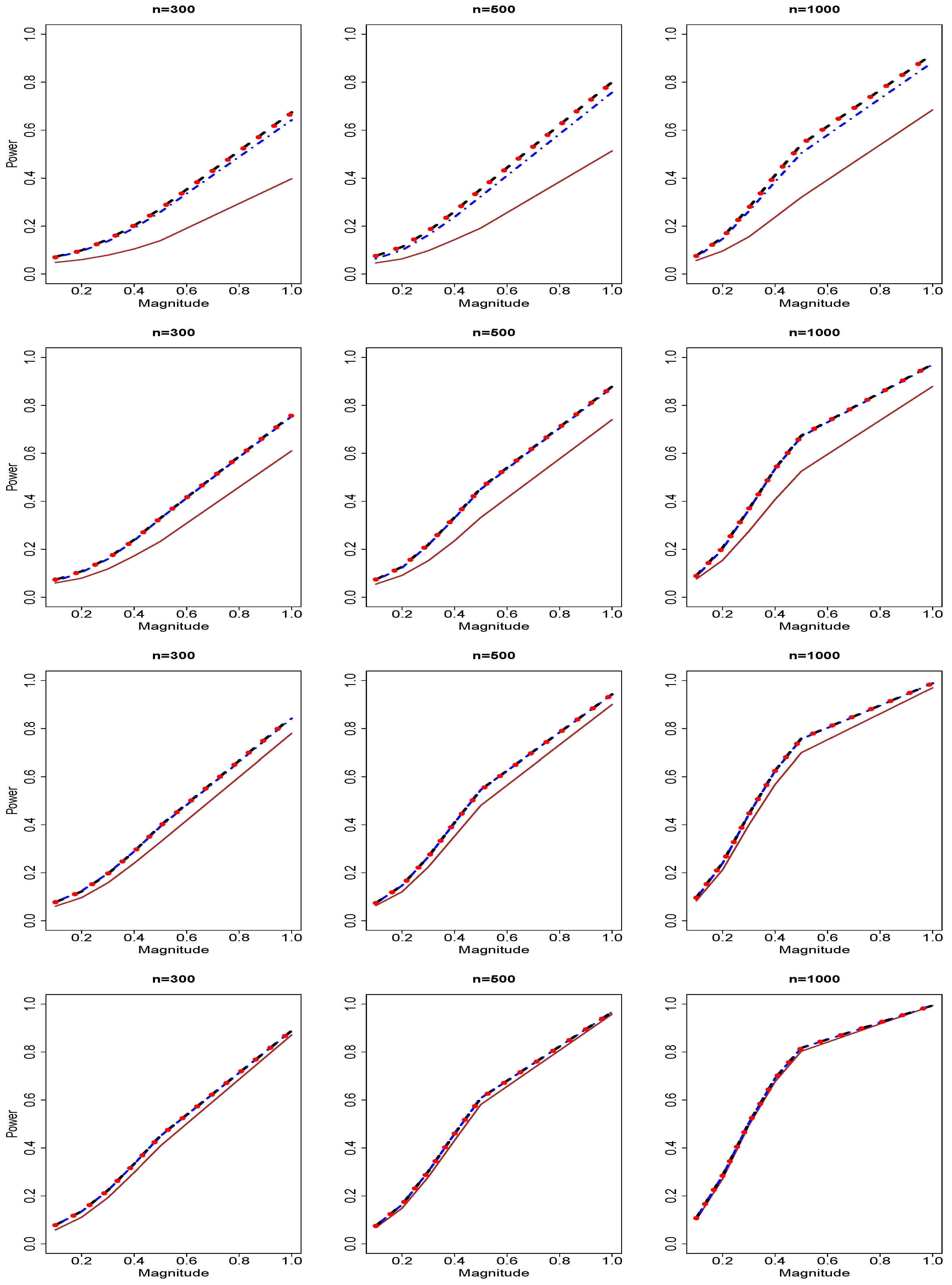
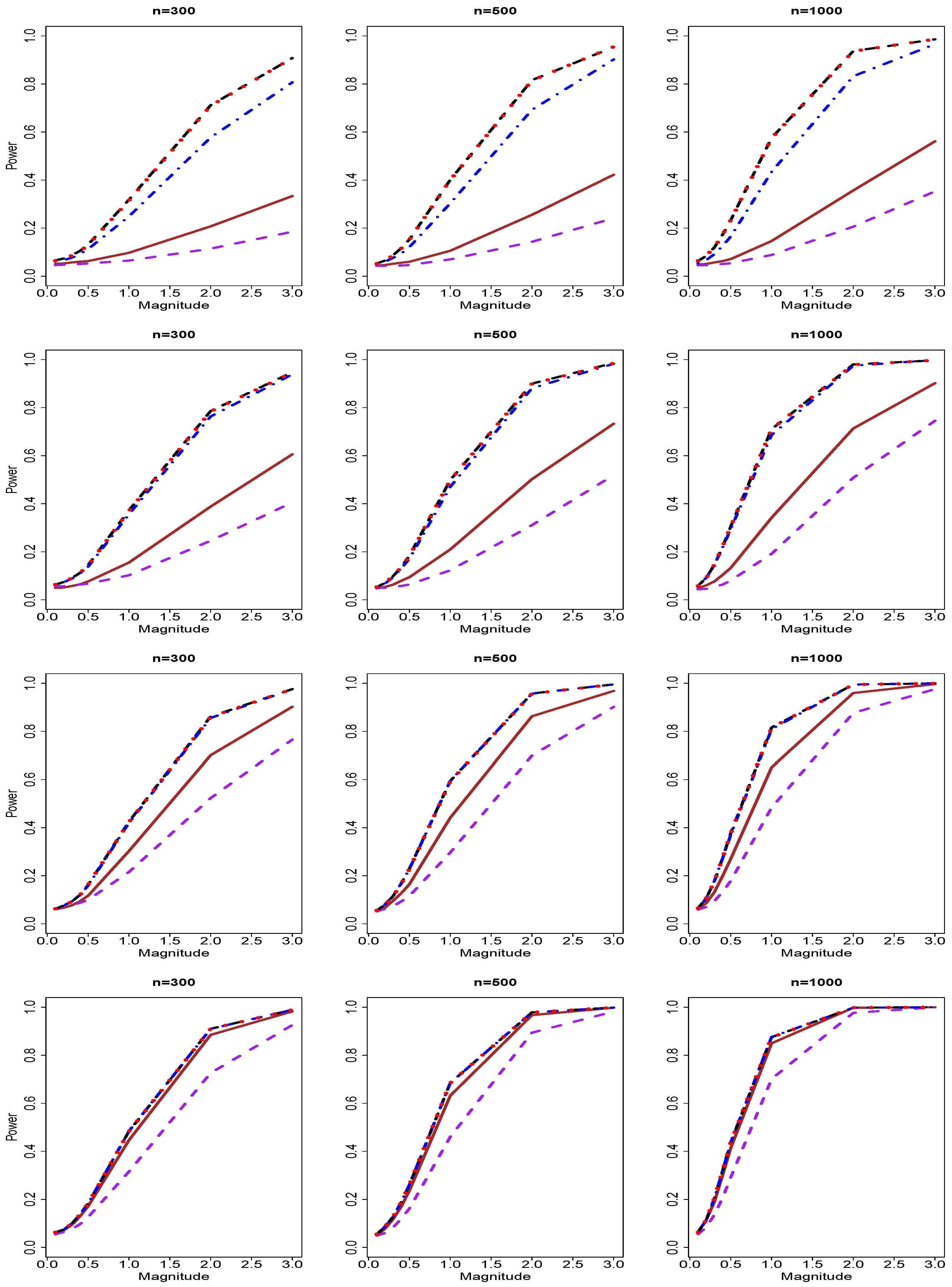
3.2. Results of Type II Errors and Power Analyses

We evaluate the performance of various methods from the perspective of statistical power. Type 2 error probability is the probability of accepting the null hypothesis when the truth is the alternative hypothesis, which is equal to one minus the statistical power, which is the probability of rejecting the null hypothesis when the truth is the alternative hypothesis.

In Figure 1, we report the power curves of tests for a group of common variants and a continuous phenotype. The four rows from top to bottom are for sequencing depths 1X, 2X, 4X and 10X. The three columns from left to right are for sample size n = 300, 500, 1000. The powers of the genotype-based F test (brown), NGS data-based joint significance test 1 (blue), test 2 (black) and test 3 (purple) are shown as curves in different colors. We found that in the low sequencing scenario (depth = 1X, 2X), there are advantages of NG data-based methods over the genotype-based F test. However, as the sequencing depth increases, the difference between the performance of sequencing data-based methods and the performance of genotype-based F test decreases. In the scenario of sequencing depth 10X, genotype-based methods are nearly the same or only slightly worse than NGS data-based methods. For all testing methods, we found increasing power as sample size increases or sequencing depth increases. Within the three NGS-data joint significance testing methods, NGS data-based joint significance test 3 (using sequencing data-based MLE of allele frequencies [30]) achieves nearly the same performance as NGS data-based Test 1 (using true allele frequencies). NGS data-based Test 2 (using a two-step genotype-based estimator of allele frequencies) has a relatively worse performance compared to Tests 1 and 3, but Test 2 is still better than their corresponding genotype-based methods. As sequencing depth increases, the difference between the performance of the three NGS data-based testing methods decreases.

In Figure 2, we report the power curve of tests for a group of rare genetic variants and continuous phenotypes. The four rows from top to bottom are for sequencing depths 1X, 2X, 4X and 10X. The three columns from left to right are for sample size n = 300, 500, 1000. The powers are of genotype-based burden test (brown), SKAT test (purple), NGS data-based variable collapse test 1 (black), test 2 (blue) and test 3 (red). We found that sequencing data-based methods are better than genotype-based methods in the scenarios of low sequencing depths (1X and 2X). As sequencing depth increases, the difference between the performance of genotype-based methods and sequencing data-based methods becomes smaller. For the scenario of sequencing depth 10X, the genotype-based burden test method and sequencing-based methods achieve similar performance. Within the three sequencing data-based variable collapse testing methods, Test 3 (estimate allele frequencies using a NGS data-based method) achieves nearly the same performance as Test 1 (using true allele frequencies). Test 2 (estimate allele frequencies using a two-step genotype-based method) is relatively worse compared to Tests 1 and 3. As sequencing depth increases, the difference between the performances of the three sequencing data-based methods disappears. Within the genotype-based methods, the burden test achieves better performance than SKAT methods because our scenarios assume all positive genetic effects that are not assumptions of SKAT, which allows both positive effects and negative effects.

We also conduct tests under the scenarios consistent with the assumptions of SKAT, i.e., genetic effects in both positive and negative directions, and find that burden tests, no matter whether they are genotype-based tests in the literature or NGS data-based tests proposed by us, fail as we expected because the burden test requires genetic effects to be only in one direction (positive or negative). The failure of the burden test under the scenarios for SKAT was recognized in the literature [21,26]. We leave the work of developing NGS data-based methods corresponding to genotype-based SKAT as our future study since it is beyond the scope of this article. The main objective of this article is to use a standard linear model framework to develop NGS data-based testing methods corresponding to genotype-based joint significance tests and genotype-based burden test in the literature.

3.3. Results of Estimating Allele Frequencies

Based on our simulated NGS data and corresponding true genotypes, we conducted genotype calling to obtain the estimated genotypes and then calculated allele frequency as a summary statistic based on estimated genotypes. We found that both genotype calling and allele frequency (a summary statistic) calculation based on estimated genotypes became more accurate when sequencing depth increased. To further evaluate the performance of estimators based on estimated genotypes versus estimators based on NGS data, we considered two allele-frequency estimators: (1) the two-step genotype-based estimation method, which first estimated genotypes based on sequencing data, and then estimated allele frequencies based on the estimated genotypes in the first step, and (2) the one-step sequencing data-based Maximum Likelihood Estimator (MLE) of allele frequencies. The use of the two estimation methods of allele frequencies and the use of true allele frequencies to deal with NGS data are proposed in Skotte et al., 2012 [30]. They stated that the one-step sequencing data-based method is better than the two-step genotype-based method in estimating allele frequencies [30]. In Table 3, we report the performance of the two estimators in terms of mean square error (MSE) and mean absolute deviation (MAD) for different sample sizes ($n=$ 300, 500, 1000) and different sequencing depths (1X, 2X, 4X, 10X). Denote $AF(i,j,k,l)$, $\widetilde{AF}(i,j,k,l)$ and $\widehat{AF}(i,j,k,l)$, respectively, as true allele frequency, estimated allele frequency using the two-step genotype-based method and estimated allele frequency using the one-step sequencing data-based method in sample size scenario i ($i=1,2,3$), sequencing depth scenario j ($j=1,2,3,4$), simulated NGS dataset k ($k=1,2,\cdots ,K$) and genetic variant l ($l=1,2,\cdots ,L$). MSE and MAD are calculated by the formulae

$$\begin{array}{ccc}\hfill MS{E}_1(i,j)& =& \sum _{k=1}^K\sum _{l=1}^L{\{\widetilde{AF}(i,j,k,l)-AF(i,j,k,l)\}}^2/(K\times L),\hfill \\ \hfill MS{E}_2(i,j)& =& \sum _{k=1}^K\sum _{l=1}^L{\{\widehat{AF}(i,j,k,l)-AF(i,j,k,l)\}}^2/(K\times L),\hfill \\ \hfill MA{D}_1(i,j)& =& \sum _{k=1}^K\sum _{l=1}^L|\widetilde{AF}(i,j,k,l)-AF(i,j,k,l)|/(K\times L),\hfill \\ \hfill MA{D}_2(i,j)& =& \sum _{k=1}^K\sum _{l=1}^L|\widehat{AF}(i,j,k,l)-AF(i,j,k,l)|/(K\times L),\hfill \end{array}$$

According to Table 3, we find that the one-step sequencing data-based estimator is better than the two-step genotype-based estimator in all 12 scenarios (all combinations of three sample sizes and four sequencing depths). The performance of both estimators improves with respect to an increase in sequencing depth or an increase in sample size.

4. Discussion

In this article, we adopted a standard linear model framework to derive NGS data-based testing methods for a group of common genetic variants and a group of rare genetic variants. The proposed methods are extensions of an NGS data-based testing method for a single genetic variant proposed by Skotte et al., 2012 [30] and Yan et al., 2015 [31]. With rapid advances in NGS technology and data, there is strong motivation to develop novel methods to deal with NGS data, preferably to have corresponding genotype-based methods in the literature for comparison. Since there are established methods for testing a group of common variants and a group of rare variants using genotypes in the literature, our proposed methods fill the literature gap by providing corresponding testing methods using sequencing data instead of the called genotypes.

We adopted a standard linear model framework and noticed that under the null hypothesis of no genetic effects, the likelihood function and its derivatives could be greatly simplified and easily calculated. Thus, we proposed a score test that only considers the evaluation of score functions and the information matrix at a constrained MLE, and the constrained MLE can be easily obtained. In this way, the chi-square statistic of our joint significance test is derived. Then, we apply the chain rule in calculus to derive our variable collapse test. We have provided full derivation details in the Appendix A, Appendix B, Appendix C, Appendix D and Appendix E.

There are different models to describe the genetic effects of a single marker with genotype g coded as 0, 1 and 2. Four widely-used genetic effect models are (1) additive model: $effect={\beta }_0+{\beta }_{a}g$, (2) dominant model: $effect={\beta }_0+{\beta }_{d}I(g\ge 1)$, (3) recessive model: $effect={\beta }_0+{\beta }_{r}I(g=2)$, (4) heterogeneous effect model: $effect={\beta }_0+{\beta }_{1}I(g=1)+{\beta }_{2}I(g=2)$, where $I(.)$ is the indicator function, which is equal to 1 when the condition specified in the parenthesis is satisfied, and 0 otherwise [51]. The phenotype modeled based on the dominant model, recessive model and heterogeneous effect model with $d_g$ genetic markers are, respectively,

$$\begin{array}{ccc}\hfill y_i& =& \alpha x_i^T+{\beta }_d{\left\{I(G_i\ge 1)\right\}}^T+{ϵ}_i={\eta }_i+{ϵ}_i,\hfill \\ \hfill y_i& =& \alpha x_i^T+{\beta }_a{\left\{I(G_i=2)\right\}}^T+{ϵ}_i={\eta }_i+{ϵ}_i,\hfill \\ \hfill y_i& =& \alpha x_i^T+{\beta }_1{\left\{I(G_i=1)\right\}}^T+{\beta }_2{I(G_i=2)}^T+{ϵ}_i={\eta }_i+{ϵ}_i,\hfill \end{array}$$

where ${\beta }_d$, ${\beta }_a$, ${\beta }_1$ and ${\beta }_2$ are the row vectors of length $d_g$, and ${\eta }_i$ is the linear predictor part. Although our proposed testing methods are described based on the additive model as described in Equation (7), the methods can be adapted to work for the other three genetic effects models by modifying the linear predictor ${\eta }_i$, and its first and second derivatives with respect to model parameters.

The main objective of this article is to apply standard statistical framework or mathematical statistics to develop novel methods to satisfy the need for group testing of common variants or rare variants based on next-generation data from the society of bioinformatics, biostatistics and modern biology. The proposed methods have a strict mathematical statistics foundation and show advantages over their corresponding genotype-based testing methods in the literature.

We only evaluated Type I errors (false positives) and Type II errors (false negatives) in our study. There are also other types of errors, including Type III errors involved in hypothesis testing. Type III errors refer to correctly rejecting the null hypothesis for the wrong reason. Other types of errors are also important in hypothesis testing, and future studies can be on other types of errors in addition to the widely-used evaluation of Type I errors and Type II errors.

Our proposed method is based on a linear model framework dealing with a continuous phenotype. In association studies, there are also other types of phenotypes, such as a binary phenotype, which is modeled as a logistic regression, and an integer phenotype (count data), which is modeled as a Poisson regression. In this article, our current methods are based on a standard linear model framework to handle a continuous phenotype. We aim to contribute to this area (NGS data-based association testing of a group of common variants or rare variants) by focusing on continuous phenotypes using a linear model framework. We are working on extending our methods to handle other types of phenotypes using a generalized linear model framework. A GLM framework-based derivation of testing methods to handle other types of phenotypes is feasible and under our development.

Sequencing depth plays an important role in the performance comparison of NGS data-based methods versus their corresponding genotype-based methods. When sequencing is deep, the genotype can be precisely called, and there are no big differences between the performances of sequencing data-based methods and their corresponding genotype-based methods. However, when the sequencing depth is not large (1X, 2X), genotypes can not be precisely called so that sequencing data-based methods can achieve better performance compared with their corresponding genotype-based methods [30,31]. Given the same budget constraint, a low sequencing depth with more individuals sequenced is preferred to a deep sequencing depth with few individuals sequenced [30,31]. Sequencing depths can also be different for different individuals. Future studies can be on NGS data-based association testing for individuals with heterogeneous sequencing depths.

5. Conclusions

We extend the NGS data-based methods to allow testing for a group of common variants or rare variants based on a linear model framework. Our proposed methods fill the literature gap and can achieve better performance compared with their corresponding genotype-based testing methods in the literature.

References

1. Men, A.E.; Wilson, P.; Siemering, K.; Forrest, S. Sanger DNA sequencing. In Next Generation Genome Sequencing: Towards Personalized Medicine; John Wiley & Sons: Hoboken, NJ, USA, 2008; pp. 1–11. [Google Scholar]
2. Illumina_Inc. DNA Sequencing with Solexa® Technology. Available online: https://courses.cs.duke.edu/spring21/compsci260/resources/GenomeSequencingTechnology/Illumina.Solexa.sequencing.pdf (accessed on 15 January 2023).
3. Wall, P.K.; Leebens-Mack, J.; Chanderbali, A.S.; Barakat, A.; Wolcott, E.; Liang, H.; Landherr, L.; Tomsho, L.P.; Hu, Y.; Carlson, J.E.; et al. Comparison of next generation sequencing technologies for transcriptome characterization. BMC Genom. 2009, 10, 347. [Google Scholar] [CrossRef] [PubMed] [Green Version]
4. Mardis, E.R. Next-generation sequencing platforms. Annu. Rev. Anal. Chem. 2013, 6, 287–303. [Google Scholar] [CrossRef] [PubMed] [Green Version]
5. Shendure, J.; Ji, H. Next-generation DNA sequencing. Nat. Biotechnol. 2008, 26, 1135–1145. [Google Scholar] [CrossRef]
6. Liu, L.; Li, Y.; Li, S.; Hu, N.; He, Y.; Pong, R.; Lin, D.; Lu, L.; Law, M. Comparison of next-generation sequencing systems. J. Biomed. Biotechnol. 2012, 2012, 251364. [Google Scholar] [CrossRef]
7. Long, K.; Cai, L.; He, L. DNA sequencing data analysis. In Computational Systems Biology; Springer: Berlin/Heidelberg, Germany, 2018; pp. 1–13. [Google Scholar]
8. Van der Auwera, G.A.; Carneiro, M.O.; Hartl, C.; Poplin, R.; Del Angel, G.; Levy-Moonshine, A.; Jordan, T.; Shakir, K.; Roazen, D.; Thibault, J.; et al. From FastQ data to high-confidence variant calls: The genome analysis toolkit best practices pipeline. Curr. Protoc. Bioinform. 2013, 43, 11.10.1–11.10.33. [Google Scholar] [CrossRef] [Green Version]
9. Moore, J.H.; Asselbergs, F.W.; Williams, S.M. Bioinformatics challenges for genome-wide association studies. Bioinformatics 2010, 26, 445–455. [Google Scholar] [CrossRef] [Green Version]
10. Nielsen, R.; Paul, J.S.; Albrechtsen, A.; Song, Y.S. Genotype and SNP calling from next-generation sequencing data. Nat. Rev. Genet. 2011, 12, 443–451. [Google Scholar] [CrossRef] [Green Version]
11. Liu, Q.; Guo, Y.; Li, J.; Long, J.; Zhang, B.; Shyr, Y. Steps to ensure accuracy in genotype and SNP calling from Illumina sequencing data. BMC Genom. 2012, 13, S8. [Google Scholar] [CrossRef] [Green Version]
12. Nielsen, R.; Korneliussen, T.; Albrechtsen, A.; Li, Y.; Wang, J. SNP calling, genotype calling, and sample allele frequency estimation from new-generation sequencing data. PLoS ONE 2012, 7, e37558. [Google Scholar] [CrossRef] [Green Version]
13. Lewis, C.M.; Knight, J. Introduction to Genetic Association Studies; CSHL Press: Cold Spring Harbor, NY, USA, 2012; Volume 2012. [Google Scholar] [CrossRef] [Green Version]
14. Balding, D.J. A tutorial on statistical methods for population association studies. Nat. Rev. Genet. 2006, 7, 781–791. [Google Scholar] [CrossRef]
15. Huang, E.; Aitken, K.; George, A. Association studies. In Genetics, Genomics and Breeding of Sugarcane; CRC Press: Boca Raton, FL, USA, 2010; pp. 43–68. [Google Scholar]
16. Cordell, H.J.; Clayton, D.G. Genetic association studies. Lancet 2005, 366, 1121–1131. [Google Scholar] [CrossRef] [PubMed]
17. Lee, S.; Abecasis, G.R.; Boehnke, M.; Lin, X. Rare-variant association analysis: Study designs and statistical tests. Am. J. Hum. Genet. 2014, 95, 5–23. [Google Scholar] [CrossRef] [PubMed] [Green Version]
18. Via, M.; Gignoux, C.; Burchard, E.G. The 1000 Genomes Project: New opportunities for research and social challenges. Genome Med. 2010, 2, 3. [Google Scholar] [CrossRef] [PubMed] [Green Version]
19. Luo, L.; Boerwinkle, E.; Xiong, M. Association studies for next-generation sequencing. Genome Res. 2011, 21, 1099–1108. [Google Scholar] [CrossRef] [PubMed] [Green Version]
20. Galesloot, T.E.; Van Steen, K.; Kiemeney, L.A.; Janss, L.L.; Vermeulen, S.H. A comparison of multivariate genome-wide association methods. PLoS ONE 2014, 9, e95923. [Google Scholar] [CrossRef] [PubMed]
21. Wang, Y.T.; Sung, P.Y.; Lin, P.L.; Yu, Y.W.; Chung, R.H. A multi-SNP association test for complex diseases incorporating an optimal P-value threshold algorithm in nuclear families. BMC Genom. 2015, 16, 381. [Google Scholar] [CrossRef] [PubMed] [Green Version]
22. Auer, P.L.; Lettre, G. Rare variant association studies: Considerations, challenges and opportunities. Genome Med. 2015, 7, 16. [Google Scholar] [CrossRef] [Green Version]
23. Liu, D.J.; Leal, S.M. A novel adaptive method for the analysis of next-generation sequencing data to detect complex trait associations with rare variants due to gene main effects and interactions. PLoS Genet. 2010, 6, e1001156. [Google Scholar] [CrossRef] [Green Version]
24. Lin, W.Y. Beyond rare-variant association testing: Pinpointing rare causal variants in case-control sequencing study. Sci. Rep. 2016, 6, 21824. [Google Scholar] [CrossRef] [Green Version]
25. Zhao, J.; Akinsanmi, I.; Arafat, D.; Cradick, T.; Lee, C.M.; Banskota, S.; Marigorta, U.M.; Bao, G.; Gibson, G. A burden of rare variants associated with extremes of gene expression in human peripheral blood. Am. J. Hum. Genet. 2016, 98, 299–309. [Google Scholar] [CrossRef] [Green Version]
26. Wu, M.C.; Lee, S.; Cai, T.; Li, Y.; Boehnke, M.; Lin, X. Rare-variant association testing for sequencing data with the sequence kernel association test. Am. J. Hum. Genet. 2011, 89, 82–93. [Google Scholar] [CrossRef] [PubMed] [Green Version]
27. Lee, S.; Wu, M.C.; Lin, X. Optimal tests for rare variant effects in sequencing association studies. Biostatistics 2012, 13, 762–775. [Google Scholar] [CrossRef] [Green Version]
28. Plagnol, V.; Cooper, J.D.; Todd, J.A.; Clayton, D.G. A method to address differential bias in genotyping in large-scale association studies. PLoS Genet. 2007, 3, e74. [Google Scholar] [CrossRef] [PubMed] [Green Version]
29. Sham, P.C.; Purcell, S.M. Statistical power and significance testing in large-scale genetic studies. Nat. Rev. Genet. 2014, 15, 335–346. [Google Scholar] [CrossRef] [PubMed]
30. Skotte, L.; Korneliussen, T.S.; Albrechtsen, A. Association testing for next-generation sequencing data using score statistics. Genet. Epidemiol. 2012, 36, 430–437. [Google Scholar] [CrossRef]
31. Yan, S.; Yuan, S.; Xu, Z.; Zhang, B.; Zhang, B.; Kang, G.; Byrnes, A.; Li, Y. Likelihood-based complex trait association testing for arbitrary depth sequencing data. Bioinformatics 2015, 31, 2955–2962. [Google Scholar] [CrossRef] [Green Version]
32. Harismendy, O.; Ng, P.C.; Strausberg, R.L.; Wang, X.; Stockwell, T.B.; Beeson, K.Y.; Schork, N.J.; Murray, S.S.; Topol, E.J.; Levy, S.; et al. Evaluation of next generation sequencing platforms for population targeted sequencing studies. Genome Biol. 2009, 10, R32. [Google Scholar] [CrossRef] [Green Version]
33. Li, Y.; Chen, W.; Liu, E.Y.; Zhou, Y.H. Single nucleotide polymorphism (SNP) detection and genotype calling from massively parallel sequencing (MPS) data. Stat. Biosci. 2013, 5, 3–25. [Google Scholar] [CrossRef] [Green Version]
34. Huang, H.; Chanda, P.; Alonso, A.; Bader, J.S.; Arking, D.E. Gene-based tests of association. PLoS Genet. 2011, 7, e1002177. [Google Scholar] [CrossRef] [Green Version]
35. Weir, B.S. Genetic Data Analysis II; Sinauer Associates: Sunderland, MA, USA, 1996. [Google Scholar]
36. Davey, J.W.; Hohenlohe, P.A.; Etter, P.D.; Boone, J.Q.; Catchen, J.M.; Blaxter, M.L. Genome-wide genetic marker discovery and genotyping using next-generation sequencing. Nat. Rev. Genet. 2011, 12, 499–510. [Google Scholar] [CrossRef]
37. Li, Y.; Willer, C.J.; Ding, J.; Scheet, P.; Abecasis, G.R. MaCH: Using sequence and genotype data to estimate haplotypes and unobserved genotypes. Genet. Epidemiol. 2010, 34, 816–834. [Google Scholar] [CrossRef] [PubMed] [Green Version]
38. Hong, H.; Xu, L.; Su, Z.; Liu, J.; Ge, W.; Shen, J.; Fang, H.; Perkins, R.; Shi, L.; Tong, W. Pitfall of genome-wide association studies: Sources of inconsistency in genotypes and their effects. J. Biomed. Sci. Eng. 2012, 5, 23768. [Google Scholar] [CrossRef] [Green Version]
39. Yan, S.; Li, Y. BETASEQ: A powerful novel method to control type-I error inflation in partially sequenced data for rare variant association testing. Bioinformatics 2014, 30, 480–487. [Google Scholar] [CrossRef] [PubMed] [Green Version]
40. Korneliussen, T.S.; Albrechtsen, A.; Nielsen, R. ANGSD: Analysis of next generation sequencing data. BMC Bioinform. 2014, 15, 356. [Google Scholar] [CrossRef] [Green Version]
41. Belonogova, N.M.; Svishcheva, G.R.; Axenovich, T.I. FREGAT: An R package for region-based association analysis. Bioinformatics 2016, 32, 2392–2393. [Google Scholar] [CrossRef]
42. Agresti, A. Categorical Data Analysis; Wiley Series in Probability and Statistics; Wiley: Hoboken, NJ, USA, 2013. [Google Scholar]
43. McCullagh, P.; Nelder, J. Generalized Linear Models, 2nd ed.; Chapman & Hall: London, UK, 1989. [Google Scholar]
44. Baxter, M. Generalised linear models, by P. McCullagh and JA Nelder. Pp 511.£ 30. 1989. ISBN 0-412-31760-5 (Chapman and Hall). Math. Gaz. 1990, 74, 320–321. [Google Scholar] [CrossRef]
45. Cox, D.R. Principles of Statistical Inference; Cambridge University Press: Cambridge, UK, 2006. [Google Scholar]
46. Young, G.A.; Smith, R.L. Essentials of Statistical Inference; Cambridge University Press: Cambridge, UK, 2005; Volume 16. [Google Scholar]
47. Sul, J.H.; Han, B.; He, D.; Eskin, E. An optimal weighted aggregated association test for identification of rare variants involved in common diseases. Genetics 2011, 188, 181–188. [Google Scholar] [CrossRef] [Green Version]
48. Ionita-Laza, I.; Buxbaum, J.D.; Laird, N.M.; Lange, C. A new testing strategy to identify rare variants with either risk or protective effect on disease. PLoS Genet. 2011, 7, e1001289. [Google Scholar] [CrossRef] [Green Version]
49. Schaffner, S.F.; Foo, C.; Gabriel, S.; Reich, D.; Daly, M.J.; Altshuler, D. Calibrating a coalescent simulation of human genome sequence variation. Genome Res. 2005, 15, 1576–1583. [Google Scholar] [CrossRef] [Green Version]
50. Kang, J.; Huang, K.C.; Xu, Z.; Wang, Y.; Abecasis, G.R.; Li, Y. AbCD: Arbitrary coverage design for sequencing-based genetic studies. Bioinformatics 2013, 29, 799–801. [Google Scholar] [CrossRef] [Green Version]
51. Liu, H.M.; Zheng, J.P.; Yang, D.; Liu, Z.F.; Li, Z.; Hu, Z.Z.; Li, Z.N. Recessive/dominant model: Alternative choice in case-control-based genome-wide association studies. PLoS ONE 2021, 16, e0254947. [Google Scholar] [CrossRef] [PubMed]
Figure 1. Power Curves of Tests for a Group of Common Genetic Variants and Continuous Phenotype. The four rows of images from up to down are for sequencing depths 1X, 2X, 4X and 10X. The three columns of images from left to right are for sample size n = 300 , 500 , 1000 . Powers of genotype-based F test (brown solid line), NGS data-based joint significance test 1 (black dashed line), test 2 (blue dashed dotted line) and test 3 (red dotted line).
Mathematics 11 01285 g001
Figure 2. Power Curves of Tests for a Group of Rare Genetic Variants and Continuous Phenotype. The four rows of images from up to down are for sequencing depths 1X, 2X, 4X and 10X. The three columns of images from left to right are for sample size n = 300 , 500 , 1000 . Powers of genotype-based burden test (brown solid line), genotype-based SKAT test (purple dashed line), NGS data-based variable collapse test 1 (black dashed line), test 2 (blue dashed dotted line) and test 3 (red dotted line).
Mathematics 11 01285 g002