Article

A Dynamic Competition Analysis of Stochastic Fractional Differential Equation Arising in Finance via Pseudospectral Method

1
Department of Mathematics and Statistics, College of Science, King Faisal University, P.O. Box 400, Al-Ahsa 31982, Saudi Arabia
2
Department of Mathematics, City University of Science and Information Technology, Peshawar 2500, KP, Pakistan
*
Author to whom correspondence should be addressed.
Mathematics 2023, 11(6), 1328; https://doi.org/10.3390/math11061328
Submission received: 15 February 2023 / Revised: 7 March 2023 / Accepted: 8 March 2023 / Published: 9 March 2023
(This article belongs to the Section Difference and Differential Equations)

Abstract

:
This research focuses on the analysis of the competitive model used in the banking sector based on the stochastic fractional differential equation. For the approximate solution, a pseudospectral technique is utilized for the proposed model based on the stochastic Lotka–Volterra equation using a wide range of fractional order parameters in simulations. Conditions for stable and unstable equilibrium points are provided using the Jacobian. The Lotka–Volterra equation is unstable in the long term and can produce highly fluctuating dynamics, which is also one of the reasons that this equation is used to model the problems arising in finance, where fluctuations are important. For this reason, the conventional analytical and numerical methods are not the best choices. To overcome this difficulty, an automatic procedure is used to solve the resultant algebraic equation after the discretization of the operator. In order to fully use the properties of orthogonal polynomials, the proposed scheme is applied to the equivalent integral form of stochastic fractional differential equations under consideration. This also helps in the analysis of fractional differential equations, which mostly fall in the framework of their integrated form. We demonstrate that this fractional approach may be considered as the best tool to model such real-world data situations with very reasonable accuracy. Our numerical simulations further demonstrate that the use of the fractional Atangana–Baleanu operator approach produces results that are more precise and flexible, allowing individuals or companies to use it with confidence to model such real-world situations. It is shown that our numerical simulation results have a very good agreement with the real data, further showing the efficiency and effectiveness of our numerical scheme for the proposed model.

1. Introduction

Due to their ability to capture the exact description of some real-world phenomena, fractional calculus is attracting a great deal of attention from researchers, especially in engineering and applied sciences. Most recently, the application of this to the investigation of a dynamical system’s differential equations of fractional order has gained more popularity. This is due to the fact that these models allow a significant amount of freedom. This quality of fractional differential equations makes them the most suitable candidate for analyzing the data in the banking sector. In the banking sector, the subsidiary bank receives capital from the mother bank, which is further distributed between individuals or companies. Financial institutions such as banks are actively involved in granting loans and in stock markets. They play the role of an interface between companies or individuals. As the marketplace is very competitive, in general, this type of behavior is described using Lotka–Volterra stochastic models of fractional order. Banks are also defined as commercial establishments that take deposits from people of a given geographic region, with the goal of investing those funds in public initiatives that will better the quality of life of those persons. Banks may do more than simply accept deposits and lend money; they can also be a potent tool for the promotion of economic growth and the preservation of social harmony. Specifically, rural and commercial banks contribute to various sorts of economic growth efforts. Commercial banks are financial entities that execute financial transactions in conformity with Syariah standards. Some banks that provide both traditional and Islamic banking services operate in conformity with the principles of both systems [1].
Commercial banks have a responsibility to defend the public and economic growth by funding national development projects. According to Act No. 10 from 1998 in Indonesia, a rural bank is one that does not engage in payment traffic and whose operations are in accordance with Shariah principles or conventional banking standards [2]. Rural banks only collect public funds on time deposits, savings, and credit and deposit money in the form of Bank Certificates, as opposed to commercial banks, who also participate in payment traffic, currency production, and equity participation. In countries with more rural banks than city banks, in light of the wider scope of activities undertaken by commercial banks, stricter capital requirements are imposed on the city banks for high profits, while rural banks specialize in a narrower range of activities, resulting in lower profits. Rural banks suffer from a lack of both customers and profits, while urban banks enjoy a great deal of both. Customers may try to find the best deal by shopping around, as there is not much of a difference between the two banks’ offerings.
If it is anticipated that commercial and rural banks would be pitted against one another in a competitive market, then the Lotka–Volterra competition models, initially published in 1920 by Alfred J. Lotka and Vito Volterra, may be used to examine the dynamic behavior of the sector. In order to model the competition for food and other limited resources, two equations are utilized. This model generalizes the logistics model so that it may be used to make more precise predictions in competitive settings involving several species. The Lotka–Volterra model has been used in research by a variety of academics [3,4]. For instance, the competitive model is applied using information from Korean mobile providers. The transition from one technology to another is seen as a contest. Stock market, market dynamics, modeling, and policy implications are only some of the topics that have been studied in depth in several studies [5,6]. Consequences for the nation are one of the many issues that arise from these discussions; we refer the reader to the latest studies on a competition model for financial data [7].
The Lotka–Voltera model, also known as the prey–predator model, consists of a system of differential equations that are nonlinear in nature. In the early days after introducing this model, it was mostly used in applications in mathematical biology, where it was used for the interaction between dynamic species that are different in nature. After its publication, many authors used it in many other applications. For example, in the field of finance and economics, it is used in the banking system, where it is used to study the dynamics and the relation between loan and deposit growth in the balance sheets of banks and their capital structure. The predator entity is used as a loan, while the deposit is used as prey. The allocation of the loan totally depends on deposits. The more deposits there are, the more the bank will give loans. In most of these studies in the banking sector, the deterministic version of this model has been widely used mostly. In general, the loan and deposit entities are stochastic; therefore, in their interactions, they may occur as random noise. Therefore, it is more natural to use the stochastic version of the proposed model instead of its deterministic counterpart. The stochastic model based on Lotka–Voltera has been used by many researchers to study the applications of some physical world problems. For example, the prey model application is used in random environmental situation in [8]. A numerical scheme based on the method of Euler–Maruyama has been investigated to see the dynamics of loan and deposit volume, and the author uses the least-square scheme for the estimation of parameters [9]. A fractional order model equation based on the Lotka–Voltera system has the advantage of generating fractional Brownian motion, which is not only Gaussian in nature but also non-Markovian in general. These fractional order models also provide a great degree of freedom, which is very important in the research field of chaos.
Most of these models have been investigated in the context of the integer-order scenario. Researchers turn to fractional calculus while trying to describe the dynamics of a particle event using a standard integer-order explanation. Since fractional calculus can be used in many different mathematical models in science and engineering, it has attracted a great deal of attention from experts in these fields. This is because the usefulness of the fractional operators may be explored in many settings using fractional calculus. Caputo, Caputo–Fabrizio, and Atangana–Baleanu are three fractional operators that see frequent application in current academic work. The Caputo and Caputo–Fabrizio versions may not have been sufficient for real-world challenges since they rely on a single kernel. Researchers built a model using this set of operators and other sets of operators and then compared it to data collected in the real world to get the most precise description of the model and the most accurate estimate of its parameters [10,11]. The studies into various models were aided by the data presented in the aforementioned publications. Recently, a growing number of more sophisticated fractional mathematical models and their applications have been developed in a variety of industrial and scientific fields [12,13,14].
Recently, an advection–dispersion model equation of fractional order in the space Caputo derivatives sense has been investigated numerically by using a finite difference scheme in compact form for time coordinates, while Chebyshev polynomials of the fourth kind are used for the discretization of a special part in [15], while a computational scheme for differential equations of fractional order in time was derived and investigated theoretically by the authors in [16]. A fractional order equation consists of autonomous differential equations of ordinary type with non-singular kernels using graphical and analytical as well as numerical methods [17]. Tayyaba et.al used a numerical method consisting of B-spline cubic approximation for the Fisher equation of fractional order in time in [18]. For details about the theory of fractional order differential equations, we refer the reader to the monographs [19,20].
A fractional model is presented for the banking data in a recent study that uses the framework created by Atangana–Baleanu and its derivation by Caputo by utilizing a wider range of CF operators and least-squares curve fitting to generate model parameters in [21]. In the current work, in addition to using Caputo, CF, and AB’s derivative, we revised the data by using their fractional parameter model in the sense of Caputo, CF, and AB [22,23], using fractional calculus to extrapolate results from real-world data by varying its types. Some of the studies related to the applications of some infectious diseases have also been investigated using the optimal control with fractional differential equations and higher-order schemes in [24,25,26,27,28,29,30,31]. We designed and executed an investigation of real data using a broad range of fractional approaches. We have also included a survey of relevant subjects related to the planned study and a detailed literature evaluation of fraction calculus’s practical applications. For numerical simulations, we use a higher-order numerical scheme based on Legendre orthogonal polynomials [32,33,34,35,36,37,38,39].
The main purpose of this research work is to investigate the fractional order stochastic model based on the system of Lotka–Voltera model equations both theoretically and numerically. To this end, we use a more reliable and efficient numerical scheme based on the Legendre collocation method, which has an exponential convergence rate for smooth data.
The layout of the rest of the this paper is organized as follows. In Section 2, a mathematical model is formulated, and the proposed methodology is discussed in detail. Section 3 consists of some basics of fractional calculus that are necessary for the detail analysis of the proposed model. The numerical results are described in Section 4, while the conclusion is drawn in Section 5.

2. Model Formulation and Method Description

To mathematically formulate the model, the Lotka–Volterra model is fitted to the top-profit data using the least-squares approach. There seem to be two unique flavors of the Lotka–Volterra model: x for commercial bank profits and y for rural bank profits. Some of the assumptions used while creating models are listed below:
It was anticipated that the increase in the number of banks could be accommodated logistically.
There is not much difference between the commercial and rural banking sectors in terms of yearly profit.
In order to simulate the connection between urban and rural financial institutions, we may utilize the following set of ordinary differential equations. This modeling relies on the above assumptions.
d x ( t ) d t = r 1 x 1 x ( t ) p 1 β 1 x ( t ) y ( t ) d y ( t ) d t = r 2 y 1 y ( t ) p 2 β 2 x ( t ) y ( t ) ,
where the positive initial conditions are x ( 0 ) = x 0 and y ( 0 ) = y 0 , and also r 1 and r 2 are the pace of growth in commercial banks’ and rural banks’ profits. p 1 represents the maximum possible profit for the commercial bank, whereas p 2 represents the highest possible profit for the rural bank. Coefficients for commercial banks are represented by the parameter β 1 , while those for rural banks are represented by the parameter β 2 . In the provided model system Equation (1), the unknown parameters are r i , p i and β i for i = 1 , 2 . We show several interesting applications of these operators for data fitting and find the best possible fit using the least squares approach for curve fitting, followed by the use of fractional operators such as the Atangana–Baleanu (AB) method for the proposed system in Equation (1).
d x ( t ) d t = r 1 x 1 x ( t ) p 1 β 1 x ( t ) y ( t ) + σ x ( t ) d W ( t ) d t , d y ( t ) d t = r 2 y 1 y ( t ) p 2 β 2 x ( t ) y ( t ) + σ y ( t ) d W ( t ) d t ,
where σ is intensity of Brownian motion W ( t ) . To discuss and solve the given systems using the proposed scheme, we first briefly provide an overview of the Legendre polynomials. Let Q n ( τ a ) signify the Legendre polynomials of nth order. The function g ( τ a ) given on the interval 1 , 1 is approximated by
g ( τ a ) = i = 0 n g i Q i ( τ a )
X i = g ( τ a i ) represents the undetermined Legendre coefficients, τ a i , i = 0 , 1 , , n represents a point set satisfying an interpolation 1 = τ a 0 < τ a 1 < < τ a n = 1 , and Q n ( τ a ) indicates the nth power or degree. We may write the Legendre polynomial as
Q i ( τ a ) = 1 2 i a = 0 [ i 2 ] ( 1 ) a ( a i ) ( i 2 i 2 a ) τ i 2 a , τ a 1 , 1 i = 0 , 1 , 2 , , n
i 2 = i 2 , i f i Even , i 1 2 , i f i Odd .
The stochastic bank data model given Equation (2) is solved using the Legendre pseudospectral using the following steps, which is based on the Lagendre–Gauss quadrature with weight function. Specifically, the Legendre–Gauss–Lobato points denoted by { t j } j = 0 N , of the form t j = cos ( j π N + 1 ) for 0 n N were used. To get a numerical answer to Equation (2), we first integrate from [ 0 , t ] of Equation (2), which takes the form
x ( t ) = x ( 0 ) + 0 t r 1 x 1 x ( s ) p 1 β 1 x ( s ) y ( s ) d s + 0 t σ x ( s ) d W ( s ) , y ( t ) = y ( 0 ) + 0 t r 2 y 1 y ( s ) p 2 β 2 x ( s ) y ( s ) d s + 0 t σ y ( s ) d W ( s ) ,
where the functions x ( t ) and y ( t ) have their starting values x ( 0 ) and y ( 0 ) . Taking linear transformations into account, we conduct an investigation of the Legendre spectral collocation technique on the interval [ 1 , 1 ] . s = t 2 ( θ + 1 ) , then Equation (5) becomes
x ( t ) = x ( 0 ) + t 2 1 1 r 1 x 1 x t 2 ( θ + 1 ) p 1 β 1 x t 2 ( θ + 1 ) y t 2 ( θ + 1 ) d θ + t 2 1 1 σ x t 2 ( θ + 1 ) d W ( θ ) , y ( t ) = y ( 0 ) + t 2 1 1 r 2 y 1 y t 2 ( θ + 1 ) p 2 β 2 x t 2 ( θ + 1 ) y t 2 ( θ + 1 ) d θ + t 2 1 1 σ y t 2 ( θ + 1 ) d W ( θ ) ,
The semi-discretized spectral equations of Equation (6) are
x ( t ) = x ( 0 ) + t 2 k = 0 N r 1 x 1 x t 2 ( θ + 1 ) p 1 β 1 x t 2 ( θ + 1 ) y t 2 ( θ + 1 ) w k + t 2 k = 0 N σ x t 2 ( θ + 1 ) w k * , y ( t ) = y ( 0 ) + t 2 k = 0 N r 2 y 1 y t 2 ( θ + 1 ) p 2 β 2 x t 2 ( θ + 1 ) y t 2 ( θ + 1 ) w k + t 2 k = 0 N σ y t 2 ( θ + 1 ) w k * ,
where the Legendre weight function is given by
ω k = 2 ( 1 s k 2 ) [ L N + 1 ( s k ) ] 2 , 0 k N .
Similarly, the stochastic Legendre weight function is
ω k * = ω k × r a n d n ( 1 , N ) , 0 k N .
After that, we use Legendre polynomials to approximate the solution to Equation (2) for each class; the same procedure is used for Equation (3):
x ( t ) = n = 0 N x n P n ( t ) , y ( t ) = n = 0 N y n P n ( t ) ,
where the Legendre coefficients for the function x ( t ) and y ( t ) are denoted by x n and y n , respectively. Now, applying the approximation obtained earlier in Equation (7),
n = 0 N x n P n ( t ) = n = 0 N x n P n ( 0 ) + t 2 k = 0 N { r 1 n = 0 N x n P n 1 n = 0 N x n P n η k p 1 β 1 n = 0 N x n P n ( η k ) n = 0 N y n P n ( η k ) } w k + t 2 k = 0 N σ n = 0 N x n P n ( η k ) w k * , n = 0 N y n P n ( t ) = n = 0 N y n P n ( 0 ) + t 2 k = 0 N { r 2 n = 0 N y n P n 1 n = 0 N y n P n η k p 2 β 2 n = 0 N x n P n ( η k ) n = 0 N y n P n ( η k ) } w k + t 2 k = 0 N σ n = 0 N y n P n ( η k ) w k * ,
where for simplification we take η k = t 2 ( θ + 1 ) .
Therefore, the system in Equation (9) contains 2 N + 2 number of unknown concerns with 2 N nonlinear algebraic equations, in accordance with the initial conditions:
n = 0 N x n P n ( 0 ) = ν 1 , n = 0 N y n P n ( 0 ) = ν 2 ,
Therefore, Equation (10) along with Equation (9) form a system of ( 2 N + 2 ) nonlinear equations with the same number of unknowns. From the above system, we obtained the unknowns x n , y n , by putting the values of unknowns in Equation (8) and obtained the numerical solution to the stochastic system given in Equation (2). Here, we omit the solution procedure to the model Equation (1), as its solution procedure is same as for the model Equation (2) by deleting the last term in each step of Equation (2).
For parameter estimation, in order to estimate the unobserved model parameters, we use the strategy given by the authors using the statistics database that includes data from 2004 through 2014 given in [21] and the citations therein. The information is collected from commercial and rural banks, and the banks’ annual profits serve as the primary metric by which we rank them. The results of a practice session on curve fitting are obtained using the least squares approach. Our findings from the commercial bank against the actual data utilizes data gathered through curve fitting to compare the rural and commercial bank using the proposed model.

3. Basics of Fractional Calculus

In this section, we go through the fractional derivatives in the form of definitions related to fractional models. We also state some theoretical results in the form of theorems that are useful to support the numerical simulations. We provide three frequently used fractional operators: we look into Caputo, Caputo–Fabrizio, and Atangana–Baleanu derivatives [40].
Definition 1.
Let a function u : R + R with fractional order α > 0 ; then, one can define the fractional integral of order α > 0 as follows:
I t α ( u ( t ) ) = 1 Γ ( α ) 0 t ( t s ) α 1 u ( s ) d s
where Γ describes the Gamma function and α shows the fractional order parameter.
Definition 2.
Consider u H 1 ( f , g ) , with f < g , and α [ 0 , 1 ] ; then, we define the Atangana–Baleanu derivative in the following:
A B 0 D t α u ( t ) = P ( α ) 1 α a t u ( s ) E α [ α 1 α ( t s ) α ] d s
Definition 3.
Here is a formula for the fractional integral of the Atangana–Baleanu derivative:
A B a I t α u ( t ) = 1 α ρ ( α ) u ( t ) + α ρ ( α ) Γ ( α ) 0 t f ( s ) ( t s ) α 1 d s
When this occurs, the case of the original function is restored as a = 0 .

3.1. Atangana–Baleanu Fractional Model

The system that results from applying the Atangana–Baleanu derivative definition to the model is known as the Atangana–Baleanu fractional model, which tends to the following system:
A B 0 D t α x ( t ) = r 1 x ( 1 x ( t ) p 1 ) β 1 x ( t ) y ( t ) A B 0 D t α y ( t ) = r 2 y ( 1 y ( t ) p 2 ) β 2 x ( t ) y ( t ) ,
and specifically, the Atangana–Baleanu model’s fractional parameter is written as
A B 0 D t α x ( t ) = r 1 α x ( 1 x ( t ) p 1 α ) β 1 x ( t ) y ( t ) A B 0 D t α y ( t ) = r 2 α y ( 1 y ( t ) p 2 α ) β 2 x ( t ) y ( t )
In the next part, we update the numerical solution to systems of Equations (13) and (14) and compare the computational and experimental outcomes.

3.2. Equilibria and Their Stability

The following is the method for obtaining the equilibrium points for the model in Equation (13) under consideration:
A B 0 D t α x ( t ) = 0 , A B 0 D t α y ( t ) = 0 ;
using the above, Equation (13) takes the form
r 1 x 1 x ( t ) p 1 β 1 x ( t ) y ( t ) = 0 r 2 y 1 y ( t ) p 2 β 2 x ( t ) y ( t ) = 0 ;
Solving the equations in Equation (16), we have
E 0 = ( 0 , 0 ) , E 1 = ( 0 , p 2 ) , E 2 = ( p 1 , 0 ) , E 3 = r 1 p 1 ( p 2 β 1 r 1 ) p 1 p 2 β 1 β 2 r 1 r 2 , r 2 p 2 ( p 1 β 2 r 2 ) p 1 p 2 β 1 β 2 r 1 r 2
These stable equilibrium points may be used to draw inferences about the system’s equations in Equation (13). The Jacobian matrix of the system may be obtained by solving the following equations:
J = 1 2 x * p 1 r 1 β 1 y * β 1 x * β 2 y * 1 2 y * p 2 r 2 β 2 x *
The current discussion concentrates on the stability at these constants. Assuming that E 0 = ( 0 , 0 ) is the initial condition. When the eigenvalues r 1 and r 2 are both positive, the system is unstable at this equilibrium. The eigenvalues at index E 1 could be available to us, r 2 , r 1 p 2 β 1 , and the second one can be negative if r 1 < p 2 β 1 . The equilibrium condition of the system will remain stable. Equilibrium point E 2 is when the eigenvalue may be calculated, r 1 , r 2 p 1 β 2 . If the value of the second parameter turns out to be negative, then the model that has been presented is asymptotically stable in the neighborhood. To ensure that these equilibrium states are stable, we proceed to the next section by first determining the polynomial form of the defining characteristics that exist at the ultimate equilibrium point:
Λ 2 + ν 1 Λ + ν 2 = 0 ;
where
ν 1 = r 1 r 2 ( r 1 p 2 β 1 + r 2 p 1 β 2 ) r 1 r 2 p 1 p 2 β 1 β 2 , ν 2 = r 1 r 2 ( r 1 p 2 β 1 ) + ( r 2 p 1 β 2 ) r 1 r 2 p 1 p 2 β 1 β 2 ,
The coefficients ν 1 and ν 2 can be positive if r 1 p 2 β 1 > 0 and r 2 p 1 β 2 > 0 and r 1 r 2 p 1 p 2 β 1 β 2 > 0 . Assuming these requirements are met, the system is said to be in a state of local asymptotic stable.
Here, we provide some findings on the Atangana–Baleanu derivative given with the proofs in [41]:
Theorem 1.
The following holds for a function f C [ a , b ] :
A B C a D t α u ( t ) < ρ ( α ) 1 α u ( t ) , u ( t ) = max p t q | u ( t ) | .
The Lipschitz condition is satisfied by the Atangana–Beleanu derivative,
A B C a D t α u 1 ( t ) a A B C D t α u 2 ( t ) < ϖ u 1 ( t ) u 2 ( t ) .
Theorem 2.
A fractional differential is given by the following equation:
A B C a D t α u 1 ( t ) = U ( t ) ,
which possesses a unique solution given by
u ( t ) = 1 α ρ ( α ) U ( t ) + α ρ ( α ) Γ ( α ) 0 t f ( s ) ( t s ) α 1 d s

3.3. Numerical Solution with Atangana–Baleanu Derivative

We first implement the suggested procedure and then provide a high-order numerical technique to solve the fractional model presented in [42,43,44,45,46]. Given its importance in the numerical solution of various mathematical models representing real-world events, this approach was naturally selected as the methodology for the suggested model in Equation (26). One can find more applications of the Atangana–Baleanu derivative in detail in [47,48,49,50]. For the purposes of the simulation, we use the same parameter values as in [21].
To begin, we modify the system described by the model in Equation (26) using a fundamental theorem of fractional calculus:
g ( t ) g ( 0 ) = 1 α A B C ( α ) f t , g ( t ) + α A B C ( α ) × Γ ( α ) 0 t f s , x ( s ) ( t s ) α 1 d s
For t = t n + 1 , n is the set of whole numbers; then, we have
g ( t n + 1 ) g ( 0 ) = 1 α A B C ( α ) f t n , g ( t n ) + α A B C ( α ) × Γ ( α ) × 0 t n + 1 f s , g ( s ) ( t n + 1 s ) α 1 d s = 1 α A B C ( α ) f t n , g ( t n ) + α A B C ( α ) × Γ ( α ) × j = 0 n t j t j + 1 f s , g ( s ) ( t n + 1 s ) α 1 d s
The function f s , g ( s ) is then approximated over the interval [ t j , t j + 1 ] , with the interpolation polynomial, and we get the following:
f s , g ( s ) f t j , g ( t j ) h ( t t j 1 ) f t j 1 , g ( t j 1 ) h ( t t j ) .
We put the above Equation (25) into Equation (24) and then get the following:
g ( t n + 1 ) = g ( 0 ) + 1 α A B C ( α ) f t n , g ( t n ) + α A B C ( α ) × Γ ( α ) × j = 0 n ( f t j , g ( t j ) h t j t j + 1 ( t t j 1 ) ( t n + 1 s ) α 1 d s f t j 1 , g ( t j 1 ) h t j t j + 1 ( t t j ) ( t n + 1 s ) α 1 d s )
The following is a close approximation of the answer that may be derived from solving Equation (26):
g ( t n + 1 ) = g ( 0 ) + 1 α A B C ( α ) f t n , g ( t n ) + α A B C ( α ) × j = 0 n ( h α f t j , g ( t j ) Γ ( α + 2 ) ( n j + 1 ) α ( n + α j + 2 ) ( n j ) α ( n + 2 α j + 2 ) h α f t j 1 , g ( t j 1 ) Γ ( α + 2 ) ( n j + 1 ) α + 1 ( n j ) α ( n + α j + 1 ) )
We next used the aforementioned method for the model of fractional coefficients given by Equation (13):
V 1 = 1 α A B C ( α ) , V 2 = α A B C ( α ) , V 3 = ( n j + 1 ) α ( n + α j + 2 ) ( n j ) α ( n + 2 α j + 2 ) , V 4 = ( n j + 1 ) α + 1 ( n j ) α ( n + α j + 1 ) .
This results in
x ( t n + 1 ) = x ( 0 ) + V 1 X t n , g ( t n ) + V 2 j = 0 n h α X t j , g ( t j ) Γ ( α + 2 ) V 3 h α X t j 1 , g ( t j 1 ) Γ ( α + 2 ) V 4 y ( t n + 1 ) = y ( 0 ) + V 1 Y t n , g ( t n ) + V 2 j = 0 n h α Y t j , g ( t j ) Γ ( α + 2 ) V 3 h α Y t j 1 , g ( t j 1 ) Γ ( α + 2 ) V 4 .
It is important to know how to use the Atangana–Baleanu fractional operator when cleaning data. We compare real data from rural banks with the results of our fractional model simulations to reach this conclusion. When these numbers are plugged into Equation (13), we get an idea of the system dynamics of rural and commercial banks, respectively, for α = 1 , 0.9 , 0.7 , 0.5 , 0.3 , 0.1 . This allows us to see how the Atangana–Baleanu variant excels where the Caputo and Caputo–Fabrizio operators fall short in terms of flexibility and aesthetic appeal [21].

3.4. A Stochastic Competition Model

Stochastic implementation of the model is discussed here. Here, we provide an overview of a few of the many stochastic models that have been developed to solve different scientific questions. The best-fitting approach for the supplied model is provided in [12], which gives us the fraction stochastic version of Equation (2) for the proposed model given in Equation (14) is given by:
A B 0 D t α x ( t ) = r 1 x 1 x ( t ) p 1 β 1 x ( t ) y ( t ) + σ x ( t ) 0 A B D t α W ( t ) , A B 0 D t α y ( t ) = r 2 y 1 y ( t ) p 2 β 2 x ( t ) y ( t ) + σ y ( t ) 0 A B D t α W ( t ) ,
where W ( t ) is the strength of the stochastic differential equations and σ is a real constant.

4. Numerical Results

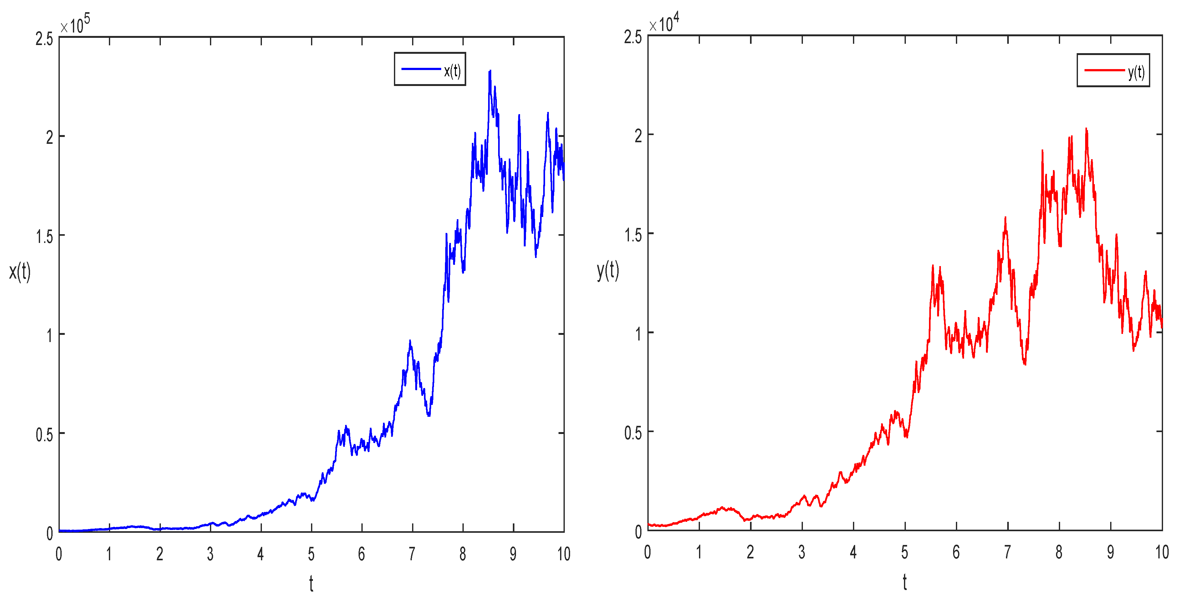
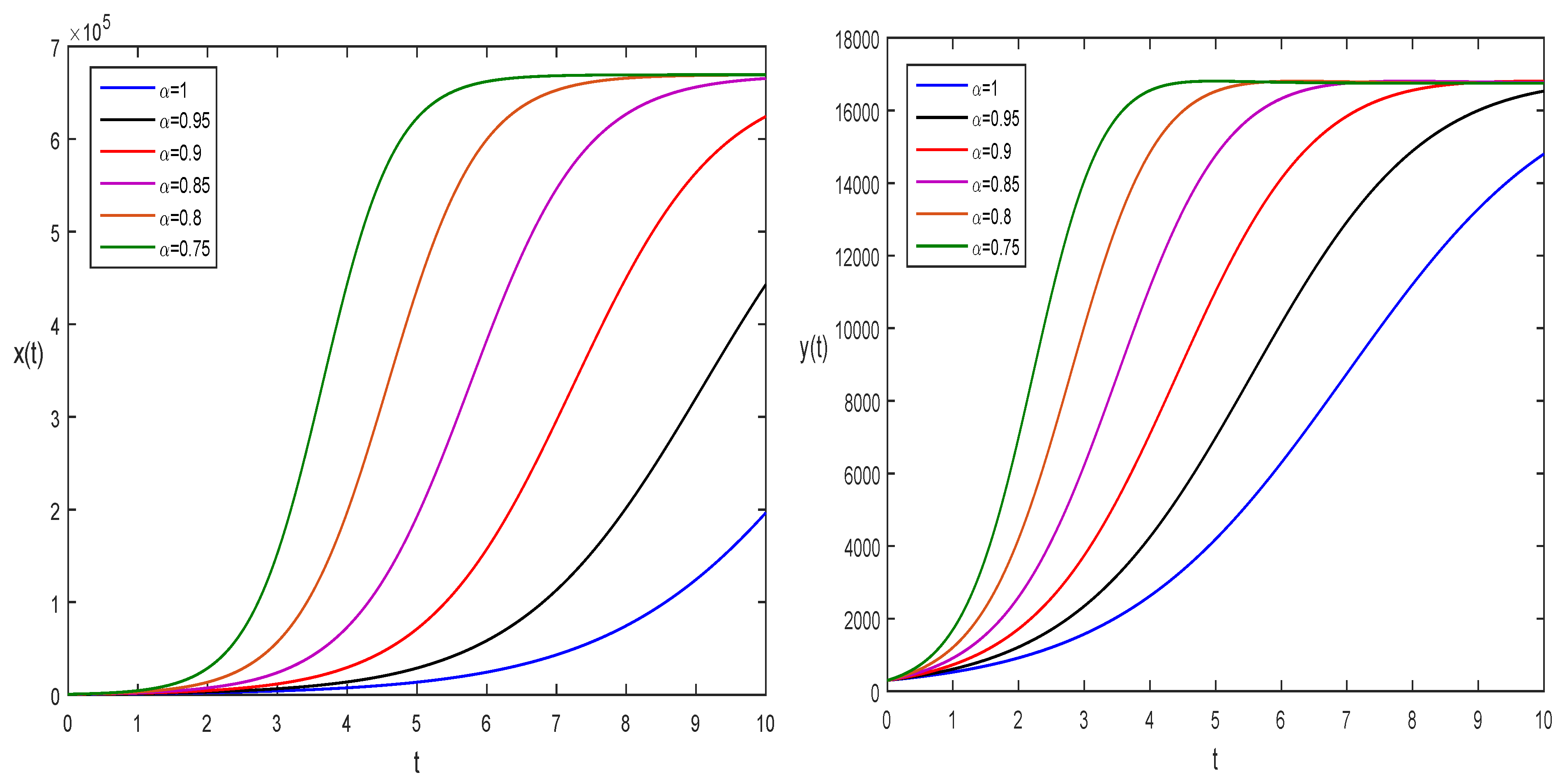
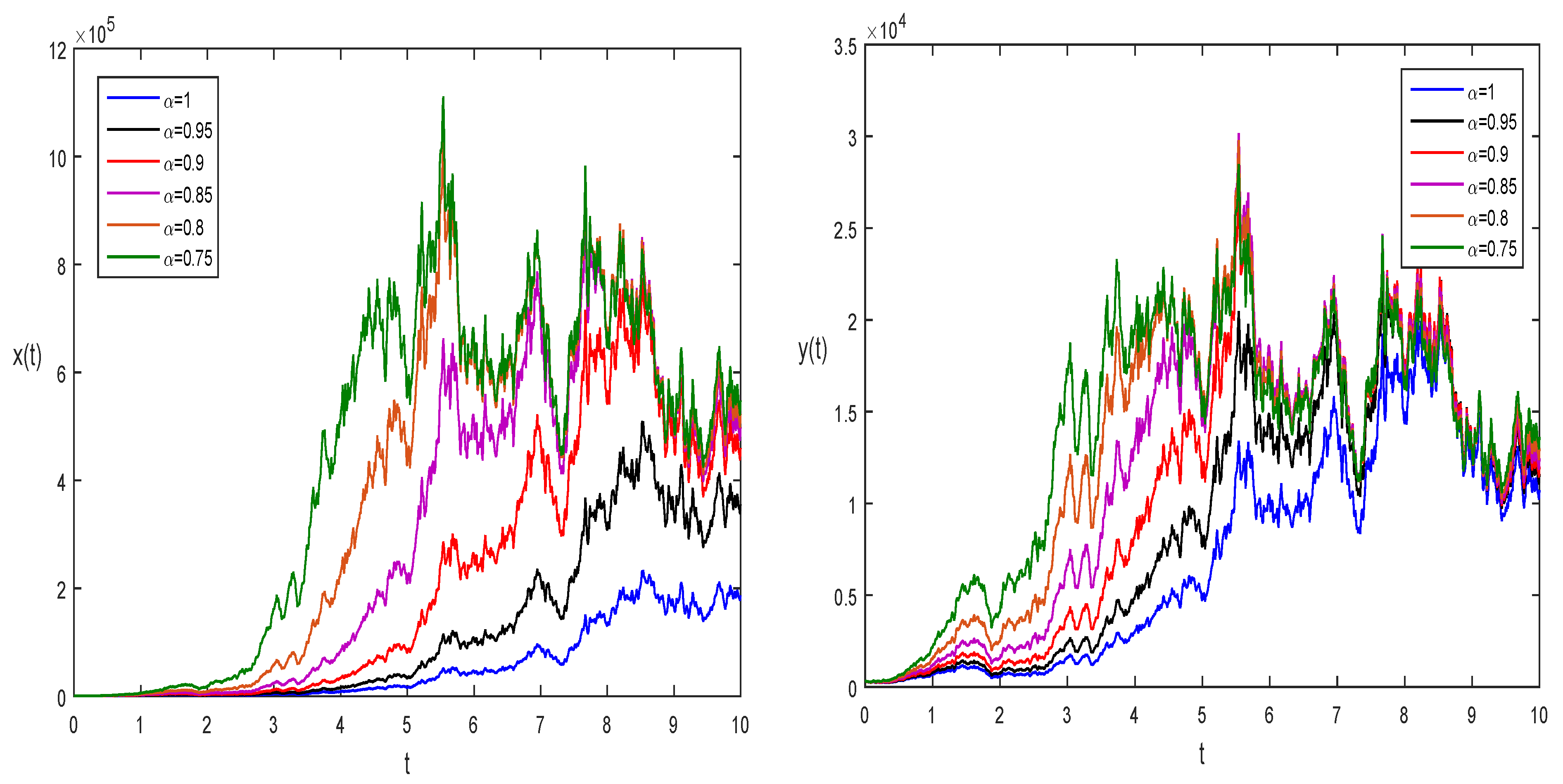
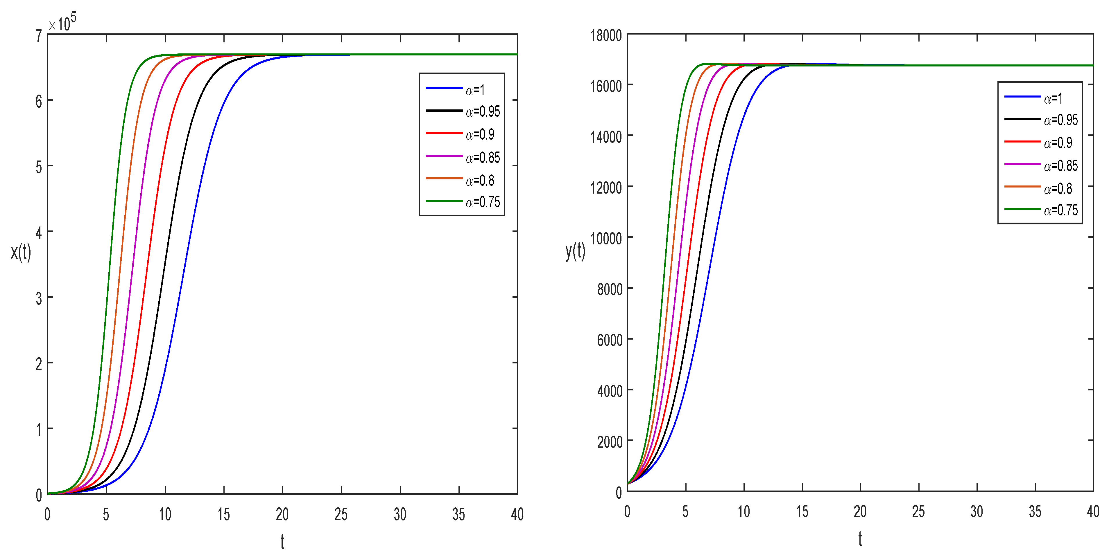
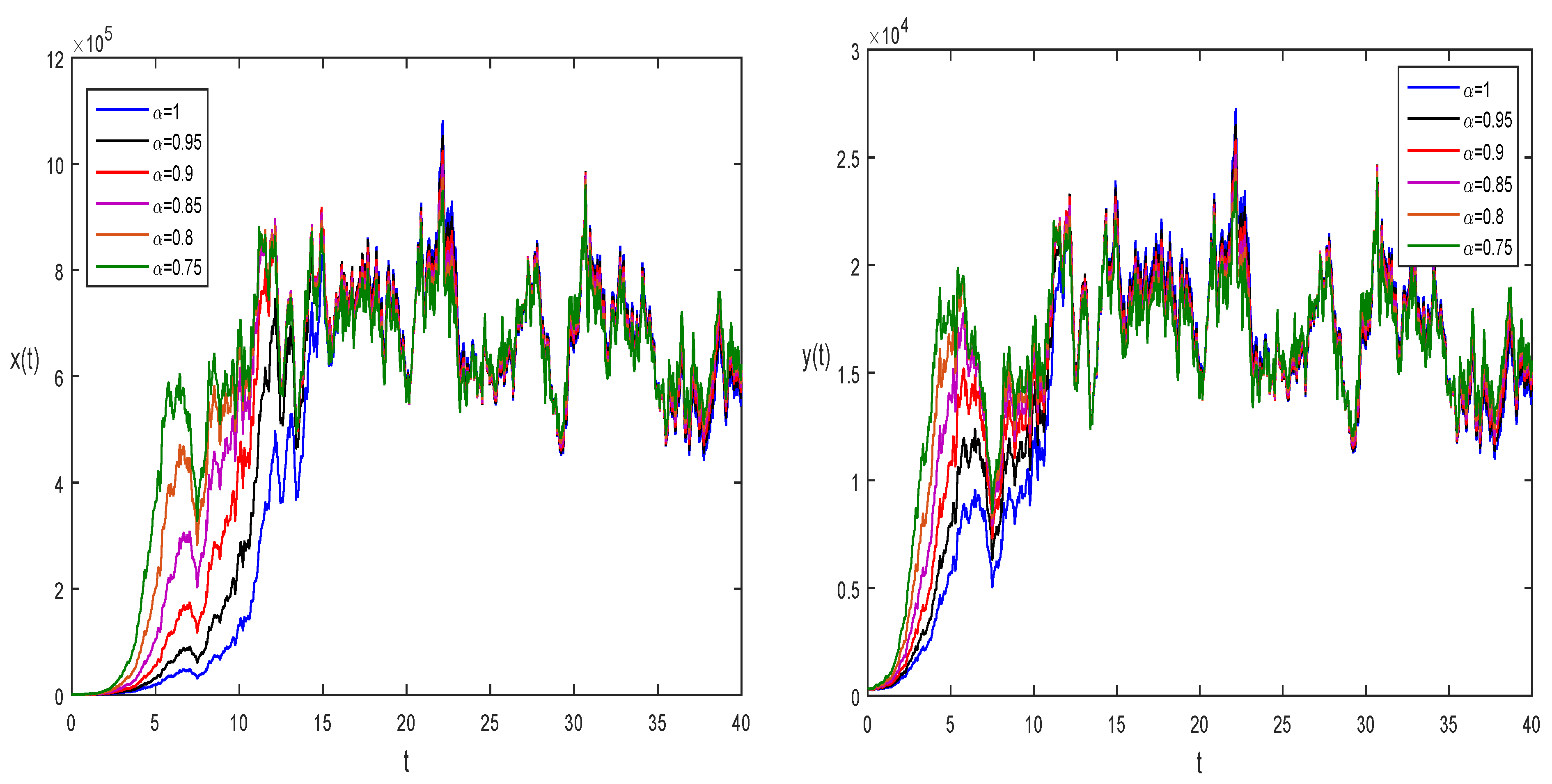
In this section, numerical simulations are performed for the fractional model in the AB derivative using the efficient numerical technique based on Legendre polynomials. Throughout this work, we evaluated the model parameters of the competition between the two banking systems using real statistical data [21]. The parameter values β 1 = 2.90 × 10 10 , β 2 = 3.90 × 10 8 ,   p 1 = 669,318 ,   p 2 = 17,540.6219 ,   r 1 = 0.6 , and r 2 = 0.58 were used in simulations. These parameter estimates are consistent with the the available results. Once those conditions were satisfied, the outcomes were shown in graphical form. Figure 1 displays the total number of responses from both urban and rural financial institutions, which are given in the deterministic system in Equation (1). Figure 2 demonstrates the goodness-of-fit of the stochastic model Equation (2) to the data for α = 1 . Figure 3 shows the comparison of fitting the real-world model given in Equations (1) and (2). Moreover, in Figure 4, we draw the deterministic system in Equation (1) to fictitious data with different fractional parameters α = 0.9 ; 0.8 ; 0.7 ; similarly, in Figure 5, we show the stochastic system in Equation (2) for the same parameter values. As can be seen in Figure 3 and Figure 4, decreasing the fractional order α might result in a better fit between the data and the model. Figure 5 shows the potential outcomes that might be anticipated with the use of real-world statistical data. A large body of evidence suggests that the model accurately represents the data over a wide range of time intervals. The findings are shown in Figure 6 by a large sample of integers and possess a unique solution given in Theorem 1. Figure 7 is drawn using a large random sample of integers which satisfy the statements of Theorems 1 and 2. Figure 5, Figure 6 and Figure 7 also indicate that when the proposed approach for Equation (29) is put into place, the system’s rural and commercial fractional models compete fiercely with one another with numerous fractional order parameters. All the simulations were performed using a personal desktop computer with an Intel(R) Core(TM) i5-2390T processor CPU at 2.70 GHz, 64-bit, and RAM of 4.00 GB.

5. Conclusions

In this work, we investigated a model based on real data to show how economic indicators shift over time using the fractional calculus approach. We created a numerical representation of the financial institution to use it as a basis for the proposed model using the integer order to include fractional operators such as Atangana–Baleanu. We used different parameter values of fractional order until we found the best match to represent the observed data. The fractional models were compared to the models of the integer order, which showed that the latter strategies are useful when it comes to data fitting in real situations. The divergence in the Atangana–Baleanu instance was made clear by the data fitting for the fractional case. It was shown that for the value of α equal to one or very close to one, the fractional operators and real-data comparison revealed some surprising similarities between the two of them. We also investigated the long-term tendencies of all three fractional operators and drew important conclusions over a wide range of values for the fractional order parameter α and showed that Atangana–Baleanu operator produces the better results because of its higher depth and breadth, as well as its appealing graphical features. Our numerical simulation shows that that the Atangana–Baleanu operator stands out above the others since it produces the highest quality results and can be used for the widest range of real-world problems.

Author Contributions

Conceptualization, I.A. and S.U.K.; methodology, I.A. and S.U.K.; software, S.U.K.; validation, I.A. and S.U.K.; formal analysis, I.A.; investigation, S.U.K.; resources, I.A.; writing—original draft preparation, I.A. and S.U.K.; writing—review and editing, I.A. and S.U.K.; supervision, I.A.; project administration, I.A.; funding acquisition, I.A. All authors have read and agreed to the published version of the manuscript.

Funding

This work was supported by the Deanship of Scientific Research, Vice Presidency for Graduate Studies and Scientific Research, King Faisal University, Saudi Arabia [GRANT No. 2727].

Data Availability Statement

Not applicable.

Acknowledgments

This work was supported by the Deanship of Scientific Research, Vice Presidency for Graduate Studies and Scientific Research, King Faisal University, Saudi Arabia [GRANT No. 2727].

Conflicts of Interest

The authors declare no conflict of interest.

References

  1. Hastings, A. (Ed.) Population Biology: Concepts and Models; Springer Science and Business Media: Berlin/Heidelberg, Germany, 2013. [Google Scholar]
  2. Ojk, Statistik Perbankan Indonesia 2004–2014. Available online: http://www.ojk.go.id/datastatistikperbankan-indonesia (accessed on 16 May 2015).
  3. Kim, J.; Lee, D.J.; Ahn, J. A dynamic competition analysis on the Korean mobile phone market using competitive diffusion model. Comput. Ind. Eng. 2006, 51, 174–182. [Google Scholar] [CrossRef]
  4. Michalakelis, C.; Christodoulos, C.; Varoutas, D.; Sphicopoulos, T. Dynamic estimation of markets exhibiting a preypredator behavior. Expert. Appl. 2012, 39, 7690–7700. [Google Scholar] [CrossRef]
  5. Lakka, S.; Michalakelis, C.; Varoutas, D.; Martakos, D. Competitive dynamics in the operating systems market: Modeling and policy implications. Technol Forecast Social Change. Comput. Math. Methods Med. 2013, 80, 88–105. [Google Scholar]
  6. Comes, C.A. Banking system: Three level Lotka-Volterra model. Procedia Econ. Financ. 2012, 3, 251–255. [Google Scholar] [CrossRef] [Green Version]
  7. Khan, M.A.; Azizah, M.; Ullah, S. A fractional model for the dynamics of competition between commercial and rural banks in Indonesia. Chaos Solitons Fractals 2019, 122, 32–46. [Google Scholar]
  8. Cai, G.Q.; Lin, Y.K. Stochastic analysis of the Lotka-Volterra model for ecosystems. Phys. Rev. E Stat. Nonlinear Soft Matter Phys. 2004, 70 Pt 1, 041910. [Google Scholar] [CrossRef]
  9. Ramanda, H.; Handari, B.D.; Aldila, D. Numerical simulation of stochastic model for deposit and loan volume based on the Lotka-Volterra model. Aip Conf. Proc. 2023, 2018, 020216. [Google Scholar]
  10. Arbi, S. Lembaga: Perbankan, Keuangan dan Pembiayaan; BPFE: Yogyakarta, Indonesia, 2013. [Google Scholar]
  11. Iskandar, S. Bank Dan Lembaga Keuangan Lainnya; Penerbit in Media: Jakarta, Indonesia, 2013. [Google Scholar]
  12. Owolabi, K.M.; Atangana, A. Mathematical analysis and computational experiments for an epidemic system with nonlocal and nonsingular derivative. Chaos Solitons Fractals 2019, 126, 41–49. [Google Scholar] [CrossRef]
  13. Atangana, A.; Khan, M.A. Validity of fractal derivative to capturing chaotic attractors. Chaos Solitons Fractals 2019, 126, 50–59. [Google Scholar] [CrossRef]
  14. Qureshi, S.; Atangana, A. Mathematical analysis of dengue fever outbreak by novel fractional operators with field data. Phys. A Stat. Mech. Its Appl. 2019, 526, 121127. [Google Scholar] [CrossRef]
  15. Mesgarani, H.; Rashidinia, J.; Aghdam, Y.E.; Nikan, O. Numerical treatment of the space fractional advection–dispersion model arising in groundwater hydrology. Comp. Appl. Math. 2021, 40, 22. [Google Scholar] [CrossRef]
  16. Oderinu, R.A.; Owolabi, J.A.; Taiwo, M. Approximate solutions of linear time-fractional differential equations. J. Math. Comput. Sci. 2023, 29, 60–72. [Google Scholar] [CrossRef]
  17. AlAhmad, R.; AlAhmad, Q.; Abdelhadi, A. Solution of fractional autonomous ordinary differential equations. J. Math. Comput. Sci. 2022, 27, 59–64. [Google Scholar] [CrossRef]
  18. Akram, T.; Abbas, M.; Ali, A. A numerical study on time fractional Fisher equation using an extended cubic B-spline approximation. J. Math. Comput. Sci. 2021, 22, 85–96. [Google Scholar] [CrossRef]
  19. Kilbas, A.A.; Srivastava, H.M.; Trujillo, J.J. Theory and Applications of Fractional Differential Equations, Volume 204 of North-Holland Mathematics Studies; Elsevier Science Inc.: New York, NY, USA, 2006. [Google Scholar]
  20. Podlubny, I. Fractional Differential Equations; Academic Press: New York, NY, USA, 1999. [Google Scholar]
  21. Wang, W.; Khan, M.A.; Fatmawati; Kumam, P.; Thounthong, P. A comparison study of bank data in fractional calculus. Chaos Solitons Fractals 2019, 126, 369–384. [Google Scholar] [CrossRef]
  22. Qureshi, S.; Yusuf, A. Fractional derivatives applied to MSEIR problems: Comparative study with real world data. Eur. J. Plus 2019, 134, 1–13. [Google Scholar] [CrossRef]
  23. Yusuf, A.; Qureshi, S.; Inc, M.; Aliyu, A.I.; Baleanu, D.; Shaikh, A.A. Two-strain epidemic model involving fractional derivative with Mittag-Leffler kernel. Chaos Interdiscip. Nonlinear Sci. 2018, 28, 123121. [Google Scholar] [CrossRef]
  24. Butt, A.I.K.; Imran, M.; Chamaleen, D.B.D.; Batool, S. Optimal control strategies for the reliable and competitive mathematical analysis of Covid-19 pandemic model. Math. Methods Appl. Sci. 2023, 46, 1528–1555. [Google Scholar] [CrossRef]
  25. Afzal, M.; Ismaeel, T.; Butt, A.I.K.; Farooq, Z.; Ahmad, R.; Khan, I. On the reducibility of a class of almost-periodic linear Hamiltonian systems and its application in Schr–dinger equation. AIMS Math. 2023, 8, 7471–7489. [Google Scholar] [CrossRef]
  26. Butt, A.I.K.; Ahmad, W.; Rafiq, M.; Baleanu, D. Numerical analysis of Atangana-Baleanu fractional model to understand the propagation of a novel corona virus pandemic. Alex. Eng. J. 2022, 61, 7007–7027. [Google Scholar] [CrossRef]
  27. Butt, A.I.K.; Imran, M.; Batool, S.; Nuwairan, M.A. Theoretical Analysis of a COVID-19 CF-Fractional Model to Optimally Control the Spread of Pandemic. Symmetry 2023, 15, 380. [Google Scholar] [CrossRef]
  28. Ali, A.; Khan, S.U.; Ali, I.; Khan, F.U. On dynamics of stochastic avian influenza model with asymptomatic carrier using spectral method. Math. Methods Appl. Sci. 2022, 45, 8230–8246. [Google Scholar] [CrossRef]
  29. Gul, N.; Khan, S.U.; Ali, I.; Khan, F.U. Transmission dynamic of stochastic hepatitis C model by spectral collocation method. Comput. Methods Biomech. Biomed. Eng. 2022, 25, 578–592. [Google Scholar] [CrossRef] [PubMed]
  30. Algehyne, E.A.; Khan, F.U.; Khan, S.U.; Jamshed, W.; Tag El Din, E.S.M. Dynamics of Stochastic Zika Virus with Treatment Class in Human Population via Spectral Method. Symmetry 2022, 14, 2137. [Google Scholar] [CrossRef]
  31. Khan, S.U.; Ali, I. Application of Legendre spectral-collocation method to delay differential and stochastic delay differential equation. AIP Adv. 2018, 8, 035301. [Google Scholar] [CrossRef] [Green Version]
  32. Khan, S.U.; Ali, I. Convergence and error analysis of a spectral collocation method for solving system of nonlinear Fredholm integral equations of second kind. Comput. Appl. Math. 2019, 38, 125. [Google Scholar] [CrossRef]
  33. Khan, S.U.; Ali, I. Applications of Legendre spectral collocation method for solving system of time delay differential equations. Adv. Mech. Eng. 2020, 12, 1–13. [Google Scholar] [CrossRef]
  34. Ali, I. Convergence analysis of spectral methods for integro-differential equations with vanishing proportional delays. J. Comput. Math. 2011, 29, 49–60. [Google Scholar] [CrossRef]
  35. Khan, S.U.; Ali, I. Numerical analysis of stochastic SIR model by Legendre spectral collocation method. Adv. Mech. Eng. 2019, 11, 1687814019862918. [Google Scholar] [CrossRef] [Green Version]
  36. Ali, I.; Khan, S.U. Analysis of stochastic delayed SIRS model with exponential birth and saturated incidence rate. Chaos Solitons Fractals 2020, 138, 110008. [Google Scholar] [CrossRef]
  37. Ali, I.; Khan, S.U. Threshold of stochastic SIRS epidemic model from infectious to susceptible class with saturated incidence rate using spectral method. Symmetry 2022, 14, 1838. [Google Scholar] [CrossRef]
  38. Ali, I.; Khan, S.U. Asymptotic Behavior of Three Connected Stochastic Delay Neoclassical Growth Systems Using Spectral Technique. Mathematics 2022, 10, 3639. [Google Scholar] [CrossRef]
  39. Ali, I.; Saleem, M.T. Applications of Orthogonal Polynomials in Simulations of Mass Transfer Diffusion Equation Arising in Food Engineering. Symmetry 2023, 15, 527. [Google Scholar] [CrossRef]
  40. Muhammad Altaf, K.; Atangana, A. Dynamics of Ebola Disease in the Framework of Different Fractional Derivatives. Entropy 2019, 21, 303. [Google Scholar] [CrossRef] [PubMed] [Green Version]
  41. Atangana, A.; Baleanu, D. New fractional derivatives with nonlocal and non-singular kernel: Theory and application to heat transfer model. Therm. Sci. 2016, 20, 763–769. [Google Scholar] [CrossRef] [Green Version]
  42. Zada, A.; Yar, M.; Li, T. Existence and stability analysis of nonlinear sequential coupled system of Caputo fractional differential equations with integral boundary conditions. Ann. Univ. Paedagog. Cracoviensis Stud. 2019, 17, 103–125. [Google Scholar] [CrossRef] [Green Version]
  43. Das, S.; Gupta, P.K. A mathematical model on fractional Lotka-Volterra equations. J. Theor. Biol. 2011, 277, 1–6. [Google Scholar] [CrossRef]
  44. Toufik, M.; Atangana, A. New numerical approximation of fractional derivative with non-local and non-singular kernel: Application to chaotic models. Eur. Phys. J. Plus 2017, 132, 444. [Google Scholar] [CrossRef]
  45. Morales-Delgado, V.F.; Gómez-Aguilar, J.F.; Saad, K.; Escobar Jiménez, R.F. Application of the Caputo-Fabrizio and Atangana-Baleanu fractional derivatives to mathematical model of cancer chemotherapy effect. Math. Methods Appl. Sci. 2019, 42, 1167–1193. [Google Scholar] [CrossRef]
  46. Owolabi, K.M. Numerical approach to fractional blow-up equations with Atangana-Baleanu derivative in Riemann-Liouville sense. Math. Model. Nat. Phenom. 2018, 13, 7. [Google Scholar] [CrossRef]
  47. Alb Lupaş, A.; Cătaş, A. Applications of the Atangana–Baleanu Fractional Integral Operator. Symmetry 2022, 14, 630. [Google Scholar] [CrossRef]
  48. Angstmann, C.N.; Jacobs, B.A.; Henry, B.I.; Xu, Z. Intrinsic Discontinuities in Solutions of Evolution Equations Involving Fractional Caputo–Fabrizio and Atangana–Baleanu Operators. Mathematics 2020, 8, 2023. [Google Scholar] [CrossRef]
  49. Sabatier, J.; Farges, C.; Tartaglione, V. Some Alternative Solutions to Fractional Models for Modelling Power Law Type Long Memory Behaviours. Mathematics 2020, 8, 196. [Google Scholar] [CrossRef] [Green Version]
  50. Baleanu, D.; Fernandez, A. On Fractional Operators and Their Classifications. Mathematics 2019, 7, 830. [Google Scholar] [CrossRef] [Green Version]
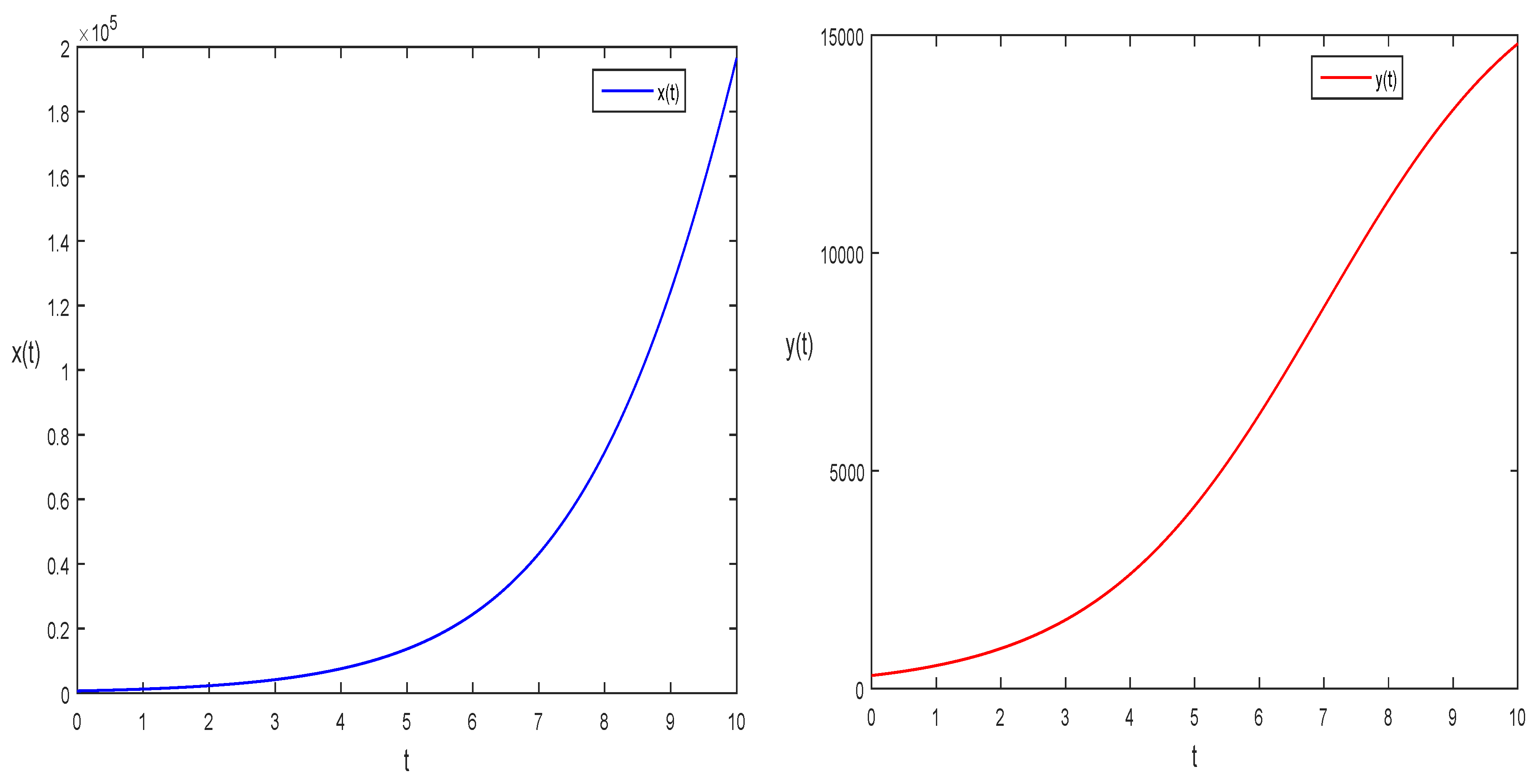
Figure 1. Solution behavior of system given in Equation (1).
Mathematics 11 01328 g001
Figure 2. Solution behavior of system given in Equation (2).
Mathematics 11 01328 g002
Figure 3. Comparison of the solutions of both the systems given in Equations (1) and (2).
Mathematics 11 01328 g003
Figure 4. Simulation of deterministic fractional model in Equation (14) for different fractional parameter values.
Mathematics 11 01328 g004
Figure 5. Simulations of fractional stochastic model in Equation (30) for different fractional parameter values.
Mathematics 11 01328 g005
Figure 6. Unique solution of deterministic fractional model in Equation (14) for different fractional parameter values.
Mathematics 11 01328 g006
Figure 7. Unique solution of fractional stochastic model in Equation (30) for different fractional parameter values.
Mathematics 11 01328 g007
Disclaimer/Publisher’s Note: The statements, opinions and data contained in all publications are solely those of the individual author(s) and contributor(s) and not of MDPI and/or the editor(s). MDPI and/or the editor(s) disclaim responsibility for any injury to people or property resulting from any ideas, methods, instructions or products referred to in the content.