Abstract
We use a quantile machine learning (random forests) approach to analyse the predictive ability of newspapers-based macroeconomic attention indexes (MAIs) on eight major fundamentals of the United States on the realized volatility of a major commodity-exporting emerging stock market, namely South Africa. We compare the performance of the MAIs with the performance of a news sentiment index (NSI) of the US. We find that both fundamentals and sentiment improve predictive performance, but the relative impact of the former is stronger. We document how the impact of fundamentals and sentiment on predictive performance varies across the quantiles of the conditional distribution of realized volatility, and across different prediction horizons. Specifically, fundamentals matter more at the extreme quantiles at short horizons, and at the median in the long-run. In addition, we report several robustness checks (involving sample period and alternative definitions of realized volatility), and indicate that the obtained results for South Africa also tend to carry over to other emerging countries such as, Brazil, China, India, and Russia. Our results have important implications for investors with volatility being an input for portfolio allocation decisions. In addition, with stock market variability also capturing financial uncertainty, its accurate prediction based on US fundamentals and sentiment also has a role in policy design to prevent possible collapse.
Keywords:
stock markets; realized volatility; macroeconomic attention; sentiment; quantile random forests; prediction models; BRICS countries MSC:
62-04; 62-07; 62-P05; 62-P20
JEL Classification:
C22; C53; E00; G15; G41
1. Introduction
Appropriate modelling and predicting of volatility is important due to several reasons, as outlined in [1]: Firstly, when volatility is interpreted as uncertainty, it becomes a key input to investment decisions and portfolio choices. Secondly, volatility is the most important variable in the pricing of derivative securities. To price an option, one needs reliable estimates of the volatility of the underlying assets. Thirdly, financial risk management according to the Basel Accord as established in 1996 also requires modelling and prediction of volatility as a compulsory input to risk management for financial institutions around the world. Finally, financial market volatility, as witnessed during the Global Financial Crisis and the COVID-19 pandemic, can have wide repercussions on the economy as a whole, via its effect on real economic activity and public confidence. Hence, estimates of market volatility can serve as a measure for the vulnerability of financial markets and the economy, and can help policy makers design appropriate policies. Evidently, appropriate modelling and accurate predictability of the process of volatility based on factors (predictors), has ample implications for portfolio selection, the pricing of derivative securities and risk management [2], making it a metric of paramount importance to not only investors, but also policy makers. Hence, not surprisingly the associated international academic literature on stock market volatility, in terms of econometric methods and predictors being considered, is massive to say the least, with a proper review being beyond the scope of this paper. We refer interested readers to the works of [3,4,5,6,7] for detailed discussions in this regard.
Against this backdrop of the importance of volatility modelling, and given the fact that macroeconomic news involving movements of fundamentals of the United States (US) have been found in earlier research to drive the volatility of the South African stock market [8], our aim in this paper is to revisit this issue in greater detail based on a sophisticated machine learning methodology (as will be discussed below). The finding of [8] is in line with the extant international literature in this regard (see, for example, [9,10,11,12,13]). Ref. [8] showed that surprises about inflation and unemployment rate announcements carried predictive content for the stock market volatility of the Johannesburg stock exchange (JSE), based on the Glosten–Jagannathan–Runkle-generalized autoregressive conditional heteroskedasticity (GJR-GARCH) model [14]. In addition, we also draw comparisons of our findings related to US fundamentals on the South African stock market volatility with the role of economic sentiment of the US, the influence of which on the South African stock returns variability has been reported by [15,16]. In other words, we aim to compare the influence of US fundamentals versus behavioural aspects in shaping the risk profile of the stock market of an emerging market economy. Although our focus is on South Africa mainly, we also contextualize our findings relative to other major emerging markets, namely Brazil, China, India and Russia. This contextualization helps us to provide a comprehensive understanding of the impact of the US-based fundamentals and sentiments on the entire BRICS bloc, which is now well-established as providing diversification benefits to international investors [17].
The choice of South Africa as the main component of our case study is driven not only by the availability of stock market data spanning over four decades in our analyses (1980 to 2020), but also because the need to conduct a focussed analysis of the South African stock market is warranted due to its sophistication. Moreover, South Africa is one of the largest exporters of highly financialized strategic commodities such as coal, chrome, diamond, gold, ilmenite, iron ore, manganese, palladium, platinum, rutile, vanadium, vermiculite, and zirconium [18]. Being a commodity-based economy, South Africa is globally well-integrated, and in light of the dominance of the US economy in the world financial system, changes in its macroeconomic fundamentals and behavioural components are likely to affect international financial markets in general and the South African stock market in particular, besides domestically, given that asset prices are functions of the state variables of the economy, shaped by the dynamics of fundamentals and sentiments [19,20]. At the same time, emerging markets are subjected to US investment flows, as a matter of portfolio diversification, hence, changes in the macroeconomic and behavioural environment of the US affects its domestic and global investment potential, which in turn is likely to feed into the risk status of the stock markets of emerging market economies [21,22]. The theoretical grounding of stock return volatility dates back to the [23], which states that stock return volatility is mainly caused by leverage effects, i.e., basically affected by news on fundamentals and/or sentiment. Naturally, in light of the connectivity of the global economy, theoretical models of volatility, should incorporate the information of not only domestic shocks, but also international innovation to macroeconomic and financial variables in the state-space of asset price variability. This is more so for emerging markets, which are susceptible to global surprises, while simultaneously acting as portfolio diversification outlets.
Specifically speaking, using a long-horizon prediction model, we evaluate the predictability of monthly stock market realized volatility of South Africa, and the BRIC countries, with newspaper-based macroeconomic attention indexes (MAIs) of the US on eight fundamentals (unemployment, monetary policy, output growth, inflation, housing market, credit ratings, oil, and the US dollar) with comparisons drawn with a newspaper-based measure of US economic sentiment. Realized volatility, as captured by the (log) square root of the sum of squared daily log-returns (following [24]), is considered as an accurate, observable, and unconditional metric of volatility [25], unlike the measures of the same derived from the popular alternative types of GARCH models, that has been primarily used in the South African stock market context to capture volatility (see for example, [26,27,28,29,30,31,32,33,34,35,36], and references cited therein), as well as the stochastic volatility (SV) framework. At this stage, it must be noted, within the GARCH-class of models, volatility analysis in South Africa has been dominated by univariate frameworks, and when multivariate-settings were indeed adopted to capture information of predictors, focus was primarily on domestic variables [37,38,39]. More importantly, we use quantile random forests [40], a flexible data-driven machine learning technique, to derive inferences from our prediction models. This machine learning technique is capable of capturing complex non-linear and interaction effects in a natural way from the fundamentals- and sentiment-based predictors mentioned above, which could be as many as seventeen in number in a full model. Moreover, quantile random forests allow the predictive value of the US MAIs and sentiment to be traced out along the quantiles of the conditional distribution of realized volatility. This is advantageous for a risk manager looking to invest in the BRICS, who could need information of whether movements in fundamentals or sentiment precede turbulent market phases, and hence may be not so much interested in a prediction of the conditional mean but rather some upper quantile of future realized volatility.
To the best of our knowledge, we are the first to compare the importance of MAIs versus sentiment of the US economy in predicting realized volatility of the stock returns of South Africa and the BRIC countries using a quantile-based machine learning technique. In a sense, our research can be considered an extension of the recent work by [41], who highlight the importance of the MAIs, particularly at longer horizons, in predicting the path of realized volatility of the G7 (Canada, France, Germany, Italy, Japan, the United Kingdom (UK), and the US) stock markets. Hence, our paper takes an emerging markets perspective, and goes beyond the conditional-mean-based predictive regression approach by considering quantile random forests to study the entire conditional distribution of the realized volatility of the BRICS, information of which should be of immense value to risk managers, given that these are economies known to provide portfolio diversification opportunities beyond developed equity markets. We organize the remainder of our research as follows: we describe our data in Section 2, while we lay out our empirical methods in Section 3. We discuss in Section 4 our empirical results, and finally we conclude in Section 5.
2. Data
We computed the square root of the sum of squared daily log-returns of the JSE stock index and, thus, considered the classical estimator of realized variance as per [24], with the underlying data derived from Refinitiv Datastream. In our predictive analyses, we used the square root of realized variance (that is, realized volatility, ) to scale down on the large spikes in the data during various periods of crises over the sample period, and we considered the natural logarithm of to bring the empirical distribution of realized volatility closer to a normal distribution. We shall also report, however, in Section 4 results for realized variance and the anti-log of realized volatility.
Reference [42] observed that market participants, in addition to the level of volatility, also care about the nature of volatility, with investors typically differentiating between “good” upside (calculated based on the sum of squared daily positive log-returns only) and “bad” downside (calculated based on the sum of squared daily negative log-returns only) volatilities. In light of this, we also predicted the logarithms of good and bad s, besides overall . We plot the along with good and bad in Figure 1.
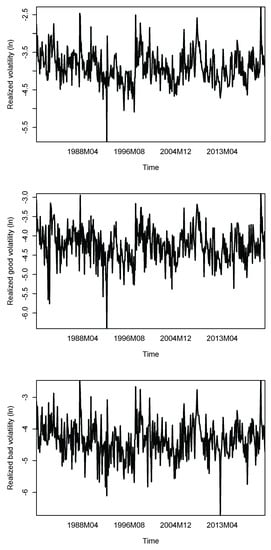
Figure 1.
Realized volatility.
As far as our predictors are concerned, the MAIs are indicators constructed by [43] to focus on different macroeconomic risks of the US. (The MAIs can be downloaded from the data segment of the internet page of Professor Jinfei Sheng at https://sites.google.com/site/shengjinfei/data?authuser=0, accesed on 31 January 2023) To this end, the authors consider eight macroeconomic news categories. These eight categories capture risks associated with unemployment, monetary policy, output growth, inflation, housing market, credit ratings, oil, and the US dollar. They then measure the attention of each category by building a word list to count the number of articles in every category. The MAIs are constructed based on a text corpus of articles from the New York Times (NYT) and the Wall Street Journal (WSJ).
In terms of our behavioural variable dealing with economic sentiment, we utilize the news sentiment index (NSI) developed by [44], which is based on a lexical analysis of economics-related news articles from 24 major US newspapers (compiled by the news aggregator service Factiva). (The data can be downloaded from: https://www.frbsf.org/economic-research/indicators-data/daily-news-sentiment-index/, accessed on 31 January 2023). The articles that the researchers selected were those with at least 200 words which Factiva identified as dealing with “economics” as the topic, and the “United States” as the subject country. Finally, they combined publicly available lexicons with their news-specific lexicon and constructed a sentiment-scoring model designed specifically for newspaper articles.
When using MAIs derived from the NYT with or without the NSI, our analyses covers June 1980 to December 2020, while the same is January 1984 to December 2020, when we rely on the WSJ-based MAIs (with or without the NSI), while the sentiment index data stretches back to January 1980.
3. Methods
A standard way to examine the link between realized volatility, fundamentals, and sentiment is to estimate a long-horizon prediction model of the following format:
where denotes an intercept term, and , and denote slope coefficients (or coefficient vectors) to be estimated, denotes a disturbance term, denotes the realized volatility, the parameter h denotes the prediction horizon, and (for ) denotes the average realized volatility over the relevant horizon. The term on the right-hand side of Equation (1) controls for the presence of autocorrelation of realized volatility, and the term denotes fundamentals or sentiment (or both).
The long-horizon prediction model formalized in Equation (1) sheds light on the effect of fundamentals and sentiment on the conditional mean of subsequent realized volatility and, thus, may be of limited use in certain situations when it comes to risk management. A risk manager, for example, who needs information of whether movements in fundamentals or sentiment precede turbulent market phases may not be so interested in a prediction of the conditional mean but rather at some upper quantile of subsequent realized volatility. A natural extension of the long-horizon prediction model, thus, is to estimate Equation (1) as a quantile-regression model (Koenker and Bassett, 1978; Koenker 2004) [45,46]. The quantile-regression version of the long-run prediction model is given by
where denotes the quantile being studied, denotes the quantile-dependent coefficient vector (a hat denotes an estimated parameter), and , denotes the check function, defined as if and if .
Estimation of the long-run prediction models given in Equations (1) and (2) is complicated when the number of predictors is large. In our empirical analysis, for example, we study various sources of fundamentals, and from two different newspapers. A large number of predictors naturally inflates the number of coefficients to be estimated. In addition, the various fundamentals and sentiment predictors are likely to interact, and accounting for such interactions may help to improve upon the predictive performance of the prediction models. In addition, the link between subsequent realized volatility and its predictors may be non-linear in some cases, such that it would be advantageous to have available a version of the long-run prediction model that accounts, preferably in a purely data-driven way, for predictor interactions and potential non-linearities in the data. A quantile-regression forest is such a model. A recent application of quantile-regression forests in empirical finance can be found in a paper by [47]. The following exposition of how a quantile-regression forest works closely draws on the discussion in that paper.
A quantile-regression forest consists of many individual regression trees. A regression tree, in turn, consists of a root, interior nodes, and terminal nodes (for a comprehensive textbook exposition, see [48]). The nodes recursively partition the space of predictors into subspaces (this partitioning is done in a top-down and binary way). The formation of such subspaces starts at the top level of a regression tree by choosing a partitioning predictor, s (that is, one of the right-hand side variables in Equations (1) and (2)), and a partitioning point, z, in such a way as to form two regions and , which are obtained as the solutions to the optimization problem , where , with , , denotes that the period t realization of predictor s belongs to region , and denotes the realizations of realized volatility in region k. Hence, the regions can be interpreted to represent areas of relative homogeneity of realized volatility. This region-formation process then proceeds in a recursive and hierarchical way until every leaf contains a minimum number of observations of realized volatility or some maximal tree size is reached (a researcher defines these “hyperparameters” in advance).
An individual regression tree clearly represents a complex hierarchical object, and this object highly depends on the data on which it is grown. A complex individual regression tree, thereby, is likely to have poor predictive ability when it is applied to new data. A random forest overcomes this problem of individual regression trees in three ways. First, a random forest is a forest and as such consists of many individual trees. Second, the individual trees that make up a random forest are random regression trees. A random regression tree differs from a standard regression tree in that it is grown by choosing a random subset of the predictors in every step of the region-formation process. Third, every single random regression tree that is a member of a random forest is estimated on a bootstrapped sample of the data [49]. Averaging predictions across many random regression trees stabilizes predictions, where choosing a random subset of the predictors mitigates the influence of individual influential predictors, and bootstrapping the data decorrelates the predictions from individual random regression trees.
Importantly, bootstrapping the data has the further advantage that a random forest can easily by used to compute predictions of realized volatility based on the hold-out (or, in the terminology of the machine learning literature, the out-of-bag) data. In our empirical research, we use these out-of-bag predictions to study the predictive value of fundamentals and sentiment for subsequent realized volatility. Studying out-of-bag predictions has the advantage that a random forest (or, in our case, a quantile random forest) is grown by sampling from the full sample of data. Hence, studying the predictive value of fundamentals and sentiment by means of the out-of-bag predictions use information from the entire sample. At the same time, the out-of-bag predictions, unlike conventional predictions obtained from exploiting the information in the full sample of data, are not merely in-sample predictions, but they can be interpreted as quasi “out-of-sample” predictions obtained by averaging the predictions of random regression trees on hold-out (“test”) data. In a sense, the out-of-bag predictions can be interpreted to blend elements of in-sample and pure out-of-sample testing, while the latter is often considered as an ultimate test of predictive ability, the former may have a higher power and, therefore, may be more credible than the latter [50].
Building on the research on random forests, Ref. [40] developed quantile random forests. Intuitively, the basic idea is that a quantile random forest stores not only information on the mean of realized volatility at the leaves (as a conventional regression tree does) but rather keeps all observations of realized volatility, and then uses this information to compute an estimate, , of the conditional distribution function of realized volatility. The -quantile of the conditional distribution function is defined such that the probability that realized volatility is smaller than , given , is equal to , with an estimate of the -quantile being computed as .
We used the R language and environment for statistical computing [51] to carry out our empirical research, where we used the R add-on package “grf” [52] to estimate the quantile-random-forest versions of our long-horizon prediction models (using the “quantregForest” developed by [53] gave qualitatively similar results; not reported for reasons of space), where we used 2000 trees to form a random forest, and largely used default values for the other hyperparameters.
We estimated various versions of our long-run prediction models: models that feature only autoregressive terms, models that feature only fundamentals/sentiment as predictors, models with feature both fundamentals and sentiment as predictors, and models that rely on only WSJ fundamentals or only NYT fundamentals as predictors. We used these different versions of our long-run prediction models to trace out the contribution of fundamentals versus sentiment to the predictive performance of the models. To this end, we plugged the out-of-bag predictions of realized volatility implied by the various long-run prediction models into a relative performance statistic (see also [54,55]). The relative performance, , statistic accounts for the performance, given the quantile being analysed, and is given by
where again denotes the check function, denotes the prediction error implied by a benchmark model, and denotes the prediction error implied by a rival model. Equation (3) makes clear that, given a quantile, the rival model performs better than the benchmark model when , while the benchmark model dominates the rival model when . It should be noted that, we evaluated out-of-bag predictions under the loss (check) function. Hence, the relative performance statistic is a metric of the relative predictive value of the benchmark and the rival model at the quantile being studied in terms of a loss-function-weighted sum of absolute prediction errors [54]. It follows that the relative performance statistic is a quantile-specific, local measure of relative predictive performance rather than a global measure evaluated over the entire conditional distribution of realized volatility [55].
4. Empirical Results
We summarize the results for the relative performance statistic for our baseline scenario in Table 1 for five different quantiles, , and four different prediction horizons, . We computed the relative performance statistic based on the out-of-bag predictions of the quantile-random-forest long-run prediction models. Panel A summarizes results for the NYT fundamentals, while panel B depicts the results for the WSJ fundamentals. In the baseline scenario, we use a simple first-order autoregressive model as our benchmark model. A positive relative performance statistic indicates that the rival model, given in the first column of the table, outperforms the benchmark model. The relative performance statistic is positive throughout all model specifications, quantiles, and prediction horizons (with only one minor exception). The message to take home, thus, is that the fundamental-/sentiment-based models outperform the benchmark model, where this effect is stronger for the fundamental-based model than for the sentiment-based models. Hence, fundamentals tend to matter more for the out-of-bag predictive performance than sentiment. We also observe, for both fundamentals and sentiment, that the relative performance statistic increases in the prediction horizon for the quantiles beyond the median. When the model features fundamentals as predictors, its relative performance also improves when we study the median. It should be noted that the MAIs and the NSI are also available at a daily frequency. Given this, following the extant literature on the South African stock market, we first obtained daily estimates of conditional volatility using GARCH models over the period from 1 June 1980 to 31 December 2020, and 1 January 1984 to 31 December 2020 to correspond to the MAIs derived from the NYT and WSJ. Complete details of the parameter estimates of the GARCH model are available upon request from the authors. Then, in the next step, we conducted a quantile-based bivariate causality test as outlined in [56], with the results reported in Table A1 at the end of the paper (Appendix A). The results are consistent with our results based on , different (standardized) fundamentals tend to consistently produce higher predictability (shown by higher values of the standard normal test statistic) compared to the (standardized) NSI for all the considered quantiles of 0.05, 0.25, 0.5, 0.75, and 0.95 for the WSJ data, and barring the quantile of 0.05 when we use the NYT-based MAIs.

Table 1.
AR model is the benchmark.
In Table 2, we report the results of a direct comparison between the models of that feature, on the one hand, fundamentals and, on the other hand, sentiment (in addition to an autoregressive term). (In Table A2, at the end of the paper, we report results of an analysis when the sample period starts in 1994, as that is when democratic South Africa came into being, with various international restrictions deregulated. The general picture that emerges from the results for the shorter sample period is the same as conveyed by the results in Table A2.) The negative relative performance statistic for the comparison of the fundamentals with the sentiment model shows that the predictive ability of the former clearly dominates that of the latter, where this result grows stronger for the long prediction horizons. This does not mean, however, that sentiment does not carry any predictive value. In fact, we observe a mainly positive relative performance statistic when we compare the fundamentals model with the fundamentals-come-sentiment model, while the positive relative performance statistic is smaller in absolute terms than when we compare the fundamentals model with the sentiment model, the results show that sentiment adds some incremental performance relative to fundamentals alone, which likely reflects that the QRF model captures interaction effects between both types of predictors. Not surprisingly, the fundamentals-come-sentiment model also performs better than the sentiment model, where the margin by which the fundamentals-come-sentiment model outperforms the sentiment model is larger than that we observe when we compare the fundamentals-cum-sentiment model with the fundamentals model. It is also interesting to observe that, when we compare fundamentals with sentiment, the relative performance statistic exhibits a U-shaped pattern across the quantiles for the short predictive horizons, which turns into an inverted U-shaped pattern for the long predictive horizons. Hence, fundamentals contribute more to relative predictive model performance at the upper and lower quantiles when one focuses on the short predictive horizons, while their relative contribution centres at the median for the long predictive horizon.
Table 2.
Sentiment vs. news.
The results we report in Table A3, Table A4 and Table A5 at the end of the paper (Appendix A) demonstrate that our baseline results carry over to “good” and “bad” realized volatility, and to a model that features ten autoregressive lags of realized volatility in the array of predictors. We computed good realized volatility based on data for days with positive returns, while bad realized volatility represents days with negative returns. Fundamentals add value to out-of-bag predictions in case of good realized volatility, where the direct comparison of the fundamental- and sentiment-based models shows that this effect is stronger for the long prediction horizon and the quantiles below the median. Moreover, the contribution to relative performance is stronger for the WSJ fundamentals than for the NYT fundamentals. For bad realized volatility, in turn, fundamentals have a large effect on out-of-bag predictive performance. Similarly, the WSJ fundamentals work better than the NYT fundamentals in the case of bad realized volatility and when we consider an the extended autoregressive benchmark model, especially so for the upper quantiles.
In Table 3, we compare the predictive ability of the NYT with that of the WSJ fundamentals, where we control for the effects of lagged realized volatility and sentiment. The results show that the WSJ fundamentals have a stronger predictive ability over subsequent realized volatility than the NYT fundamentals, an effect that grows stronger in the predictive horizon and for the quantiles below the median. Similarly, the model that features both types of fundamentals performs better than the model that only features the NYT fundamentals. Nonetheless, NYT fundamentals also have some incremental predictive value, as the results for a comparison of the model that features both types of fundamentals in its array of predictors with the model that only features the WSJ fundamentals demonstrates.
Table 3.
The role played by fundamentals: NYT fundamentals vs. WSJ fundamentals.
In Table 4, we report the results of two robustness checks. Specifically, we report results for realized volatility (that is, we do not study its natural logarithm) and squared realized volatility, that is, realized variance. The robustness checks, which are based on the WSJ fundamentals, corroborate our main result. Fundamentals have a stronger predictive value than sentiment, especially when we consider the longer predictive horizons (interestingly, this effect is strongest at the upper quantiles), but adding sentiment to the array of predictors further improves the incremental predictive value of the model on out-of-bag data.
Table 4.
Results for the anti-log of realized volatility and realized variance (WSJ fundamentals).
While our main results are based on out-of-bag predictions, we summarize some out-of-sample results in Table A6 at the end of the paper. In order to keep the analysis simple, we split the sample into an in-sample and and out-of-sample part. We then estimated the models on the in-sample part of the data, and used the out-of-sample part to make predictions of realized volatility. We used the last 15, 20, and 25% of the data for the out-of-sample part. The results show that the NYT fundamentals outperform sentiment when we use 20 or 25% of the data for the out-of-sample analysis. The results for an out-of-sample proportion of 15% are mixed. The results for the WSJ fundamentals are mixed as well. The WSJ fundamentals perform best relative to sentiment at the short predictive horizon. Importantly, the negative relative performance statistic reveals that, when we study the WSJ data (and to a lesser extent also for the NYT data), fundamentals dominate sentiment at the upper 95% quantiles of realized volatility, that is, our results imply that investors should take into account fundamentals when trying to compute upper tails (peaks) of realized volatility.
A reader also may wonder whether the results we obtained for South Africa are representative for the other BRIC countries, with the underlying daily data for the stock markets also derived from Refinitiv Datastream. The results for Brazil, China, India, and Russia, that we report in Table 5, show that this is indeed the case over the periods of July 1994–December 2020, August 1991–December 2020, January 1990–December 2020, and January 1998–December 2020. For estimation of the BRIC models, we used the WSJ fundamentals, but the results for the NYT fundamentals were qualitatively similar (see Table A7 at the end of the paper), while the details differ across the BRIC countries, we observe, as in the case of South Africa, that fundamentals have a stronger out-of-bag predictive value than sentiment, and that the contribution of fundamentals to relative out-of-bag predictive performance of the model being studied increases in the predictive horizon. Moreover, the relative out-of-bag predictive performance of a model that features both fundamentals and sentiment tends to be stronger when we compare such a comprehensive model with a model that features only sentiment than when we use a model that features fundamentals as our benchmark model.
Table 5.
Results for other BRIC countries (WSJ fundamentals).
Overall, we find that:
- While both fundamentals and sentiment have predictive value the relative impact of the former is stronger than that of the latter;
- The importance of accounting for fundamentals and sentiment varies across the quantiles of the conditional distribution of realized volatility, which motivates the quantiles-based approach we have used in our research;
- The importance of accounting for fundamentals and sentiment also varies across different prediction horizons that we have studied, where fundamentals are more important at the extreme quantiles when we consider short horizons, and at the median when we study the long-run horizon;
- Robustness checks corroborate our main findings. Importantly, our results for South Africa tend to carry over to the BRIC countries (Brazil, China, India, and Russia).
Having summarized our main findings, some comparisons can be drawn with a couple of related studies, namely) [8] and [41], though it must be realized that one-to-one correspondence is impossible with ours being the first paper to predict realized volatility of South Africa and the BRICS countries using quantile-based machine learning methods, applied to wide array of newspaper-derived predictors involving fundamentals and sentiments associated with the US economy. In general, we can conclude that, just like in [8], we can highlight the importance of US news on fundamentals, beyond unemployment and inflation, in defining the path of South African stock market volatility. These authors, however, rely on a GARCH model, and are not able to study the entire conditional distribution of realized volatility, as we do using quantile random forest, while we find that fundamentals matter more than sentiment in predicting the realized volatility of the BRICs stock markets, we also highlight the importance of the combined role of these predictors. This finding is actually in line with [41], who highlighted that combined information from economic policy uncertainty (EPU) with MAIs tends to perform better in terms of predicting stock market realized volatility of advanced economies, i.e., the G7, compared to models with just the fundamentals. It should be noted that the similarity arises when one recognizes that sentiment and uncertainty are strongly negatively correlated. In other words, for the predictability of risk involving both developed and emerging stock markets, news on macroeconomic variables and behavioural decisions contain complementary information. However, then again, unlike [41], who used conditional mean-based predictive regressions, our results are state-specific, and hence can be regarded as being more informative when dealing with realized volatility of the South Africa and the BRIC countries.
5. Concluding Remarks
Given that significant early research has established the importance of macroeconomic news of the US on international stock market volatility, we utilize quantile random forests, a machine learning technique, to predict the realized volatility of the South African stock market—one of the world’s major commodity exporters. In this regard, we use newspaper-based fundamentals and sentiments associated with the US economic performance, while some evidence exist on the role of US fundamentals in driving South African stock market volatility using GARCH models, we go beyond this research by considering information on a wider array of fundamentals, as well as sentiment, via the usage of a more robust, unconditional and observable measure of volatility, i.e., realized volatility, and utilizing a sophisticated quantile-based machine learning approach (random forest) to draw inferences. The econometric framework is capable of capturing complex non-linear and interaction effects in a natural way from the predictors, while simultaneously tracing out their predictive value along the quantiles of the conditional distribution of realized volatility, which corresponds to alternative states (levels). While the focus is on South Africa, we also compare our results with Brazil, China, India and Russia, i.e., the entire BRICS bloc. In the process, we make the first attempt to compare the importance of US fundamentals versus sentiment in predicting realized volatility of stock returns of the BRICS using a quantile-based machine learning technique. In this regard, we build on a similar investigation performed for the G7 countries, but which is limited to a conditional-mean-based predictive model.
The results of our empirical research shed light on how the impact of fundamentals and sentiment on predictive performance varies across the quantiles of the conditional distribution of realized volatility, and across different prediction horizons. A major finding is that, while both fundamentals and sentiment improve predictive performance, the relative impact of fundamentals outweighs that of sentiment. More specifically, fundamentals matter more at the extreme quantiles at short predictive horizons, and at the median in the long-run. Our results are robust to sample periods and alternative definitions of realized volatility. Finally, results for the BRIC countries corroborate the major empirical observations of South Africa.
Clearly, our findings are of obvious importance for investors looking for portfolio diversification involving investments in emerging stock markets. In particular, the information contained in US fundamentals can be used relatively efficiently compared to sentiment in accurately predicting realized volatility of emerging markets, while serving as a key input to investment decisions and portfolio choices. However, results are contingent on the state of the market, with the extremes/tails predictable in the short-run, and the median (normal) state in the long-horizon. At the same time, with stock market volatility also often interpreted as a measure of financial uncertainty, its predictability, based on the information contained in US fundamentals, should assist the South African policy authorities to design appropriate monetary and fiscal policy responses to prevent possible future recessions, especially if the future path of stock market volatility is expected to rise and produce a theoretically consistent reduction in economic activity [57].
As part of future research, contingent on the availability of newspaper-based macroeconomic attention and sentiment indexes for South Africa, it would be interesting to compare the role of such domestic predictors with those of the US considered in this paper, though it is likely that the latter will contain leading information for the former. Furthermore, in light of the recent emphasis on climate finance [58], one could also compare US news on uncertainty surrounding climate risks with the fundamentals and behavioural predictors. Some preliminary evidence in this regard, using the WSJ-reliant metric of climate risks of [59] (WSJ_Engle) over January 1984–June 2017; and the multiple newspaper-based climate policy uncertainty (CPU) index [60] for the period of April 1987–August 2022, the environmental policy (EnvP) index (as well as two sub-topic indexes for renewable energy policy (EnvP_REP) and international climate negotiations (EnvP_ICN)) over January 1981–March 2019, and environmental policy uncertainty (EnvPU) index covering October 1990–March 2019 (with the last four indexes developed by [61]), depicting evidence of predictability over the conditional distribution of the South African stock market , as derived from the causality-in-quantiles test of [56]. The evidence of in-sample prediction from these indexes of the US is particularly strong around the median, as can be observed from Table A8 in the Appendix A. Furthermore, when compared between good and bad realized volatilities, the test statistic is generally higher under the latter, indicative of the negative impact of climate risks on conventional stock returns.
At this stage, it is important to point out a possible limitation of our work, while newspaper-based indexes dealing with fundamental-related information have the advantages of being possibly exogenous, and are also able to measure otherwise latent variables, such as sentiments, news on these topics can itself be biased due to the possibility of the media being managed. Having said this, the chances of such concerns emanating from our reliable news sources are less likely, but reliance on actual values of fundamentals especially may be a viable route to undertake, though this is often involved with publication lags, low-frequency, and endogeneity concerns.
Author Contributions
Conceptualization, R.G.; methodology, J.N. and C.P.; software, C.P.; validation, R.G. and C.P.; formal analysis, J.N. and C.P.; investigation, R.G., J.N. and C.P.; resources, R.G., J.N. and C.P.; data curation, R.G. and J.N.; writing—original draft preparation, R.G. and C.P.; writing—review and editing, R.G., J.N. and C.P.; visualization, R.G., J.N. and C.P.; project administration, R.G. All authors have read and agreed to published version of manuscript.
Funding
This research received no external funding.
Data Availability Statement
Data will be made available upon request.
Conflicts of Interest
The authors declare no conflict of interest.
Appendix A

Figure A1.
New York Times fundamentals.
Figure A1.
New York Times fundamentals.


Figure A2.
Wall Street Journal fundamentals.
Figure A2.
Wall Street Journal fundamentals.


Figure A3.
Sentiment.
Figure A3.
Sentiment.

Table A1.
Causality-in-quantiles results for daily GARCH-based volatility estimates of South Africa: fundamentals versus sentiment.
Table A1.
Causality-in-quantiles results for daily GARCH-based volatility estimates of South Africa: fundamentals versus sentiment.
| Panel A: New York Times | |||||
|---|---|---|---|---|---|
| Quantiles | 0.05 | 0.25 | 0.5 | 0.75 | 0.95 |
| Credit Ratings | 2.937 *** | 6.652 *** | 4.784 *** | 3.32 *** | 1.363 |
| GDP | 2.702 *** | 5.988 *** | 4.886 *** | 3.573 *** | 1.641 |
| Housing Market | 3.519 *** | 6.337 *** | 4.57 *** | 3.27 *** | 1.297 |
| Inflation | 3.352 *** | 7.243 *** | 6.094 *** | 4.247 *** | 1.862 * |
| Monetary Policy | 2.457 ** | 6.334 *** | 5.363 *** | 4.734 *** | 1.859 * |
| Oil Price | 3.097 *** | 7.117 *** | 5.445 *** | 3.382 *** | 1.475 |
| Unemployment | 2.665 *** | 5.961 *** | 5.115 *** | 4.217 *** | 1.51 |
| US Dollar | 3.622 *** | 8.17 *** | 5.332 *** | 2.92 *** | 1.116 |
| NSI | 4.105 *** | 6.348 *** | 5.151 *** | 4.676 *** | 1.723 * |
| Panel B: Wall Street Journal | |||||
| Quantiles | 0.05 | 0.25 | 0.5 | 0.75 | 0.95 |
| Credit Ratings | 3.111 *** | 5.683 *** | 5.159 *** | 5.178 *** | 1.729 * |
| GDP | 2.739 *** | 7.215 *** | 5.797 *** | 4.468 *** | 2.13 ** |
| Housing Market | 2.992 *** | 6.388 *** | 5.365 *** | 4.166 *** | 1.906 * |
| Inflation | 2.846 *** | 6.301 *** | 5.465 *** | 4.889 *** | 2.024 ** |
| Monetary Policy | 3.082 *** | 6.831 *** | 5.984 *** | 4.49 *** | 2.038 ** |
| Oil Price | 3.07 *** | 6.105 *** | 5.415 *** | 4.527 *** | 1.861 * |
| Unemployment | 2.698 *** | 6.944 *** | 5.804 *** | 4.624 *** | 2.165 ** |
| US Dollar | 3.218 *** | 6.171 *** | 5.057 *** | 4.545 *** | 2.025 ** |
| NSI | 2.996 *** | 6.316 *** | 5.71 *** | 4.792 *** | 2.117 ** |
***, **, and * indicate rejection of the null hypothesis of no causality at the 1, 5, and 10% level of significance at a quantile based on the standard normal test statistic of Jeong et al. (2012) [56]. Credit ratings, GDP, housing market, inflation, monetary policy, oil price, unemployment, and US dollar are the daily macroeconomic attention indexes (MAIs) of Fisher et al. (2022) [43]. NSI: news sentiment index of Shapiro et al. (2020) [44]. The bold entries depict the highest value of the statistic for a specific quantile across the predictors.
Table A2.
Sentiment vs. news (sample starts in 1994).
Table A2.
Sentiment vs. news (sample starts in 1994).
| Panel A: New York Times | ||||
|---|---|---|---|---|
| Benchmark/Rival Model | h = 1 | h = 3 | h = 6 | h = 12 |
| AR-fundamentals vs. AR-sentiment/q = 0.05 | −0.0469 | 0.0557 | −0.1138 | −0.1266 |
| AR-fundamentals vs. AR-sentiment/q = 0.25 | −0.0111 | −0.0459 | −0.1565 | −0.2992 |
| AR-fundamentals vs. AR-sentiment/q = 0.5 | −0.0346 | −0.1118 | −0.2152 | −0.3691 |
| AR-fundamentals vs. AR-sentiment/q = 0.75 | −0.0388 | −0.0907 | −0.3819 | −0.4759 |
| AR-fundamentals vs. AR-sentiment/q = 0.95 | −0.0591 | −0.1450 | −0.2885 | −0.1635 |
| AR-fundamentals vs. AR-fundamentals-sentiment/q = 0.05 | 0.0133 | 0.0258 | 0.0123 | −0.0004 |
| AR-fundamentals vs. AR-fundamentals-sentiment/q = 0.25 | 0.0040 | 0.0325 | 0.0232 | 0.0136 |
| AR-fundamentals vs. AR-fundamentals-sentiment/q = 0.5 | 0.0084 | 0.0096 | 0.0004 | 0.0139 |
| AR-fundamentals vs. AR-fundamentals-sentiment/q = 0.75 | 0.0133 | −0.0022 | −0.0003 | 0.0241 |
| AR-fundamentals vs. AR-fundamentals-sentiment/q = 0.95 | −0.0299 | 0.0125 | 0.0104 | 0.0528 |
| AR-sentiment vs. AR-fundamentals-sentiment/q = 0.05 | 0.0575 | −0.0317 | 0.1132 | 0.1120 |
| AR-sentiment vs. AR-fundamentals-sentiment/q = 0.25 | 0.0149 | 0.0750 | 0.1554 | 0.2407 |
| AR-sentiment vs. AR-fundamentals-sentiment/q = 0.5 | 0.0416 | 0.1092 | 0.1774 | 0.2797 |
| AR-sentiment vs. AR-fundamentals-sentiment/q = 0.75 | 0.0501 | 0.0812 | 0.2761 | 0.3388 |
| AR-sentiment vs. AR-fundamentals-sentiment/q = 0.95 | 0.0277 | 0.1375 | 0.2320 | 0.1859 |
| Panel B: Wall Street Journal | ||||
| Benchmark/rival model | h = 1 | h = 3 | h = 6 | h = 12 |
| AR-fundamentals vs. AR-sentiment/q = 0.05 | −0.0936 | 0.0294 | −0.1502 | −0.1982 |
| AR-fundamentals vs. AR-sentiment/q = 0.25 | −0.0287 | −0.0874 | −0.1804 | −0.3568 |
| AR-fundamentals vs. AR-sentiment/q = 0.5 | −0.0316 | −0.0985 | −0.1765 | −0.4303 |
| AR-fundamentals vs. AR-sentiment/q = 0.75 | −0.0512 | −0.0733 | −0.2656 | −0.5416 |
| AR-fundamentals vs. AR-sentiment/q = 0.95 | −0.0490 | −0.1603 | −0.3040 | −0.3689 |
| AR-fundamentals vs. AR-fundamentals-sentiment/q = 0.05 | 0.0270 | 0.0341 | 0.0038 | −0.0157 |
| AR-fundamentals vs. AR-fundamentals-sentiment/q = 0.25 | −0.0074 | 0.0394 | 0.0285 | 0.0104 |
| AR-fundamentals vs. AR-fundamentals-sentiment/q = 0.5 | 0.0011 | 0.0222 | 0.0221 | 0.0122 |
| AR-fundamentals vs. AR-fundamentals-sentiment/q = 0.75 | 0.0119 | 0.0257 | 0.0219 | 0.0163 |
| AR-fundamentals vs. AR-fundamentals-sentiment/q = 0.95 | −0.0082 | −0.0075 | 0.0587 | 0.0203 |
| AR-sentiment vs. AR-fundamentals-sentiment/q = 0.05 | 0.1103 | 0.0049 | 0.1339 | 0.1524 |
| AR-sentiment vs. AR-fundamentals-sentiment/q = 0.25 | 0.0207 | 0.1166 | 0.1770 | 0.2706 |
| AR-sentiment vs. AR-fundamentals-sentiment/q = 0.5 | 0.0317 | 0.1099 | 0.1688 | 0.3094 |
| AR-sentiment vs. AR-fundamentals-sentiment/q = 0.75 | 0.0600 | 0.0923 | 0.2272 | 0.3619 |
| AR-sentiment vs. AR-fundamentals-sentiment/q = 0.95 | 0.0389 | 0.1317 | 0.2782 | 0.2843 |
The relative performance statistic, RP, is computed as , where et denotes the model prediction errors. The benchmark (B) model is the first model given in the first column of the table, and the rival (R) model is the second model given in that column. Both models are estimated by means of quantile random forests and the relative performance statistic is computed based on the out-of-bag data. A positive RP statistic shows that the rival model outperforms the benchmark model. The parameter h denotes the forecast horizon. The parameter q denotes the quantile being analysed. The dependent variable is the natural log of the realized volatility.
Table A3.
Results for good realized volatility.
Table A3.
Results for good realized volatility.
| Panel A: New York Times | ||||
|---|---|---|---|---|
| Benchmark/Rival Model | h = 1 | h = 3 | h = 6 | h = 12 |
| AR-fundamentals vs. AR-sentiment/q = 0.05 | −0.1140 | −0.0785 | −0.3312 | −0.3936 |
| AR-fundamentals vs. AR-sentiment/q = 0.25 | −0.0540 | −0.1097 | −0.1975 | −0.3026 |
| AR-fundamentals vs. AR-sentiment/q = 0.5 | −0.0601 | −0.1105 | −0.2153 | −0.3721 |
| AR-fundamentals vs. AR-sentiment/q = 0.75 | −0.0772 | −0.1491 | −0.2623 | −0.4423 |
| AR-fundamentals vs. AR-sentiment/q = 0.95 | −0.0672 | −0.0498 | −0.1890 | −0.2185 |
| AR-fundamentals vs. AR-fundamentals-sentiment/q = 0.05 | −0.0084 | −0.0038 | 0.0056 | 0.0097 |
| AR-fundamentals vs. AR-fundamentals-sentiment/q = 0.25 | −0.0097 | 0.0165 | 0.0132 | 0.0108 |
| AR-fundamentals vs. AR-fundamentals-sentiment/q = 0.5 | 0.0043 | 0.0085 | 0.0070 | 0.0325 |
| AR-fundamentals vs. AR-fundamentals-sentiment/q = 0.75 | 0.0035 | 0.0135 | 0.0229 | 0.0775 |
| AR-fundamentals vs. AR-fundamentals-sentiment/q = 0.95 | 0.0108 | 0.0209 | 0.0282 | 0.1030 |
| AR-sentiment vs. AR-fundamentals-sentiment/q = 0.05 | 0.0948 | 0.0692 | 0.2530 | 0.2894 |
| AR-sentiment vs. AR-fundamentals-sentiment/q = 0.25 | 0.0421 | 0.1137 | 0.1759 | 0.2407 |
| AR-sentiment vs. AR-fundamentals-sentiment/q = 0.5 | 0.0607 | 0.1071 | 0.1829 | 0.2949 |
| AR-sentiment vs. AR-fundamentals-sentiment/q = 0.75 | 0.0749 | 0.1415 | 0.2259 | 0.3604 |
| AR-sentiment vs. AR-fundamentals-sentiment/q = 0.95 | 0.0731 | 0.0673 | 0.1827 | 0.2638 |
| Panel B: Wall Street Journal | ||||
| Benchmark/rival model | h = 1 | h = 3 | h = 6 | h = 12 |
| AR-fundamentals vs. AR-sentiment/q = 0.05 | −0.0685 | −0.1259 | −0.5055 | −0.6304 |
| AR-fundamentals vs. AR-sentiment/q = 0.25 | −0.0637 | −0.1979 | −0.2556 | −0.4922 |
| AR-fundamentals vs. AR-sentiment/q = 0.5 | −0.0787 | −0.1928 | −0.2967 | −0.5269 |
| AR-fundamentals vs. AR-sentiment/q = 0.75 | −0.1073 | −0.1486 | −0.3748 | −0.5887 |
| AR-fundamentals vs. AR-sentiment/q = 0.95 | −0.1513 | −0.1811 | −0.4067 | −0.5345 |
| AR-fundamentals vs. AR-fundamentals-sentiment/q = 0.05 | 0.0153 | 0.0216 | 0.0395 | −0.0111 |
| AR-fundamentals vs. AR-fundamentals-sentiment/q = 0.25 | 0.0136 | 0.0137 | 0.0306 | 0.0356 |
| AR-fundamentals vs. AR-fundamentals-sentiment/q = 0.5 | 0.0048 | 0.0153 | 0.0357 | 0.0164 |
| AR-fundamentals vs. AR-fundamentals-sentiment/q = 0.75 | −0.0011 | 0.0273 | 0.0115 | 0.0438 |
| AR-fundamentals vs. AR-fundamentals-sentiment/q = 0.95 | −0.0177 | 0.0055 | 0.0099 | 0.0495 |
| AR-sentiment vs. AR-fundamentals-sentiment/q = 0.05 | 0.0785 | 0.1310 | 0.3620 | 0.3799 |
| AR-sentiment vs. AR-fundamentals-sentiment/q = 0.25 | 0.0726 | 0.1767 | 0.2279 | 0.3537 |
| AR-sentiment vs. AR-fundamentals-sentiment/q = 0.5 | 0.0774 | 0.1744 | 0.2563 | 0.3558 |
| AR-sentiment vs. AR-fundamentals-sentiment/q = 0.75 | 0.0959 | 0.1532 | 0.2810 | 0.3981 |
| AR-sentiment vs. AR-fundamentals-sentiment/q = 0.95 | 0.1161 | 0.1580 | 0.2962 | 0.3806 |
The relative performance statistic, RP, is computed as , where et denotes the model prediction errors. The benchmark (B) model is the first model given in the first column of the table, and the rival (R) model is the second model given in that column. Both models are estimated by means of quantile random forests and the relative performance statistic is computed based on the out-of-bag data. A positive RP statistic shows that the rival model outperforms the benchmark model. The parameter h denotes the forecast horizon. The parameter q denotes the quantile being analysed. The dependent variable is the natural log of the realized volatility.
Table A4.
Results for bad realized volatility.
Table A4.
Results for bad realized volatility.
| Panel A: New York Times | ||||
|---|---|---|---|---|
| Benchmark/Rival Model | h = 1 | h = 3 | h = 6 | h = 12 |
| AR-fundamentals vs. AR-sentiment/q = 0.05 | −0.1077 | −0.0851 | −0.1286 | −0.2268 |
| AR-fundamentals vs. AR-sentiment/q = 0.25 | −0.0478 | −0.0689 | −0.1088 | −0.2600 |
| AR-fundamentals vs. AR-sentiment/q = 0.5 | −0.0419 | −0.0440 | −0.1418 | −0.2885 |
| AR-fundamentals vs. AR-sentiment/q = 0.75 | −0.0340 | −0.0070 | −0.1687 | −0.2495 |
| AR-fundamentals vs. AR-sentiment/q = 0.95 | −0.0968 | −0.0087 | −0.2772 | −0.4335 |
| AR-fundamentals vs. AR-fundamentals-sentiment/q = 0.05 | −0.0033 | 0.0768 | 0.0147 | 0.0101 |
| AR-fundamentals vs. AR-fundamentals-sentiment/q = 0.25 | 0.0072 | 0.0154 | 0.0477 | 0.0160 |
| AR-fundamentals vs. AR-fundamentals-sentiment/q = 0.5 | 0.0086 | 0.0364 | 0.0511 | 0.0526 |
| AR-fundamentals vs. AR-fundamentals-sentiment/q = 0.75 | 0.0098 | 0.0390 | 0.0519 | 0.0645 |
| AR-fundamentals vs. AR-fundamentals-sentiment/q = 0.95 | −0.0457 | 0.0260 | 0.0560 | 0.0542 |
| AR-sentiment vs. AR-fundamentals-sentiment/q = 0.05 | 0.0943 | 0.1492 | 0.1270 | 0.1931 |
| AR-sentiment vs. AR-fundamentals-sentiment/q = 0.25 | 0.0525 | 0.0789 | 0.1412 | 0.2190 |
| AR-sentiment vs. AR-fundamentals-sentiment/q = 0.5 | 0.0485 | 0.0770 | 0.1689 | 0.2647 |
| AR-sentiment vs. AR-fundamentals-sentiment/q = 0.75 | 0.0424 | 0.0457 | 0.1887 | 0.2513 |
| AR-sentiment vs. AR-fundamentals-sentiment/q = 0.95 | 0.0466 | 0.0344 | 0.2609 | 0.3402 |
| Panel B: Wall Street Journal | ||||
| Benchmark/rival model | h = 1 | h = 3 | h = 6 | h = 12 |
| AR-fundamentals vs. AR-sentiment/q = 0.05 | −0.1692 | −0.2331 | −0.2211 | −0.4358 |
| AR-fundamentals vs. AR-sentiment/q = 0.25 | −0.0673 | −0.1081 | −0.2135 | −0.3168 |
| AR-fundamentals vs. AR-sentiment/q = 0.5 | −0.0634 | −0.0688 | −0.2261 | −0.4210 |
| AR-fundamentals vs. AR-sentiment/q = 0.75 | −0.0465 | −0.0700 | −0.2649 | −0.4625 |
| AR-fundamentals vs. AR-sentiment/q = 0.95 | −0.0124 | −0.0135 | −0.3831 | −0.7039 |
| AR-fundamentals vs. AR-fundamentals-sentiment/q = 0.05 | 0.0240 | 0.0283 | 0.0182 | 0.0040 |
| AR-fundamentals vs. AR-fundamentals-sentiment/q = 0.25 | −0.0034 | 0.0312 | 0.0304 | 0.0324 |
| AR-fundamentals vs. AR-fundamentals-sentiment/q = 0.5 | 0.0042 | 0.0201 | 0.0186 | 0.0173 |
| AR-fundamentals vs. AR-fundamentals-sentiment/q = 0.75 | 0.0045 | 0.0297 | 0.0005 | 0.0221 |
| AR-fundamentals vs. AR-fundamentals-sentiment/q = 0.95 | −0.0001 | 0.0133 | 0.0010 | 0.0184 |
| AR-sentiment vs. AR-fundamentals-sentiment/q = 0.05 | 0.1653 | 0.2120 | 0.1960 | 0.3063 |
| AR-sentiment vs. AR-fundamentals-sentiment/q = 0.25 | 0.0598 | 0.1257 | 0.2009 | 0.2652 |
| AR-sentiment vs. AR-fundamentals-sentiment/q = 0.5 | 0.0636 | 0.0832 | 0.1995 | 0.3085 |
| AR-sentiment vs. AR-fundamentals-sentiment/q = 0.75 | 0.0488 | 0.0932 | 0.2098 | 0.3313 |
| AR-sentiment vs. AR-fundamentals-sentiment/q = 0.95 | 0.0121 | 0.0264 | 0.2777 | 0.4239 |
The relative performance statistic, RP, is computed as , where et denotes the model prediction errors. The benchmark (B) model is the first model given in the first column of the table, and the rival (R) model is the second model given in that column. Both models are estimated by means of quantile random forests and the relative performance statistic is computed based on the out-of-bag data. A positive RP statistic shows that the rival model outperforms the benchmark model. The parameter h denotes the forecast horizon. The parameter q denotes the quantile being analysed. The dependent variable is the natural log of the realized volatility.
Table A5.
Results for AR(10) models.
Table A5.
Results for AR(10) models.
| Panel A: New York Times | ||||
|---|---|---|---|---|
| Benchmark/Rival Model | h = 1 | h = 3 | h = 6 | h = 12 |
| AR-fundamentals vs. AR-sentiment/q = 0.05 | −0.0096 | −0.0340 | −0.0041 | −0.0257 |
| AR-fundamentals vs. AR-sentiment/q = 0.25 | −0.0190 | −0.0441 | −0.0659 | −0.1787 |
| AR-fundamentals vs. AR-sentiment/q = 0.5 | −0.0283 | −0.0373 | −0.0757 | −0.2469 |
| AR-fundamentals vs. AR-sentiment/q = 0.75 | 0.0015 | −0.0281 | −0.1301 | −0.2221 |
| AR-fundamentals vs. AR-sentiment/q = 0.95 | −0.0316 | −0.0065 | −0.1136 | −0.1629 |
| AR-fundamentals vs. AR-fundamentals-sentiment/q = 0.05 | 0.0073 | 0.0036 | 0.0045 | 0.0259 |
| AR-fundamentals vs. AR-fundamentals-sentiment/q = 0.25 | −0.0026 | 0.0018 | 0.0116 | 0.0190 |
| AR-fundamentals vs. AR-fundamentals-sentiment/q = 0.5 | 0.0007 | 0.0105 | 0.0282 | 0.0432 |
| AR-fundamentals vs. AR-fundamentals-sentiment/q = 0.75 | 0.0038 | 0.0049 | 0.0212 | 0.0865 |
| AR-fundamentals vs. AR-fundamentals-sentiment/q = 0.95 | −0.0067 | 0.0045 | 0.0606 | 0.0796 |
| AR-sentiment vs. AR-fundamentals-sentiment/q = 0.05 | 0.0168 | 0.0363 | 0.0086 | 0.0502 |
| AR-sentiment vs. AR-fundamentals-sentiment/q = 0.25 | 0.0161 | 0.0440 | 0.0727 | 0.1677 |
| AR-sentiment vs. AR-fundamentals-sentiment/q = 0.5 | 0.0282 | 0.0461 | 0.0966 | 0.2326 |
| AR-sentiment vs. AR-fundamentals-sentiment/q = 0.75 | 0.0023 | 0.0322 | 0.1339 | 0.2525 |
| AR-sentiment vs. AR-fundamentals-sentiment/q = 0.95 | 0.0241 | 0.0109 | 0.1564 | 0.2085 |
| Panel B: Wall Street Journal | ||||
| Benchmark/rival model | h = 1 | h = 3 | h = 6 | h = 12 |
| AR-fundamentals vs. AR-sentiment/q = 0.05 | −0.0542 | −0.0373 | −0.0523 | −0.0843 |
| AR-fundamentals vs. AR-sentiment/q = 0.25 | −0.0048 | −0.0520 | −0.1013 | −0.2232 |
| AR-fundamentals vs. AR-sentiment/q = 0.5 | −0.0163 | −0.0332 | −0.1345 | −0.3867 |
| AR-fundamentals vs. AR-sentiment/q = 0.75 | −0.0060 | −0.0449 | −0.1460 | −0.3871 |
| AR-fundamentals vs. AR-sentiment/q = 0.95 | −0.0375 | −0.0883 | −0.2175 | −0.4157 |
| AR-fundamentals vs. AR-fundamentals-sentiment/q = 0.05 | −0.0090 | 0.0033 | 0.0157 | 0.0048 |
| AR-fundamentals vs. AR-fundamentals-sentiment/q = 0.25 | 0.0057 | 0.0225 | 0.0262 | 0.0312 |
| AR-fundamentals vs. AR-fundamentals-sentiment/q = 0.5 | 0.0045 | 0.0145 | 0.0147 | 0.0121 |
| AR-fundamentals vs. AR-fundamentals-sentiment/q = 0.75 | −0.0020 | 0.0190 | 0.0061 | 0.0302 |
| AR-fundamentals vs. AR-fundamentals-sentiment/q = 0.95 | 0.0038 | −0.0110 | −0.0029 | −0.0001 |
| AR-sentiment vs. AR-fundamentals-sentiment/q = 0.05 | 0.0428 | 0.0391 | 0.0646 | 0.0822 |
| AR-sentiment vs. AR-fundamentals-sentiment/q = 0.25 | 0.0105 | 0.0708 | 0.1158 | 0.2080 |
| AR-sentiment vs. AR-fundamentals-sentiment/q = 0.5 | 0.0205 | 0.0462 | 0.1315 | 0.2875 |
| AR-sentiment vs. AR-fundamentals-sentiment/q = 0.75 | 0.0039 | 0.0612 | 0.1328 | 0.3009 |
| AR-sentiment vs. AR-fundamentals-sentiment/q = 0.95 | 0.0398 | 0.0710 | 0.1763 | 0.2936 |
The AR part of the model comprises ten lags of RV. The relative performance statistic, RP, is computed as , where et denotes the model prediction errors. The benchmark (B) model is the first model given in the first column of the table, and the rival (R) model is the second model given in that column. Both models are estimated by means of quantile random forests and the relative performance statistic is computed based on the out-of-bag data. A positive RP statistic shows that the rival model outperforms the benchmark model. The parameter h denotes the forecast horizon. The parameter q denotes the quantile being analysed. The dependent variable is the natural log of the realized volatility.
Table A6.
Out-of-sample results.
Table A6.
Out-of-sample results.
| Panel A: New York Times | ||||
|---|---|---|---|---|
| Benchmark/Rival Model | h = 1 | h = 3 | h = 6 | h = 12 |
| Out-of-sample: 25% | ||||
| AR-fundamentals vs. AR-sentiment/q = 0.05 | 0.1537 | 0.0159 | −0.1712 | −0.1915 |
| AR-fundamentals vs. AR-sentiment/q = 0.25 | −0.1338 | −0.0425 | −0.0128 | −0.1417 |
| AR-fundamentals vs. AR-sentiment/q = 0.5 | −0.0958 | 0.0066 | −0.0424 | −0.2430 |
| AR-fundamentals vs. AR-sentiment/q = 0.75 | −0.0607 | −0.0070 | −0.0874 | −0.1890 |
| AR-fundamentals vs. AR-sentiment/q = 0.95 | −0.0343 | −0.1998 | −0.0423 | −0.0672 |
| Out-of-sample: 20% | ||||
| AR-fundamentals vs. AR-sentiment/q = 0.05 | −0.1252 | 0.0757 | −0.0882 | −0.1840 |
| AR-fundamentals vs. AR-sentiment/q = 0.25 | −0.0801 | −0.0506 | −0.0838 | −0.1546 |
| AR-fundamentals vs. AR-sentiment/q = 0.5 | −0.0921 | −0.0124 | −0.0898 | −0.2192 |
| AR-fundamentals vs. AR-sentiment/q = 0.75 | −0.0705 | 0.0002 | −0.1123 | −0.1946 |
| AR-fundamentals vs. AR-sentiment/q = 0.95 | −0.0508 | −0.2559 | −0.1231 | −0.1680 |
| Out-of-sample: 15% | ||||
| AR-fundamentals vs. AR-sentiment/q = 0.05 | −0.0190 | 0.0485 | 0.0145 | 0.0028 |
| AR-fundamentals vs. AR-sentiment/q = 0.25 | −0.0576 | −0.0058 | 0.0219 | −0.0465 |
| AR-fundamentals vs. AR-sentiment/q = 0.5 | −0.0060 | 0.0529 | 0.0048 | −0.0397 |
| AR-fundamentals vs. AR-sentiment/q = 0.75 | 0.0047 | 0.0357 | −0.0575 | −0.0516 |
| AR-fundamentals vs. AR-sentiment/q = 0.95 | 0.0429 | −0.3176 | −0.0861 | 0.0205 |
| Panel B: Wall Street Journal | ||||
| Benchmark/rival model | h = 1 | h = 3 | h = 6 | h = 12 |
| Out-of-sample: 25% | ||||
| AR-fundamentals vs. AR-sentiment/q = 0.05 | −0.0739 | 0.0664 | 0.0085 | 0.2426 |
| AR-fundamentals vs. AR-sentiment/q = 0.25 | −0.0901 | 0.0648 | 0.0180 | 0.0892 |
| AR-fundamentals vs. AR-sentiment/q = 0.5 | −0.0295 | 0.0672 | 0.0099 | −0.0585 |
| AR-fundamentals vs. AR-sentiment/q = 0.75 | −0.0643 | 0.0363 | −0.0181 | −0.2527 |
| AR-fundamentals vs. AR-sentiment/q = 0.95 | −0.1912 | −0.1784 | −0.1206 | −0.2116 |
| Out-of-sample: 20% | ||||
| AR-fundamentals vs. AR-sentiment/q = 0.05 | −0.1840 | 0.1358 | 0.0280 | 0.0111 |
| AR-fundamentals vs. AR-sentiment/q = 0.25 | −0.0281 | −0.0327 | 0.0474 | −0.0666 |
| AR-fundamentals vs. AR-sentiment/q = 0.5 | −0.0544 | 0.0513 | −0.0016 | −0.1274 |
| AR-fundamentals vs. AR-sentiment/q = 0.75 | −0.0983 | 0.0231 | −0.0193 | −0.4104 |
| AR-fundamentals vs. AR-sentiment/q = 0.95 | −0.2417 | −0.2303 | −0.1169 | −0.1446 |
| Out-of-sample: 15% | ||||
| AR-fundamentals vs. AR-sentiment/q = 0.05 | −0.0122 | 0.1282 | −0.0407 | 0.0532 |
| AR-fundamentals vs. AR-sentiment/q = 0.25 | 0.0341 | 0.0422 | 0.0700 | 0.0034 |
| AR-fundamentals vs. AR-sentiment/q = 0.5 | 0.0467 | 0.0643 | −0.0162 | −0.1406 |
| AR-fundamentals vs. AR-sentiment/q = 0.75 | −0.1059 | −0.0248 | −0.0714 | −0.3727 |
| AR-fundamentals vs. AR-sentiment/q = 0.95 | −0.0744 | −0.2748 | −0.1721 | −0.2604 |
The AR part of the model comprises ten lags of RV. The relative performance statistic, RP, is computed as , where et denotes the model prediction errors. The benchmark (B) model is the first model given in the first column of the table, and the rival (R) model is the second model given in that column. Both models are estimated by means of quantile random forests and the relative performance statistic is computed based on the out-of-bag data. A positive RP statistic shows that the rival model outperforms the benchmark model. The parameter h denotes the forecast horizon. The parameter q denotes the quantile being analysed. The dependent variable is the natural log of the realized volatility.
Table A7.
Results for other BRIC countries (NYT fundamentals).
Table A7.
Results for other BRIC countries (NYT fundamentals).
| Panel A: Brazil | ||||
|---|---|---|---|---|
| Benchmark/Rival Model | h = 1 | h = 3 | h = 6 | h = 12 |
| AR-fundamentals vs. AR-sentiment/q = 0.05 | −0.1428 | −0.1246 | −0.1103 | −0.3304 |
| AR-fundamentals vs. AR-sentiment/q = 0.25 | −0.0192 | −0.0824 | −0.1432 | −0.2976 |
| AR-fundamentals vs. AR-sentiment/q = 0.5 | −0.0301 | −0.0999 | −0.2164 | −0.3089 |
| AR-fundamentals vs. AR-sentiment/q = 0.75 | −0.0186 | −0.1658 | −0.2776 | −0.4311 |
| AR-fundamentals vs. AR-sentiment/q = 0.95 | −0.1091 | −0.2308 | −0.3533 | −0.6252 |
| AR-fundamentals vs. AR-fundamentals-sentiment/q = 0.05 | −0.0120 | 0.0272 | 0.0521 | 0.0011 |
| AR-fundamentals vs. AR-fundamentals-sentiment/q = 0.25 | 0.0038 | 0.0004 | 0.0177 | 0.0186 |
| AR-fundamentals vs. AR-fundamentals-sentiment/q = 0.5 | 0.0004 | 0.0088 | 0.0135 | 0.0046 |
| AR-fundamentals vs. AR-fundamentals-sentiment/q = 0.75 | −0.0026 | 0.0049 | 0.0089 | 0.0183 |
| AR-fundamentals vs. AR-fundamentals-sentiment/q = 0.95 | −0.0144 | 0.0064 | 0.0186 | 0.0328 |
| AR-sentiment vs. AR-fundamentals-sentiment/q = 0.05 | 0.1144 | 0.1351 | 0.1463 | 0.2492 |
| AR-sentiment vs. AR-fundamentals-sentiment/q = 0.25 | 0.0226 | 0.0765 | 0.1407 | 0.2437 |
| AR-sentiment vs. AR-fundamentals-sentiment/q = 0.5 | 0.0296 | 0.0988 | 0.1890 | 0.2395 |
| AR-sentiment vs. AR-fundamentals-sentiment/q = 0.75 | 0.0158 | 0.1464 | 0.2243 | 0.3140 |
| AR-sentiment vs. AR-fundamentals-sentiment/q = 0.95 | 0.0854 | 0.1927 | 0.2749 | 0.4049 |
| Panel B: China | ||||
| Benchmark/rival model | h = 1 | h = 3 | h = 6 | h = 12 |
| AR-fundamentals vs. AR-sentiment/q = 0.05 | −0.1821 | −0.1607 | −0.3100 | −0.3852 |
| AR-fundamentals vs. AR-sentiment/q = 0.25 | −0.0886 | −0.1754 | −0.2474 | −0.2592 |
| AR-fundamentals vs. AR-sentiment/q = 0.5 | −0.0533 | −0.1740 | −0.1778 | −0.1893 |
| AR-fundamentals vs. AR-sentiment/q = 0.75 | −0.0343 | −0.1212 | −0.2206 | −0.2736 |
| AR-fundamentals vs. AR-sentiment/q = 0.95 | −0.2150 | −0.0969 | −0.1950 | −0.2689 |
| AR-fundamentals vs. AR-fundamentals-sentiment/q = 0.05 | 0.0466 | −0.0023 | 0.0187 | −0.0026 |
| AR-fundamentals vs. AR-fundamentals-sentiment/q = 0.25 | −0.0046 | 0.0068 | 0.0011 | 0.0046 |
| AR-fundamentals vs. AR-fundamentals-sentiment/q = 0.5 | 0.0079 | −0.0021 | −0.0003 | 0.0225 |
| AR-fundamentals vs. AR-fundamentals-sentiment/q = 0.75 | −0.0040 | −0.0003 | 0.0023 | 0.0364 |
| AR-fundamentals vs. AR-fundamentals-sentiment/q = 0.95 | −0.0037 | 0.0301 | −0.0201 | 0.0338 |
| AR-sentiment vs. AR-fundamentals-sentiment/q = 0.05 | 0.1935 | 0.1365 | 0.2509 | 0.2762 |
| AR-sentiment vs. AR-fundamentals-sentiment/q = 0.25 | 0.0772 | 0.1550 | 0.1992 | 0.2095 |
| AR-sentiment vs. AR-fundamentals-sentiment/q = 0.5 | 0.0581 | 0.1464 | 0.1507 | 0.1781 |
| AR-sentiment vs. AR-fundamentals-sentiment/q = 0.75 | 0.0293 | 0.1078 | 0.1827 | 0.2434 |
| AR-sentiment vs. AR-fundamentals-sentiment/q = 0.95 | 0.1740 | 0.1157 | 0.1463 | 0.2386 |
| Panel C: India | ||||
| Benchmark/rival model | h = 1 | h = 3 | h = 6 | h = 12 |
| AR-fundamentals vs. AR-sentiment/q = 0.05 | −0.1521 | −0.1307 | −0.1303 | −0.3275 |
| AR-fundamentals vs. AR-sentiment/q = 0.25 | −0.1046 | −0.1747 | −0.1898 | −0.3989 |
| AR-fundamentals vs. AR-sentiment/q = 0.5 | −0.0960 | −0.1522 | −0.1844 | −0.3893 |
| AR-fundamentals vs. AR-sentiment/q = 0.75 | −0.0803 | −0.1739 | −0.2589 | −0.3966 |
| AR-fundamentals vs. AR-sentiment/q = 0.95 | −0.1535 | −0.1813 | −0.2504 | −0.3557 |
| AR-fundamentals vs. AR-fundamentals-sentiment/q = 0.05 | −0.0069 | 0.0219 | 0.0851 | 0.0460 |
| AR-fundamentals vs. AR-fundamentals-sentiment/q = 0.25 | 0.0072 | 0.0233 | 0.0295 | 0.0288 |
| AR-fundamentals vs. AR-fundamentals-sentiment/q = 0.5 | 0.0089 | 0.0101 | 0.0212 | 0.0244 |
| AR-fundamentals vs. AR-fundamentals-sentiment/q = 0.75 | 0.0010 | 0.0273 | 0.0251 | 0.0391 |
| AR-fundamentals vs. AR-fundamentals-sentiment/q = 0.95 | −0.0362 | 0.0363 | 0.0257 | 0.0894 |
| AR-sentiment vs. AR-fundamentals-sentiment/q = 0.05 | 0.1261 | 0.1349 | 0.1906 | 0.2813 |
| AR-sentiment vs. AR-fundamentals-sentiment/q = 0.25 | 0.1012 | 0.1686 | 0.1843 | 0.3058 |
| AR-sentiment vs. AR-fundamentals-sentiment/q = 0.5 | 0.0957 | 0.1408 | 0.1736 | 0.2978 |
| AR-sentiment vs. AR-fundamentals-sentiment/q = 0.75 | 0.0753 | 0.1714 | 0.2256 | 0.3119 |
| AR-sentiment vs. AR-fundamentals-sentiment/q = 0.95 | 0.1017 | 0.1843 | 0.2208 | 0.3283 |
| Panel D: Russia | ||||
| Benchmark/rival model | h = 1 | h = 3 | h = 6 | h = 12 |
| AR-fundamentals vs. AR-sentiment/q = 0.05 | −0.1186 | −0.1950 | −0.4536 | −0.4885 |
| AR-fundamentals vs. AR-sentiment/q = 0.25 | −0.0286 | −0.1706 | −0.3050 | −0.6682 |
| AR-fundamentals vs. AR-sentiment/q = 0.5 | −0.0489 | −0.1681 | −0.3273 | −0.5622 |
| AR-fundamentals vs. AR-sentiment/q = 0.75 | −0.0693 | −0.1495 | −0.3300 | −0.5884 |
| AR-fundamentals vs. AR-sentiment/q = 0.95 | 0.0353 | −0.0401 | −0.3806 | −0.7176 |
| AR-fundamentals vs. AR-fundamentals-sentiment/q = 0.05 | 0.0106 | 0.0265 | −0.0012 | −0.0006 |
| AR-fundamentals vs. AR-fundamentals-sentiment/q = 0.25 | 0.0144 | 0.0340 | 0.0419 | 0.0151 |
| AR-fundamentals vs. AR-fundamentals-sentiment/q = 0.5 | 0.0117 | 0.0347 | 0.0263 | 0.0443 |
| AR-fundamentals vs. AR-fundamentals-sentiment/q = 0.75 | 0.0299 | 0.0373 | 0.0538 | 0.0235 |
| AR-fundamentals vs. AR-fundamentals-sentiment/q = 0.95 | 0.0277 | 0.0776 | 0.0728 | 0.0320 |
| AR-sentiment vs. AR-fundamentals-sentiment/q = 0.05 | 0.1155 | 0.1853 | 0.3113 | 0.3277 |
| AR-sentiment vs. AR-fundamentals-sentiment/q = 0.25 | 0.0419 | 0.1748 | 0.2658 | 0.4096 |
| AR-sentiment vs. AR-fundamentals-sentiment/q = 0.5 | 0.0577 | 0.1736 | 0.2664 | 0.3882 |
| AR-sentiment vs. AR-fundamentals-sentiment/q = 0.75 | 0.0928 | 0.1625 | 0.2886 | 0.3853 |
| AR-sentiment vs. AR-fundamentals-sentiment/q = 0.95 | −0.0079 | 0.1132 | 0.3284 | 0.4364 |
The relative performance statistic, RP, is computed as , where et denotes the model prediction errors. The benchmark (B) model is the first model given in the first column of the table, and the rival (R) model is the second model given in that column. Both models are estimated by means of quantile random forests and the relative performance statistic is computed based on the out-of-bag data. A positive RP statistic shows that the rival model outperforms the benchmark model. The parameter h denotes the forecast horizon. The parameter q denotes the quantile being analysed. The dependent variable is the natural log of the realized volatility.
Table A8.
Causality-in-quantiles results of various US climate risks on the realized volatility of South Africa.
Table A8.
Causality-in-quantiles results of various US climate risks on the realized volatility of South Africa.
| Panel A: Realized Volatility | |||||
|---|---|---|---|---|---|
| Quantiles | 0.05 | 0.25 | 0.5 | 0.75 | 0.95 |
| WSJ_Engle | 1.749 * | 3.702 *** | 3.973 *** | 2.65 *** | 1.583 |
| CPU | 1.793 * | 3.391 *** | 4.361 *** | 2.964 *** | 1.277 |
| EnvP | 1.758 * | 3.85 *** | 4.283 *** | 2.86 *** | 1.476 |
| EnvP_REP | 1.222 | 2.53 ** | 2.998 *** | 2.591 *** | 0.929 |
| EnvP_ICN | 1.655 * | 3.115 *** | 4.11 *** | 3.062 *** | 1.321 |
| EnvPU | 1.501 | 3.923 *** | 4.465 *** | 4.019 *** | 1.326 |
| Panel B: Good Realized Volatility | |||||
| Quantiles | 0.05 | 0.25 | 0.5 | 0.75 | 0.95 |
| WSJ_Engle | 1.276 | 3.176 *** | 3.065 *** | 3.116 *** | 1.613 |
| CPU | 1.279 | 2.653 *** | 3.088 *** | 2.942 *** | 0.864 |
| EnvP | 1.438 | 4.366 *** | 4.981 *** | 2.676 *** | 1.46 |
| EnvP_REP | 1.117 | 2.672 *** | 2.19 ** | 2.237 ** | 1.016 |
| EnvP_ICN | 1.358 | 2.843 *** | 3.585 *** | 2.58 *** | 1.226 |
| EnvPU | 1.259 | 3.312 *** | 3.842 *** | 3.159 *** | 1.047 |
| Panel C: Bad Realized Volatility | |||||
| Quantiles | 0.05 | 0.25 | 0.5 | 0.75 | 0.95 |
| WSJ_Engle | 1.92 * | 3.58 *** | 4.143 *** | 3.398 *** | 1.619 |
| CPU | 1.949 * | 4.065 *** | 5.128 *** | 3.81 *** | 1.762 * |
| EnvP | 1.886 * | 3.827 *** | 4.288 *** | 4.347 *** | 1.65 * |
| EnvP_REP | 1.249 | 2.562 ** | 3.382 *** | 2.856 *** | 0.937 |
| EnvP_ICN | 1.522 | 3.101 *** | 4.234 *** | 3.439 *** | 1.54 |
| EnvPU | 1.776 * | 3.937 *** | 5.575 *** | 4.049 *** | 1.602 |
***, **, and * indicate rejection of the null hypothesis of no causality at the 1, 5, and 10% level of significance at a specific quantiles based on the standard normal test statistic of Jeong et al. (2012) [56]. WSJ_Engle is obtained from Engle et al. (2020) [59]. Climate policy uncertainty (CPU) index is derived from Gavriilidis (2021). Environmental policy (EnvP) index, renewable energy policy (EnvP_REP), international climate negotiations (EnvP_ICN)), and environmental policy uncertainty (EnvPU) index are developed by Noailly et al. (2022) [61].
References
- Poon, S.-H.; Granger, C.W.J. Forecasting volatility in financial markets: A review. J. Econ. Lit. 2003, 41, 478–539. [Google Scholar] [CrossRef]
- Rapach, D.E.; Strauss, J.K.; Wohar, M.E. Forecasting stock return volatility in the presence of structural breaks, in Forecasting in the Presence of Structural Breaks and Model Uncertainty. In Frontiers of Economics and Globalization; Rapach, D.E., Wohar, M.E., Eds.; Emerald: Bingley, UK, 2008; Volume 3, pp. 381–416. [Google Scholar]
- Ben Nasr, A.; Boutahar, M.; Trabelsi, A. Fractionally integrated time varying GARCH model. Stat. Methods Appl. 2010, 19, 399–430. [Google Scholar] [CrossRef]
- Ben Nasr, A.; Ajmi, A.N.; Gupta, R. Modelling the volatility of the Dow Jones Islamic Market World Index using a fractionally integrated time-varying GARCH (FITVGARCH) model. Appl. Financ. Econ. 2014, 24, 993–1004. [Google Scholar] [CrossRef]
- Bhowmik, R.; Wang, S. Stock market volatility and return analysis: A systematic literature review. Entropy 2020, 22, 522. [Google Scholar] [CrossRef]
- Boubaker, H.; Canarella, G.; Gupta, R.; Miller, S.M. A Hybrid ARFIMA wavelet artificial neural network model for DJIA Index forecasting. Comput. Econ. 2022, 1–43. [Google Scholar] [CrossRef]
- Muguto, L.; Muzindutsi, P.-F. A comparative analysis of the nature of stock return volatility in BRICS and G7 markets. J. Risk Financ. Manag. 2022, 15, 85. [Google Scholar] [CrossRef]
- Cakan, E.; Gupta, R. Does the US. macroeconomic news make the South African stock market riskier? J. Dev. Areas 2017, 51, 17–27. [Google Scholar]
- Hanousek, J.; Kocenda, E.; Kutan, A.M. The reaction of asset prices to macroeconomic announcements in new EU markets: Evidence from intraday data. J. Financ. Stab. 2009, 5, 199–219. [Google Scholar] [CrossRef]
- Hayo, B.; Kutan, A.M.; Neuenkirch, M. The impact of US central bank communication on European and pacific equity markets. Econ. Lett. 2010, 108, 172–174. [Google Scholar] [CrossRef]
- Hanousek, J.; Kocenda, E. Foreign news and spillovers in emerging European stock markets. Rev. Int. Econ. 2011, 19, 170–188. [Google Scholar] [CrossRef]
- Buttner, D.; Hayo, B.; Neuenkirch, M. The impact of foreign macroeconomic news on financial markets in the Czech Republic, financial markets in the Czech Republic, Hungary, and Poland. Empirica 2012, 39, 19–44. [Google Scholar] [CrossRef]
- Cakan, E.; Doytch, N.; Upadhyaya, K.P. Does U.S. macroeconomic news make emerging financial markets riskier? Borsa Istanb. Rev. 2015, 15, 37–43. [Google Scholar] [CrossRef]
- Glosten, L.R.; Jagannathan, R.; Runkle, D.E. On the relation between the expected value and volatility of the nominal excess return on stocks. J. Financ. 1993, 48, 1779–1801. [Google Scholar] [CrossRef]
- Bouri, E.; Gupta, R.; Hosseini, S.; Lau, C.K.M. Does global fear predict fear in BRICS stock markets? Evidence from a Bayesian Graphical Structural VAR model? Emerg. Mark. Rev. 2018, 34, 124–142. [Google Scholar] [CrossRef]
- Muguto, H.T.; Muguto, L.; Azra, B.; Ncalane, H.; Jack, K.J.; Abdullah, S.; Nkosi, T.S.; Muzindutsi, P.-F. The impact of investor sentiment on sectoral returns and volatility: Evidence from the Johannesburg stock exchange. Cogent Econ. Financ. 2022, 10, 2158007. [Google Scholar] [CrossRef]
- Pan, L.; Mishra, V. International portfolio diversification possibilities: Can BRICS become a destination for US investors? Appl. Econ. 2022, 54, 2302–2319. [Google Scholar] [CrossRef]
- Salisu, A.A.; Gupta, R. Commodity prices and forecastability of South African stock returns over a century: Sentiments versus fundamentals? Emerg. Mark. Financ. Trade 2021, 58, 2620–2636. [Google Scholar] [CrossRef]
- Balcilar, M.; Cakan, E.; Gupta, R. Does US news impact Asian emerging markets? Evidence from nonparametric causality-in-quantiles test. N. Am. J. Econ. Financ. 2017, 41, 32–43. [Google Scholar] [CrossRef]
- Bouri, E.; Demirer, R.; Gupta, R.; Sun, X. The predictability of stock market volatility in emerging economies: Relative roles of local, regional, and global business cycles. J. Forecast. 2020, 39, 957–965. [Google Scholar] [CrossRef]
- Mensi, W.; Hammoudeh, S.; Reboredo, J.C.; Nguyen, D.K. Do global factors impact BRICS stock markets? A quantile regression approach. Emerg. Mark. Rev. 2014, 19, 1–17. [Google Scholar] [CrossRef]
- Mensi, W.; Hammoudeh, S.; Yoon, S.-M.; Nguyen, D.K. Asymmetric linkages between BRICS stock returns and country risk ratings: Evidence from dynamic panel threshold models. Rev. Int. Econ. 2016, 24, 1–19. [Google Scholar] [CrossRef]
- Black, F. Studies of stock price volatility changes. In Proceedings of the 1976 Meeting of the Business and Economic Statistics Section; American Statistical Association: Washington, DC, USA, 1976; pp. 177–181. [Google Scholar]
- Andersen, T.G.; Bollerslev, T. Answering the skeptics: Yes, standard volatility models do provide accurate forecasts. Int. Econ. Rev. 1998, 39, 885–905. [Google Scholar] [CrossRef]
- McAleer, M.; Medeiros, M.C. Realized volatility: A review. Econom. Rev. 2008, 27, 10–45. [Google Scholar] [CrossRef]
- Moolman, E.; Du Toit, C. An econometric model of the South African stock market. S. Afr. J. Econ. Manag. Sci. 2005, 8, 77–91. [Google Scholar] [CrossRef][Green Version]
- Mangani, R. Modelling return volatility on the JSE Securities Exchange of South Africa. Afr. Financ. J. 2008, 10, 55–71. [Google Scholar]
- Samouilhan, N.L.; Shannon, G. Forecasting volatility on the JSE. Investig. Anal. J. 2008, 67, 19–28. [Google Scholar] [CrossRef]
- Chinzara, Z. Macroeconomic uncertainty and conditional stock market volatility in South Africa. S. Afr. J. Econ. 2011, 79, 27–49. [Google Scholar] [CrossRef]
- Babikir, A.; Gupta, R.; Mwabutwa, C.; Owusu-Sekyere, E. Structural breaks and GARCH models of stock return volatility: The case of South Africa. Econ. Model. 2012, 29, 2435–2443. [Google Scholar] [CrossRef]
- Mandimika, N.Z.; Chinzara, Z. Risk-return trade-off and behaviour of volatility on the South African stock market: Evidence from both aggregate and disaggregate data. S. Afr. J. Econ. 2012, 80, 345–365. [Google Scholar] [CrossRef]
- Afuecheta, E.; Ruiz, D.A.P.; Utazi, C.; Nwosu, C. On the flexibility of GARCH-family models with an application to the BRICS stock indices. Commun. Stat. Case Stud. Data Anal. Appl. 2016, 2, 44–77. [Google Scholar] [CrossRef][Green Version]
- Caston, S. Volatility modeling of the JSE all share index and risk estimation using the Bayesian and frequentist approaches. Econ. Manag. Financ. Mark. 2016, 11, 33–48. [Google Scholar]
- Naik, P.K.; Gupta, R.; Padhi, P. The relationship between stock market volatility and trading volume: Evidence from South Africa. J. Dev. Areas 2018, 52, 99–114. [Google Scholar] [CrossRef]
- Salisu, A.A.; Gupta, R. Oil shocks and stock market volatility of the BRICS: A GARCH-MIDAS approach? Glob. Financ. J. 2021, 48, 100546. [Google Scholar] [CrossRef]
- Kaseke, F.; Ramroop, S.; Mwambi, H. A comparative analysis of the volatility nature of cryptocurrency and JSE market. Investig. Manag. Financ. Innov. 2022, 19, 23–39. [Google Scholar] [CrossRef]
- Cheteni, P. Stock Market Volatility Using GARCH Models: Evidence from South Africa and China Stock Markets. J. Econ. Behav. Stud. 2017, 8, 237–245. [Google Scholar] [CrossRef]
- Muzindutsi, P.F.; Obalade, A.A.; Gaston, R.T. Financial Crisis and Stock Return Volatility of the JSE General Mining Index: GARCH Modelling Approach. J. Account. Manag. 2020, 10, 115–124. [Google Scholar]
- Dwarika, N.; Moores-Pitt, P.; Chifurira, R. Volatility dynamics and the risk-return relationship in South Africa: A GARCH approach. Invest. Manag. Financ. Innov. 2021, 18, 106–117. [Google Scholar] [CrossRef]
- Meinshausen, N. Quantile regression forests. J. Mach. Learn. 2006, 7, 983–999. [Google Scholar]
- Ma, F.; Guo, Y.; Chevallier, J.; Huang, D. Macroeconomic attention, economic policy uncertainty, and stock volatility predictability. Int. Rev. Financ. Anal. 2022, 84, 102339. [Google Scholar] [CrossRef]
- Giot, P.; Laurent, S.; Petitjean, M. Trading activity, realized volatility and jumps. J. Empir. Financ. 2010, 17, 168–175. [Google Scholar] [CrossRef]
- Fisher, A.; Martineau, C.; Sheng, J. Macroeconomic Attention and Announcement Risk Premia. Rev. Financ. Stud. 2022, 35, 5057–5093. [Google Scholar] [CrossRef]
- Shapiro, A.H.; Sudhof, M.; Wilson, D.J. Measuring news sentiment. J. Econom. 2020, 228, 221–243. [Google Scholar] [CrossRef]
- Koenker, R.; Bassett, G. Regression quantiles. Econometrica 1978, 46, 33–50. [Google Scholar] [CrossRef]
- Koenker, R. Quantile regression for longitudinal data. J. Multivar. Anal. 2004, 91, 74–89. [Google Scholar] [CrossRef]
- Gupta, R.; Pierdzioch, C.; Vivian, A.J.; Wohar, M.E. The predictive value of inequality measures for stock returns: An analysis of long-span UK data using quantile random forests. Financ. Res. Lett. 2019, 29, 315–322. [Google Scholar] [CrossRef]
- Hastie, T.; Tibshirani, R.; Friedman, J. The Elements of Statistical Learning: Data Mining, Inference, and Prediction, 2nd ed.; Springer: New York, NY, USA, 2009. [Google Scholar]
- Breiman, L. Random forests. Mach. Learn. 2001, 45, 5–32. [Google Scholar] [CrossRef]
- Inoue, A.; Kilian., L. In-sample or out-of-sample tests of predictability: Which one should we use? Econom. Rev. 2005, 23, 371–402. [Google Scholar] [CrossRef]
- R Core Team. R: A Language and Environment for Statistical Computing; R Foundation for Statistical Computing: Vienna, Austria, 2022. [Google Scholar]
- Tibshirani, J.; Athey, S.; Sverdrup, E.; Wager, S. grf: Generalized Random Forests. R Package Version 2.0.2. 2021. Available online: https://CRAN.R-project.org/package=grf (accessed on 31 January 2023).
- Meinshausen, N. quantregForest: Quantile Regression Forests. R Package Version 1.3-7. 2017. Available online: https://CRAN.R-project.org/package=quantregForest (accessed on 31 January 2023).
- Koener, R.; Machado, J.A.F. Goodness of fit and related inference processes for quantile regression. J. Am. Stat. Assoc. 1999, 94, 1296–1310. [Google Scholar] [CrossRef]
- Gupta, R.; Pierdzioch, C. U.S. economic conditions at the state level predict the realized volatility of oil-price returns? A quantile machine-learning approach. Financ. Innov. 2022, 9, 24. [Google Scholar] [CrossRef]
- Jeong, K.; Härdle, W.K.; Song, S. A consistent nonparametric test for causality in quantile. Econom. Theory 2012, 28, 861–887. [Google Scholar] [CrossRef]
- Balcilar, M.; Gupta, R.; Kisten, T. The impact of uncertainty shocks in South Africa: The role of financial regimes. Rev. Financ. Econ. 2021, 39, 442–454. [Google Scholar] [CrossRef]
- Giglio, S.; Kelly, B.; Stroebel, J. Climate finance. Annu. Rev. Financ. Econ. 2021, 13, 15–36. [Google Scholar] [CrossRef]
- Engle, R.F.; Giglio, S.; Kelly, B.; Lee, H.; Stroebel, J. Hedging climate change news. Rev. Financ. Stud. 2020, 33, 1184–1216. [Google Scholar] [CrossRef]
- Gavriilidis, K. Measuring climate policy uncertainty. SSRN 2021, 1–9. [Google Scholar] [CrossRef]
- Noailly, J.; Nowzohour, L.; van den Heuvel, M. Does Environmental Policy Uncertainty Hinder Investments towards a Low-Carbon Economy? Research Paper No. 74; Graduate Institute of International and Development Studies, Centre for International Environmental Studies: Geneva, Switzerland, 2022. [Google Scholar]

Disclaimer/Publisher’s Note: The statements, opinions and data contained in all publications are solely those of the individual author(s) and contributor(s) and not of MDPI and/or the editor(s). MDPI and/or the editor(s) disclaim responsibility for any injury to people or property resulting from any ideas, methods, instructions or products referred to in the content. |
© 2023 by the authors. Licensee MDPI, Basel, Switzerland. This article is an open access article distributed under the terms and conditions of the Creative Commons Attribution (CC BY) license (https://creativecommons.org/licenses/by/4.0/).