Fuzzy Approximate Solutions of Matrix-Valued Fractional Differential Equations by Fuzzy Control Functions

Abstract

We apply Mittag–Leffler-type functions to introduce a class of matrix-valued fuzzy controllers which help us to propose the notion of multi-stability (MS) and to obtain fuzzy approximate solutions of matrix-valued fractional differential equations in fuzzy spaces. The concept of multi stability allows us to obtain different approximations depending on the different special functions that are initially chosen. Additionally, using various properties of a function of Mittag–Leffler type, we study the Ulam–Hyers stability (UHS) of the models.

1. Introduction and Preliminaries

Fractional calculus (FC) originated from a query of whether the concept of a derivative to an integer order m could be extended to when m is not an integer. This query was first raised by L’Hopital on 30 September 1695 when, in a letter to Leibniz, he posed a problem about $\frac{d^{m}g}{d{y}^m}$ and L’Hopital asked what the consequence would be if $m=0.5.$ Leibniz answered that it would be “an apparent paradox, from which one day advantageous results will be drawn”. Today, FC appears in many papers and books in the literature written by physicists, economists, engineers, biologists, and chemists. In 1876, Bernhard Riemann presented the concept of the Riemann–Liouville fractional derivative and, in 1967, Michele Caputo presented another concept of a fractional derivative, namely a Caputo fractional derivative. These days, there are many other concepts of a fractional derivative; for example, the Caputo–Fabrizio fractional derivative to name one, and we refer the reader to [1,2,3,4,5,6] for applications and theory.

Ulam stability is an active research area in fractional calculus. It originated from a query of Stanisław Ulam, concerning the stability results of group homomorphisms. Donald Hyers gave a convincing answer to Ulam’s question in the case of additive mappings, which was the first notable breakthrough in this area. Since then, numerous papers have appeared in connection with different extensions of Ulam-type stability (see [7,8,9,10]). A number of years later, stability results were generalized via a mixed product–sum of powers of norms and by presenting weaker conditions controlled via a product of diverse powers of norms. Using fixed point theory, the UHS, the Ulam–Hyers–Rassias stability, and the Mittag–Leffler–Ulam stability were proposed for PDEs. In [11,12], the authors presented another concept of stability, namely the Gauss Hypergeometric stability and the Mittag–Leffler–Hypergeometric–Wright stability.

In the present paper, we consider multi stability. This stability allows us to obtain different approximations depending on different special functions (here Mittag–Leffler-type functions) and to evaluate optimum stability and minimal errors which enables us to obtain a unique optimal solution.

Assume ${\eta }_n$ is a $n^2$ matrix. Consider the following items:

$$\begin{array}{c}\hfill \overline{\zeta },\zeta =0_{1\times 1},{\propto }_0,{\lambda }_1,{\lambda }_2\in {\eta }_1,\end{array}$$

(1)

$$\begin{array}{c}\hfill \overline{\zeta }=0_{1\times 1},\zeta \in {\eta }_n,{\propto }_0,{\lambda }_1,{\lambda }_2\in {\eta }_{n\times 1},\end{array}$$

(2)

$$\begin{array}{c}\hfill \overline{\zeta }=0_{m\times m},\zeta \in {\eta }_n,{\propto }_0,{\lambda }_1,{\lambda }_2\in {\eta }_{n\times m},\end{array}$$

(3)

$$\begin{array}{c}\hfill \overline{\zeta }\in {\eta }_m,\zeta \in {\eta }_n,{\propto }_0,{\lambda }_1,{\lambda }_2\in {\eta }_{n\times m}.\end{array}$$

(4)

Now, consider the fractional differential equation

$$\begin{array}{c}\hfill {}^{\mathcal{H}}{\mathbf{D}}^{\wp ,\gamma }{\lambda }_1(\propto )=\zeta {\lambda }_1(\propto )+{\lambda }_1(\propto )\overline{\zeta }+{\lambda }_2(\propto ),{\lambda }_1\left(0\right)={\propto }_0,\end{array}$$

(5)

in which ${}^{\mathcal{H}}{\mathbf{D}}^{\wp ,\gamma }$ is the Hilfer fractional derivative of parameter $\gamma$, and order ℘ and $0<$∝ < ⋀ < $+\infty$, and ${\lambda }_2$ is a known matrix-valued function.

To consider item one, we propose a class of fuzzy controllers via some special functions. These include the Mittag–Leffler function in one parameter, the one parameter pre-supersine–Mittag–Leffler-type function, the one parameter pre-supercosine–Mittag–Leffler-type function, the one parameter pre-superhyperbolic supersine–Mittag–Leffler-type function, and the one parameter pre-superhyperbolic supercosine–Mittag–Leffler-type function (see [13]). In this paper we present a novel notion of stability, namely multi stability (MS), and establish MS results for (5). As will be seen in the analysis presented, the concept of multi stability allows us to obtain different approximations depending on the different special functions that are initially chosen. In the paper, we also consider the other items and, via some properties of a function of Mittag–Leffler type, we present Ulam–Hyers stability results for Equation (5).

Now, we present notations, definitions, and results which are used in the rest of the paper. For more details, we refer the reader to [14,15].

1.1. Fuzzy Banach Spaces

Assume $A=[0,1]$ and consider the following diagonal matrix given by

$$\mathrm{diag}{\eta }_n\left(A\right)=\left\{\left[\begin{array}{ccc}{\Psi }_1& & \\ & \ddots & \\ & & {\Psi }_n\end{array}\right]=\mathrm{diag}[{\Psi }_1,\cdots ,{\Psi }_n],{\Psi }_1,...,{\Psi }_n\in A\right\}.$$

We denote $\mathbf{\Psi }:=\mathrm{diag}[{\Psi }_1,\cdots ,{\Psi }_n]⪯\mathbf{\Phi }:=\mathrm{diag}[{\Phi }_1,\cdots ,{\Phi }_n]$ if ${\Psi }_{ı}\le {\Phi }_{ı}$ for all $1\le ı\le n$.

Now, we present the generalized t-norm (GTN) on $\mathrm{diag}{\eta }_n\left(A\right)$.

Definition 1

([15]). A GTN on $diag{\eta }_n\left(A\right)$ is an operation $\otimes :diag{\eta }_n\left(A\right)\times diag{\eta }_n\left(A\right)\to diag{\eta }_n\left(A\right)$ satisfying the conditions below:

(1) 

$(\forall \top \in diag{\eta }_n\left(A\right))(\top \otimes \mathit{1})=\top )$ (boundary condition);

(2) 

$(\forall (\top ,\perp )\in {\left(diag{\eta }_n\left(A\right)\right)}^2)(\perp \otimes \top =\top \otimes \perp )$ (commutativity);

(3) 

$(\forall (\top ,♮,\perp )\in (diag{\eta }_n{\left(A\right)}^3)(\top \otimes (\perp \otimes ♮)=(\top \otimes \perp )\otimes ♮)$ (associativity);

(4) 

$(\forall (\top ,\perp ,{\top }^{\prime },{\perp }^{\prime })\in \left(diag{\eta }_n\left(A^4\right)\right(\top ⪯{\top }^{\prime }and\perp ⪯{\perp }^{\prime }⟹\top \otimes \perp ⪯{\top }^{\prime }\otimes {\perp }^{\prime }$ (monotonicity).

For all $\mathbf{\Psi },\mathbf{\Phi }\in \mathrm{diag}{\eta }_n\left(A\right)$ and all sequences $\left\{{\mathbf{\Psi }}_k\right\}$ and $\left\{{\mathbf{\Phi }}_k\right\}$ converging to $\mathbf{\Psi }$ and $\mathbf{\Phi }$, if we have

$$\underset{k}{lim}({\mathbf{\Psi }}_k\otimes {\mathbf{\Phi }}_k)=\mathbf{\Psi }\otimes \mathbf{\Phi },$$

then ⊗ on $\mathrm{diag}{\eta }_n\left(A\right)$ is continuous. Now, we give various examples of continuous GTN.

(1)

Assume ${\otimes }_{\mathcal{P}}:\mathrm{diag}{\eta }_n\left(A\right)\times \mathrm{diag}{\eta }_n\left(A\right)\to \mathrm{diag}{\eta }_n\left(A\right)$ s.t.

$$\mathbf{\Psi }{\otimes }_{\mathcal{P}}\mathbf{\Phi }=\mathrm{diag}[{\Psi }_1,\cdots ,{\Psi }_n]{\otimes }_{\mathcal{P}}\mathrm{diag}[{\Phi }_1,\cdots ,{\Phi }_n]=\mathrm{diag}[{\Psi }_1.{\Phi }_1,\cdots ,{\Psi }_n.{\Phi }_n].$$

Then ${\otimes }_{\mathcal{P}}$ is a continuous GTN.

(2)

Assume ${\otimes }_{\mathcal{L}}:\mathrm{diag}{\eta }_n\left(A\right)\times \mathrm{diag}{\eta }_n\left(A\right)\to \mathrm{diag}{\eta }_n\left(A\right)$ such that

$$\begin{array}{ccc}\hfill \mathbf{\Psi }{\otimes }_{\mathcal{L}}\mathbf{\Phi }& =& \mathrm{diag}[{\Psi }_1,\cdots ,{\Psi }_n]{\otimes }_L\mathrm{diag}[{\Phi }_1,\cdots ,{\Phi }_n]\hfill \\ & =& \mathrm{diag}[max\{{\Psi }_1+{\Phi }_1-1,0\},\cdots ,max\{{\Psi }_n+{\Phi }_n-1,0\}].\hfill \end{array}$$

Then ${\otimes }_{\mathcal{L}}$ is a continuous GTN.

(3)

Assume ${\otimes }_{\mathcal{M}}:\mathrm{diag}{\eta }_n\left(A\right)\times \mathrm{diag}{\eta }_n\left(A\right)\to \mathrm{diag}{\eta }_n\left(A\right)$ s.t.

$$\mathbf{\Psi }{\otimes }_{\mathcal{M}}\mathbf{\Phi }=\mathrm{diag}[{\Psi }_1,\cdots ,{\Psi }_n]{\otimes }_{\mathcal{M}}\mathrm{diag}[{\Phi }_1,\cdots ,{\Phi }_n]=\mathrm{diag}[min\{{\Psi }_1,{\Phi }_1\},\cdots ,min\{{\Psi }_n,{\Phi }_n\}].$$

Then ${\otimes }_{\mathcal{M}}$ is a continuous GTN.

Consider a vector space $\mathcal{V}$, and $\mu \in (0,+\infty ).$ Let ${\mathcal{Z}}^{+}$ be the set of matrix valued fuzzy sets (in short, MVF–set). Thus, $\mathcal{F}\in {\mathcal{Z}}^{+}$ means $\mathcal{F}:\mathcal{V}\times (0,\infty )⟶\mathrm{diag}{\eta }_n\left(A\right),$ s.t. for any $\hslash \in \mathcal{V},$ $\mathcal{F}(\hslash ,.)$ is non-decreasing, $\mathcal{F}$ is continuous, ${lim}_{\mu \to \infty }\mathcal{F}(\hslash ,\mu )=1.$

In ${\mathcal{Z}}^{+}$, we determine “⪯” as follows:

$$\mathcal{G}⪯\mathcal{F}⟺{\mathcal{G}}_{\mu }⪯{\mathcal{F}}_{\mu },\forall \mu \in (0,\infty ).$$

Now, we present the concept of matrix valued fuzzy normed spaces (MVFN-space):

Definition 2

([15]). Let $\mathcal{V}$ be a vector space, ⊗ be a continuous GTN and $\mathcal{F}:\mathcal{V}\times (0,\infty )⟶\mathrm{diag}{\eta }_n\left(A\right)$ be an MVF-set. The triple $(\mathcal{V},\mathcal{F},\otimes )$ is called an MVFN-space, if we have

(1) 

$\mathcal{F}(y,\mu )=\mathbf{1}$ for any $\mu >0$ if and only if $y=0$;

(2) 

$\mathcal{F}(\nu y,\mu )=\mathcal{F}(y,\frac{\mu }{\left|\nu \right|})$ for any $s\in \mathcal{V}$ and $0\ne \nu \in C$;

(3) 

$\mathcal{F}(y+y^{\prime },\mu +{\mu }^{\prime })⪰\mathcal{F}(y,\mu )\otimes \mathcal{F}(y^{\prime },{\mu }^{\prime })$ for all $y,y^{\prime }\in \mathcal{V}$ and $\mu ,{\mu }^{\prime }\ge 0$,

(4) 

${lim}_{\mu \to \infty }\mathcal{F}(y,\mu )=1,$ for any $y\in \mathcal{V}.$

For example, the MVF-set $\mathcal{F}$

$$\mathcal{F}(y,\mu )=\left\{\begin{array}{c}\begin{array}{cc}\mathbf{0},& \mathrm{if}\mu \le 0,\\ \mathrm{diag}\left[exp(-\frac{\parallel y\parallel }{\mu }),\frac{\mu }{\mu +\parallel y\parallel }\right],& \mathrm{if}\mu >0,\end{array}\hfill \end{array}\right.$$

is a MVFN, and $(\mathcal{V},\mathcal{F},{\otimes }_{\mathcal{M}})$ is an MVFN-space.

A complete MVFN-space is called a matrix valued fuzzy Banach space (in short, MVFB-space).

1.2. Differentiation Operators

In 2008, a novel description of the fractional derivative was proposed by R. Hilfer and he called it the generalized Riemann–Liouville derivative. The Hilfer fractional derivative of parameter $0\le \gamma \le 1,$ and order $\wp \in (▿-1,▿),▿\in \mathbb{N}$ of a function is defined by [15]

$${}^{\mathcal{H}}{\mathbf{D}}^{\wp ,\gamma }\kappa (\propto )={}^{\mathcal{RL}}{\mathbf{I}}^{\gamma (▿-\wp )}{\mathbf{D}}^{▿}{\mathcal{I}}^{(1-\gamma )(▿-\wp )}\kappa (\propto ),$$

(6)

where

$${}^{\mathcal{RL}}{\mathbf{I}}^{\wp }\kappa (\propto )={\displaystyle \frac{1}{\Gamma (\wp )}}{\int }_0^{\propto }{(\propto -{\propto }^{\prime })}^{\wp -1}\kappa \left({\propto }^{\prime }\right)d{\propto }^{\prime }$$

(7)

and, also, ∝ > 0, and $\mathbf{D}=\frac{d}{dt}.$

1.3. Mittag–Leffler Matrix Function

A generalization form of $exp\left(Q\right)$ is defined by [14,15]

$$M_{\wp ,b}\left(Q\right)=\sum _{k=0}^{\infty }{\displaystyle \frac{Q^k}{\Gamma (k\wp +b)}},\wp ,b>0.$$

(8)

Further, when $b=1,$ we represent it by $M_{\wp }\left(Q\right).$

Definition 3

([14,15]). Assume $\wp >0$ and $\zeta \in {\eta }_n.$ The Mittag–Leffler matrix $M_{\wp }\left(\zeta \right)$ is defined by

$$\begin{array}{c}\hfill M_{\wp }\left(\zeta \right)=\sum _{k=0}^{\infty }{\displaystyle \frac{{\zeta }^k}{\Gamma (\wp k+1)}}=I_n+{\displaystyle \frac{\zeta }{\Gamma (\wp +1)}}+{\displaystyle \frac{{\zeta }^2}{\Gamma (2a+1)}}+\dots .\end{array}$$

(9)

We get

$$\begin{array}{c}\hfill M_{\wp }\left(\zeta {\propto }^{\wp }\right)=\sum _{k=0}^{\infty }{\propto }^{\wp k}{\displaystyle \frac{{\zeta }^k}{\Gamma (\wp k+1)}},\wp >0.\end{array}$$

(10)

The spectral decompositions of $M_{\wp }\left(\zeta \right)$ and $M_{\wp }\left(\zeta {\propto }^{\wp }\right)$ are given by

$$\begin{array}{c}\hfill M_{\wp }\left(\zeta \right)=\sum _{k=0}^{\infty }{\mathfrak{Z}}_k{\mathcal{E}}_k^T{M}_{\wp }\left({\xi }_k\right),M_{\wp }\left(\zeta {\propto }^{\wp }\right)=\sum _{k=0}^{\infty }{\mathfrak{Z}}_k{\mathcal{E}}_k^T{M}_{\wp }\left({\xi }_k{\propto }^{\wp }\right),\end{array}$$

(11)

in which $\{{\mathfrak{Z}}_1,{\mathfrak{Z}}_2,\dots ,{\mathfrak{Z}}_n\}$ and $\{{\mathcal{E}}_1,{\mathcal{E}}_2,\dots ,{\mathcal{E}}_n\}$ are the eigenvectors corresponding to the eigenvalues $\{{\xi }_1,{\xi }_2,\dots ,{\xi }_n\}$ of $\zeta$ and ${\zeta }^T.$

Lemma 1

([14,15]). Assume $\vartheta \in (min\{\pi ,\pi \wp \},{\displaystyle \frac{\pi \wp }{2}})$, in which $\vartheta \in \mathbb{R},$ $\wp \in (0,2)$, $b\in \mathbb{C}$. For positive integer p, we get

$$\begin{array}{c}\hfill M_{\wp ,b}\left(Q\right)=\frac{1}{\wp }{Q}^{\frac{(1-b)}{\wp }}{e}^{Q^{\frac{1}{\wp }}}-\sum _{k=1}^p{\displaystyle \frac{Q^{-k}}{\Gamma (b-\wp k)}}+{O\left(\right|Q|}^{-1-p}),\end{array}$$

(12)

when $\left|arg\right(Q\left)\right|\le \vartheta$ and $\left|Q\right|⟶\infty$;

$$\begin{array}{c}\hfill M_{\wp ,b}\left(Q\right)=-\sum _{k=1}^p{\displaystyle \frac{Q^{-k}}{\Gamma (b-\wp k)}}+{O\left(\right|Q|}^{-1-p}),\end{array}$$

(13)

when $\left|Q\right|⟶\infty$ and $\vartheta \le \left|arg\right(Q\left)\right|\le \pi$.

Remark 1.

In Lemma 1, if $\wp =b,$ then we get

$$\begin{array}{c}\hfill M_{\wp ,\wp }\left(Q\right)=\frac{1}{\wp }{Q}^{\frac{(1-\wp )}{\wp }}{e}^{Q^{\frac{1}{\wp }}}-\sum _{k=1}^p{\displaystyle \frac{Q^{-k}}{\Gamma (\wp -\wp k)}}+{O\left(\right|Q|}^{-1-p}),\end{array}$$

(14)

when $\left|arg\right(Q\left)\right|\le \vartheta$ and $\left|Q\right|⟶\infty$;

$$\begin{array}{c}\hfill M_{\wp ,\wp }\left(Q\right)=-\sum _{k=1}^p{\displaystyle \frac{Q^{-k}}{\Gamma (\wp -\wp k)}}+{O\left(\right|Q|}^{-1-p}),\end{array}$$

(15)

when $\left|arg\right(Q\left)\right|\in [\vartheta ,\pi ]$ and $\left|Q\right|⟶\infty$.

Lemma 2

([14,15]). Assume $b>0,$ $\mathcal{C}\in {\mathbb{R}}_{+},$ $\zeta \in {\eta }_n,$ $0<\wp <2,$ and $\left({\displaystyle \frac{\pi \wp }{2}}\right)<\vartheta <min\{\pi ,\pi \wp \}$, $\overrightarrow{\mu }\in {(0,+\infty )}^n,$ $\vartheta \le \left|arg\right(\xi \left(\zeta \right)\left)\right|\le \pi ,$ and $\mathcal{F}:\mathcal{V}\to {\Delta }^{+}$ is an MVF-set and, also, $\xi \left(\zeta \right)$ are the eigenvalues of the matrix $\zeta .$ Then,

$$\begin{array}{c}\hfill \mathcal{F}\left(M_{\wp ,b}\left(\zeta \right),\overrightarrow{\mu }\right)⪰\mathcal{F}\left(\frac{1}{1+\zeta },\frac{\overrightarrow{\mu }}{\mathcal{C}}\right).\end{array}$$

(16)

1.4. Fuzzy Controllers

In this subsection, using some special functions, we propose a novel class of matrix-valued fuzzy control functions.

Consider the Mittag–Leffler function given by

$$\begin{array}{c}\hfill {\phi }_1^{Ⓢ}\left(X\right):=M_{\wp }\left(X\right)=\sum _{n=0}^{\infty }{\displaystyle \frac{X^n}{\Gamma (n\wp +1)}},\end{array}$$

(17)

where $\wp ,X\in \mathbb{C},n\in \mathbb{N},$ and $\Re (\wp )>0.$ Consider

$$\begin{array}{c}\hfill M_{\wp }\left(-\frac{\left|\mathfrak{U}\right|}{Ⅎ}\right)=\sum _{k=0}^{\infty }\frac{{\left(-{\displaystyle \frac{\left|\mathfrak{U}\right|}{Ⅎ}}\right)}^k}{\Gamma (1+\wp k)},\wp \in (0,1),\mathfrak{U}\in \mathcal{V},Ⅎ\in (0,\infty ).\end{array}$$

Next, we show that $\left(\mathcal{V},M_{\wp }\left(-{\displaystyle \frac{\left|\mathfrak{U}\right|}{Ⅎ}}\right),{*}_{\mathcal{M}}\right)$ is a fuzzy normed space.

(1)

If $\wp \in (0,1]$, thus $M_{\wp }\left(0\right)=1$ and $\underset{\mathfrak{U}\to -\infty }{lim}{M}_{\wp }\left(\mathfrak{U}\right)=0$; therefore, we deduce $M_{\wp }$ is ascending for any $\wp \in (0,1]$, and $M_{\wp }\in (0,1]$.

(2)

It is easy to see $M_{\wp }\left(-{\displaystyle \frac{\left|\mathfrak{U}\right|}{Ⅎ}}\right)=1$ for every $Ⅎ\in (0,\infty )$, if and only if $\mathfrak{U}=0$.

(3)

For any $\mathfrak{U}\in \mathcal{V}$ and $Ⅎ\in (0,\infty )$, we have

$$\begin{array}{ccc}\hfill M_{\wp }\left(-{\displaystyle \frac{|\hslash \mathfrak{U}|}{Ⅎ}}\right)& =& \sum _{k=0}^{\infty }{\displaystyle \frac{{\left(-{\displaystyle \frac{|\hslash \mathfrak{U}|}{Ⅎ}}\right)}^k}{\Gamma (1+\wp k)}}\hfill \\ & =& \sum _{k=0}^{\infty }{\displaystyle \frac{{\left(-{\displaystyle \frac{\left|\mathfrak{U}\right|}{\frac{Ⅎ}{|\hslash |}}}\right)}^k}{\Gamma (1+\wp k)}}\hfill \\ & =& M_{\wp }\left(-{\displaystyle \frac{\left|\mathfrak{U}\right|}{\frac{Ⅎ}{|\hslash |}}}\right).\hfill \end{array}$$

(4)

Let $M_{\wp }\left(-{\displaystyle \frac{\left|\mathfrak{U}\right|}{Ⅎ}}\right)\le M_{\wp }\left(-{\displaystyle \frac{|{\mathfrak{U}}^{\prime }|}{{Ⅎ}^{\prime }}}\right)$. Then, we get ${\displaystyle \frac{|{\mathfrak{U}}^{\prime }|}{{Ⅎ}^{\prime }}}\le {\displaystyle \frac{\left|\mathfrak{U}\right|}{Ⅎ}}$, for any ${\mathfrak{U}}^{\prime },\mathfrak{U}\in \mathcal{V}$ and $Ⅎ,{Ⅎ}^{\prime }\in (0,\infty ).$ Now, if $\mathfrak{U}={\mathfrak{U}}^{\prime }$, we have $Ⅎ\le {Ⅎ}^{\prime }$. Then, otherwise, we have

$$\begin{array}{ccc}\hfill {\displaystyle \frac{\left|\mathfrak{U}\right|}{Ⅎ}}+{\displaystyle \frac{\left|\mathfrak{U}\right|}{Ⅎ}}& \ge & {\displaystyle \frac{\left|\mathfrak{U}\right|}{Ⅎ}}+{\displaystyle \frac{|{\mathfrak{U}}^{\prime }|}{{Ⅎ}^{\prime }}}\hfill \\ & \ge & 2{\displaystyle \frac{\left|\mathfrak{U}\right|}{Ⅎ+{Ⅎ}^{\prime }}}+2{\displaystyle \frac{|{\mathfrak{U}}^{\prime }|}{Ⅎ+{Ⅎ}^{\prime }}}\hfill \\ & \ge & 2{\displaystyle \frac{|\mathfrak{U}+{\mathfrak{U}}^{\prime }|}{Ⅎ+{Ⅎ}^{\prime }}};\hfill \end{array}$$

therefore, ${\displaystyle \frac{\left|\mathfrak{U}\right|}{Ⅎ}}\ge {\displaystyle \frac{|\mathfrak{U}+{\mathfrak{U}}^{\prime }|}{Ⅎ+{Ⅎ}^{\prime }}}$. However, $-{\displaystyle \frac{\left|\mathfrak{U}\right|}{Ⅎ}}\le -{\displaystyle \frac{|\mathfrak{U}+{\mathfrak{U}}^{\prime }|}{Ⅎ+{Ⅎ}^{\prime }}}$, and also

$$\begin{array}{c}\hfill \sum _{k=0}^{\infty }\frac{{\left(-{\displaystyle \frac{\left|\mathfrak{U}\right|}{Ⅎ}}\right)}^k}{\Gamma (1+\wp k)}\le \sum _{k=0}^{\infty }\frac{{\left(-{\displaystyle \frac{|\mathfrak{U}+{\mathfrak{U}}^{\prime }|}{Ⅎ+{Ⅎ}^{\prime }}}\right)}^k}{\Gamma (1+\wp k)},\end{array}$$

(18)

which implies that

$$M_{\wp }\left(-{\displaystyle \frac{\left|\mathfrak{U}\right|}{Ⅎ}}\right)\le M_{\wp }\left(-{\displaystyle \frac{|\mathfrak{U}+{\mathfrak{U}}^{\prime }|}{Ⅎ+{Ⅎ}^{\prime }}}\right).$$

Hence, we have

$$M_{\wp }\left(-{\displaystyle \frac{|\mathfrak{U}+{\mathfrak{U}}^{\prime }|}{Ⅎ+{Ⅎ}^{\prime }}}\right)\ge min\left\{M_{\wp }\left(-{\displaystyle \frac{\left|\mathfrak{U}\right|}{Ⅎ}}\right),M_{\wp }\left(-{\displaystyle \frac{|{\mathfrak{U}}^{\prime }|}{{Ⅎ}^{\prime }}}\right)\right\},$$

for any $\mathfrak{U},{\mathfrak{U}}^{\prime }\in \mathcal{V}$ and $Ⅎ,{Ⅎ}^{\prime }\in (0,\infty );$ therefore,

$${\mathcal{F}}_{\circ }(\mathfrak{U},Ⅎ)=M_{\wp }\left(-{\displaystyle \frac{\left|\mathfrak{U}\right|}{Ⅎ}}\right)$$

presents a fuzzy norm as well as $(\mathcal{V},{\mathcal{F}}_{\circ },{*}_{\mathcal{M}})$ being a fuzzy normed space, for $Ⅎ\in (0,\infty ),$ $\mathfrak{U}\in \mathcal{V}$, and $\wp \in (0,1]$.

Now, consider the following Mittag–Leffler-type functions:

• The pre-supersine function through (17) [13]:

  $$\begin{array}{ccc}\hfill {\phi }_2^{Ⓢ}\left(X\right)& :=& presi{n}_{\wp }\left(X\right)\hfill \\ & =& {\displaystyle \frac{1}{2i}}\left(M_{\wp }\left(iX\right)-M_{\wp }(-iX)\right)\hfill \\ & =& \sum _{n=0}^{\infty }{\displaystyle \frac{{(-1)}^n{X}^{2n+1}}{\Gamma \left(\right(2n+1)\wp +1)}},\hfill \end{array}$$

  where $X,\kappa \in \mathbb{C},$ and $\Re \left(\kappa \right)>0.$
• The pre-supercosine function through (17) [13]:

  $$\begin{array}{ccc}\hfill {\phi }_3^{Ⓢ}\left(X\right)& :=& preco{s}_{\wp }\left(X\right)\hfill \\ & =& {\displaystyle \frac{1}{2}}\left(M_{\wp }\left(iX\right)+M_{\wp }(-iX)\right)\hfill \\ & =& \sum _{n=0}^{\infty }{\displaystyle \frac{{(-1)}^n{X}^{2n}}{\Gamma \left(\right(2n)\wp +1)}},\hfill \end{array}$$

  where $X,\kappa \in \mathbb{C},$ and $\Re \left(\kappa \right)>0.$
• The pre-superhyperbolic supersine through (17) [13]:

  $$\begin{array}{ccc}\hfill {\phi }_4^{Ⓢ}\left(X\right)& :=& presin{h}_{\wp }\left(X\right)\hfill \\ & =& {\displaystyle \frac{1}{2}}\left(M_{\wp }\left(X\right)-M_{\wp }(-X)\right)\hfill \\ & =& \sum _{n=0}^{\infty }{\displaystyle \frac{X^{2n+1}}{\Gamma \left(\right(2n+1)\wp +1)}},\hfill \end{array}$$

  where $X,\kappa \in \mathbb{C},$ and $\Re \left(\kappa \right)>0.$
• The pre-superhyperbolic supercosine through (17) [13]:

  $$\begin{array}{ccc}\hfill {\phi }_5^{Ⓢ}\left(X\right)& :=& precos{h}_{\wp }\left(X\right)\hfill \\ & =& {\displaystyle \frac{1}{2}}\left(M_{\wp }\left(X\right)+M_{\wp }(-X)\right)\hfill \\ & =& \sum _{n=0}^{\infty }{\displaystyle \frac{X^{2n}}{\Gamma \left(\right(2n)\wp +1)}},\hfill \end{array}$$

  where $X,\kappa \in \mathbb{C},$ and $\Re \left(\kappa \right)>0.$

In an analogous manner, we can prove that $\underset{i=2,3,4,5}{\underbrace{{\phi }_i^{Ⓢ}}}(-\frac{\left|\mathfrak{U}\right|}{Ⅎ})$ are fuzzy norms, in which $\mathfrak{U}\in \mathcal{V},$ and $Ⅎ>0$.

2. MS for (5), under Conditions (1)

Referring to the previous subsection, consider the matrix valued fuzzy control function

$$\begin{array}{ccc}& & ϵ\left(-{\displaystyle \frac{{|\propto |}^{\wp }}{\Xi \mu }}\right)\hfill \\ & =& \mathrm{diag}\left[{\phi }_1^{Ⓢ}\left(-{\displaystyle \frac{{|\propto |}^{\wp }}{\Xi \mu }}\right),{\phi }_2^{Ⓢ}\left(-{\displaystyle \frac{{|\propto |}^{\wp }}{\Xi \mu }}\right),{\phi }_3^{Ⓢ}\left(-{\displaystyle \frac{{|\propto |}^{\wp }}{\Xi \mu }}\right),{\phi }_4^{Ⓢ}\left(-{\displaystyle \frac{{|\propto |}^{\wp }}{\Xi \mu }}\right),{\phi }_5^{Ⓢ}\left(-{\displaystyle \frac{{|\propto |}^{\wp }}{\Xi \mu }}\right)\right],\hfill \end{array}$$

(19)

where $\Xi >0,$ $\mu \in (0,\infty ),$ and $0<\wp <1.$

Based on the above matrix valued fuzzy controllers, we present the following definition.

Definition 4.

Consider the inequality

$$\begin{array}{c}\hfill \mathcal{F}\left({}^{\mathcal{H}}{\mathbf{D}}^{\gamma ,\delta }{\lambda }_1(\propto )-{\lambda }_2(\propto ),\mu \right)⪰ϵ\left(-{\displaystyle \frac{{|\propto |}^{\wp }}{\Xi \mu }}\right).\end{array}$$

(20)

If $⅁>0,$ so that for all $\Xi >0$ and all solutions ${\lambda }_1$ to (20), there is a solution ${\lambda }_1^{\prime }$ to (5), with

$$\begin{array}{c}\hfill \mathcal{F}({\lambda }_1-{\lambda }_1^{\prime },\mu )⪰ϵ\left(-{\displaystyle \frac{{|\propto |}^{\wp }}{⅁\Xi \mu }}\right),\mu \in (0,\infty );\end{array}$$

(21)

then, Equation (5) is multi-stable with respect to $ϵ(-\frac{{|\propto |}^{\wp }}{\Xi \mu }).$

Using Definition 4, we obtain the following stability result.

Theorem 1.

Assume (5) when $\overline{\zeta },\zeta =0_{1\times 1},{\propto }_0,{\lambda }_1,{\lambda }_2\in {\eta }_{1,1},$ and let (20) hold. Then (5) is Multi-stable, with respect to $ϵ(-\frac{{|\propto |}^{\wp }}{\Xi \mu }).$

Proof. 

We see that the only solution of Equation (5) is

$$\begin{array}{c}\hfill {\lambda }_1(\propto )={\propto }_0+{\displaystyle \frac{1}{\Gamma (\wp )}}{\int }_0^{\propto }{(\propto -{\propto }^{\prime })}^{\wp -1}{\lambda }_2\left({\propto }^{\prime }\right)d{\propto }^{\prime };\end{array}$$

(22)

for more details we refer the reader to [14].

In addition, if ${\lambda }_1$ is a solution of (20), then ${\lambda }_1$ is a solution of the inequality

$$\begin{array}{ccc}& & \mathcal{F}\left({\lambda }_1(\propto )-{\propto }_0+\frac{1}{\Gamma (\wp )}{\int }_0^{\propto }{(\propto -{\propto }^{\prime })}^{\wp -1}{\lambda }_2\left({\propto }^{\prime }\right)d{\propto }^{\prime },\mu \right)\hfill \\ & ⪰& ϵ\left(-{\displaystyle \frac{{|\propto |}^{\wp }}{\Xi \mu }}\right),\hfill \end{array}$$

(23)

where $\mu \in (0,\infty ).$ Now, according to Equation (17), we have

$$\begin{array}{ccc}& & \mathcal{F}\left({\propto }_0+\frac{1}{\Gamma (\wp )}{\int }_0^{\propto }{(\propto -{\propto }^{\prime })}^{\wp -1}{\lambda }_2\left({\propto }^{\prime }\right)d{\propto }^{\prime },\mu \right)\hfill \\ & & ⪰\mathcal{F}\left(\frac{\Xi }{\Gamma (\wp )}{\int }_0^{\propto }{(\propto -{\propto }^{\prime })}^{\wp -1}{M}_{\wp }\left({\propto }^{{}^{\prime }\wp }\right)d{\propto }^{\prime },\mu \right)\hfill \\ & & =\mathcal{F}\left(\frac{\Xi }{\Gamma (\wp )}{\int }_0^{\propto }{(\propto -{\propto }^{\prime })}^{\wp -1}\sum _{k=0}^{\infty }\frac{{\propto }^{\prime k\wp }}{\Gamma (k\wp +1)}d{\propto }^{\prime },\mu \right)\hfill \\ & & ⪰\mathcal{F}\left(\frac{\Xi }{\Gamma (\wp )}\sum _{k=0}^{\infty }\frac{1}{\Gamma (k\wp +1)}{\int }_0^{\propto }{(\propto -{\propto }^{\prime })}^{\wp -1}{\propto }^{\prime k\wp }d{\propto }^{\prime },\mu \right)\hfill \\ & & ⪰\mathcal{F}\left(\frac{\Xi }{\Gamma (\wp )}\sum _{k=0}^{\infty }\frac{\Gamma (\wp )\Gamma (k\wp +1)}{\Gamma \left(\right(k+1)\wp +1)}\frac{{\propto }^{(k+1)\wp }}{\Gamma (k\wp +1)},\mu \right)\hfill \\ & & =\mathcal{F}\left(\Xi \sum _{k=0}^{\infty }\frac{{\propto }^{(1+k)\wp }}{\Gamma \left(\right(k+1)\wp +1)},\mu \right)\hfill \\ & & =\mathcal{F}\left(\Xi \sum _{k=0}^{\infty }\frac{{\propto }^{n\wp }}{\Gamma (n\wp +1)},\mu \right)\hfill \\ & & =M_{\wp }\left({\displaystyle \frac{{-|\propto |}^{\wp }}{\Xi \mu }}\right),\hfill \end{array}$$

where $\mu \in (0,\infty ).$ In a similar way as described above, we have

$$\begin{array}{ccc}& & \mathcal{F}\left({\propto }_0+\frac{1}{\Gamma (\wp )}{\int }_0^{\propto }{(\propto -{\propto }^{\prime })}^{\wp -1}{\lambda }_2\left({\propto }^{\prime }\right)d{\propto }^{\prime },\mu \right)\hfill \\ & & ⪰\underset{i=2,...,5}{\underbrace{{\phi }_i^{Ⓢ}}}\left({\displaystyle \frac{{-|\propto |}^{\wp }}{\Xi \mu }}\right),\hfill \end{array}$$

where $\mu \in (0,\infty ).$

Based on Remark 1.7 in [16] and Remark 1 in [17], a mapping $\widehat{{\lambda }_1}$ is a solution of (20), iff there is a mapping ${ð}^{*}\in {\eta }_1$ s.t.:

(1)

$\mathcal{F}({ð}^{*}(\propto ),\mu )⪰ϵ(-\frac{{|\propto |}^{\wp }}{\Xi \mu })$;

(2)

We have

$$\begin{array}{c}\hfill {}^{\mathcal{H}}{\mathbf{D}}^{\wp ,\gamma }\widehat{{\lambda }_1}(\propto )=\zeta \widehat{{\lambda }_1}(\propto )+{\lambda }_2(\propto )+{ð}^{*}(\propto ).\end{array}$$

(24)

Then, $\widehat{{\lambda }_1}$ is a solution of the inequality

$$\begin{array}{c}\hfill \mathcal{F}\left(-{\propto }_0-\frac{1}{\Gamma (\wp )}{\int }_0^{\propto }{(\propto -{\propto }^{\prime })}^{\wp -1}{\lambda }_2\left({\propto }^{\prime }\right)d{\propto }^{\prime }+\widehat{{\lambda }_1}(\propto ),\mu \right)⪰ϵ\left(-{\displaystyle \frac{{|\propto |}^{\wp }}{\Xi \mu }}\right).\end{array}$$

(25)

According to (22),

$\widehat{{\lambda }_1}(\propto )={\propto }_0+{\displaystyle \frac{1}{\Gamma (\wp )}}{\int }_0^{\propto }{(\propto -{\propto }^{\prime })}^{\wp -1}[{\lambda }_2\left({\propto }^{\prime }\right)+{ð}^{*}\left({\propto }^{\prime }\right)]d{\propto }^{\prime }$.

Then, we get

$$\begin{array}{ccc}& & \mathcal{F}\left(\widehat{{\lambda }_1}(\propto )-{\propto }_0-\frac{1}{\Gamma (\wp )}{\int }_0^{\propto }{(-{\propto }^{\prime }+\propto )}^{\wp -1}{\lambda }_2\left({\propto }^{\prime }\right)d{\propto }^{\prime },\propto \right)\hfill \\ & & ⪰\mathcal{F}\left(\frac{1}{\Gamma (\wp )}{\int }_0^{\propto }{(-{\propto }^{\prime }+\propto )}^{\wp -1}{ð}^{*}\left({\propto }^{\prime }\right)d{\propto }^{\prime },\propto \right)\hfill \\ & & ⪰ϵ\left(-\frac{{|\propto |}^{\wp }}{\Xi \mu }\right).\hfill \end{array}$$

□

Numerical Results

The plots of $\underset{i=1,\cdots ,5}{\underbrace{{\phi }_1^{Ⓢ}}}$ are displayed in Figure 1, for $\wp =0.10.$ Approximations of functions $\underset{i=1,\cdots ,5}{\underbrace{{\phi }_1^{Ⓢ}}}$ for small and large values of X are displayed in Table 1. As you can see, for small values of $X,$ ${\phi }_2^{Ⓢ}$ and for large values of $X,$ ${\phi }_3^{Ⓢ}$ present optimum results. Therefore, choosing them as controllers allows us to obtain minimal errors and enables us to obtain a unique optimal solution.

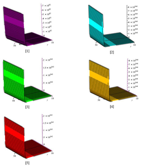
Figure 1. The plots of $\underset{i=1,\cdots ,5}{\underbrace{{\phi }_1^{Ⓢ}}}$, for $\wp =0.10$.

Table 1. The numerical results of $\underset{i=1,\cdots ,5}{\underbrace{{\phi }_1^{Ⓢ}}}$, for $\wp =0.10$.

X	0.10	0.50	3	5
${\phi }_1^{Ⓢ}\left(X\right)$	1.0106	2.0770	9.8802	9.6986
${\phi }_2^{Ⓢ}\left(X\right)$	0.0105	0.4146	2.8577	9.0706
${\phi }_3^{Ⓢ}\left(X\right)$	0.9998	0.7113	1.2060	2.0432
${\phi }_4^{Ⓢ}\left(X\right)$	0.0105	0.7840	4.0936	9.1747
${\phi }_5^{Ⓢ}\left(X\right)$	1.0001	1.3656	1.7264	2.3222

3. UHS for (5), under Conditions (2)

Here, we present the general concept of the UHS of an operator equation. Let $(\mathcal{V},\mathcal{F},{\otimes }_{\mathcal{M}})$ be an MVFB-space and $\varnothing \ne \mathcal{W}\subseteq \mathcal{V},$ and $\mathcal{L}$ be an operator from $\mathcal{W}$ to $\mathcal{V}$. Consider the operator equation

$$\begin{array}{c}\hfill \mathcal{L}\left(v\right)=0,\forall v\in \mathcal{W},\end{array}$$

(26)

and

$$\begin{array}{c}\hfill \mathcal{F}(\mathcal{L}\left(w\right),\overrightarrow{\mu })⪰\mathcal{F}(ϵ,\overrightarrow{\mu }),\forall ϵ>0,w\in \mathcal{W},\end{array}$$

(27)

where $\overrightarrow{\mu }>\overrightarrow{0}.$ Equation (26) is UHS, if for every solution ${\varpi }_1$ of (27) there is a solution ${\varpi }_2$ of Equation (26), s.t.

$$\begin{array}{c}\hfill \mathcal{F}({\varpi }_1-{\varpi }_2,\overrightarrow{\mu })⪰\mathcal{F}(cϵ,\overrightarrow{\mu }),\forall c>0,\end{array}$$

where $\overrightarrow{\mu }>\overrightarrow{0}.$

Theorem 2.

If each eigenvalue of ζ satisfies $|arg(\xi \left(\zeta \right)\left)\right|>0.5\wp \pi ,$ then Equation (5) is UHS.

Proof. 

We see that the only solution of (5) is

$$\begin{array}{c}\hfill {\lambda }_1(\propto )=M_{\wp }\left(\zeta {\propto }^{\wp }\right){\propto }_0+{\int }_0^{\propto }{(\propto -{\propto }^{\prime })}^{\wp -1}{M}_{\wp }\left(\zeta {(\propto -{\propto }^{\prime })}^{\wp }\right){\lambda }_2\left({\propto }^{\prime }\right)d{\propto }^{\prime };\end{array}$$

(28)

for more details we refer the reader to [15]. Now, consider the inequality

$$\begin{array}{c}\hfill \mathcal{F}\left({}^{\mathcal{H}}{\mathbf{D}}^{\wp ,\gamma }{\lambda }_1(\propto )-\zeta {\lambda }_1(\propto )-{\lambda }_2(\propto ),\overrightarrow{\mu }\right)⪰\mathcal{F}(\mathcal{S},\overrightarrow{\mu }),\end{array}$$

(29)

where $\mathcal{S}>0.$

Based on Remark 1.7 in [16] and Remark 1 in [17], a mapping $\widehat{{\lambda }_1}$ is a solution of (29), iff there is a mapping ${ð}^{*}\in {\eta }_{n,1}$ s.t.:

(1)

$\mathcal{F}({ð}^{*}(\propto ),\overrightarrow{\mu })⪰\mathcal{F}(\mathcal{S},\overrightarrow{\mu })$, for all $\propto \in (0,\bigwedge )$.

(2)

We get

$$\begin{array}{c}\hfill {}^{\mathcal{H}}{\mathbf{D}}^{\wp ,\gamma }\widehat{{\lambda }_1}(\propto )=\zeta \widehat{{\lambda }_1}(\propto )+{\lambda }_2(\propto )+{ð}^{*}(\propto ).\end{array}$$

(30)

Therefore, $\widehat{{\lambda }_1}$ is a solution of the inequality

$$\begin{array}{ccc}& & \mathcal{F}\left(\widehat{{\lambda }_1}(\propto )-M_{\wp }\left(\zeta {\propto }^{\wp }\right){\propto }_0-{\int }_0^{\propto }{(\propto -{\propto }^{\prime })}^{\wp -1}{M}_{\wp }\left(\zeta {(\propto -{\propto }^{\prime })}^{\wp }\right){\lambda }_2\left({\propto }^{\prime }\right)d{\propto }^{\prime },\overrightarrow{\mu }\right)\hfill \\ & ⪰& \mathcal{F}({\mathcal{S}}^{\prime },\overrightarrow{\mu }),\hfill \end{array}$$

(31)

where ${\mathcal{S}}^{\prime }>0.$

According to (24), we get

$\widehat{{\lambda }_1}(\propto )=M_{\wp }\left(\zeta {\propto }^{\wp }\right){\propto }_0+{\int }_0^{\propto }{(\propto -{\propto }^{\prime })}^{\wp -1}{M}_{\wp }\left(\zeta {(\propto -{\propto }^{\prime })}^{\wp }\right)[{\lambda }_2\left({\propto }^{\prime }\right)+{ð}^{*}\left({\propto }^{\prime }\right)]d{\propto }^{\prime }$.

Then,

$$\begin{array}{ccc}\hfill & & \mathcal{F}\left(\widehat{{\lambda }_1}(\propto )-M_{\wp }\left(\zeta {\propto }^{\wp }\right){\propto }_0-{\int }_0^{\propto }{(\propto -{\propto }^{\prime })}^{\wp -1}{M}_{\wp }\left(\zeta {(\propto -{\propto }^{\prime })}^{\wp }\right){\lambda }_2\left({\propto }^{\prime }\right)d{\propto }^{\prime },\overrightarrow{\mu }\right)\hfill \\ & & =\mathcal{F}\left({\int }_0^{\propto }{(\propto -{\propto }^{\prime })}^{\wp -1}{M}_{\wp }\left(\zeta {(\propto -{\propto }^{\prime })}^{\wp }\right){ð}^{*}\left({\propto }^{\prime }\right)d{\propto }^{\prime },\overrightarrow{\mu }\right)\hfill \\ & & =\mathcal{F}\left({\int }_0^{\propto }{\left({\propto }^{\prime }\right)}^{\wp -1}{M}_{\wp }\left(\zeta {\left({\propto }^{\prime }\right)}^{\wp }\right){ð}^{*}(\propto -{\propto }^{\prime })d{\propto }^{\prime },\overrightarrow{\mu }\right)\hfill \\ & & ⪰\mathcal{F}\left(\mathcal{S}{\int }_0^{\propto }{\left({\propto }^{\prime }\right)}^{\wp -1}{M}_{\wp }\left(\zeta {\left({\propto }^{\prime }\right)}^{\wp }\right)d{\propto }^{\prime },\overrightarrow{\mu }\right).\hfill \end{array}$$

(32)

Assume any eigenvalue of $\zeta$ satisfies $|arg\left(\xi \left(\zeta \right)\right)|>{\displaystyle \frac{\wp \pi }{2}}.$ Additionally, suppose the matrix $\zeta$ is diagonalizable. Then, there is a matrix P, s.t.

$${\mathfrak{C}}_1=P^{-1}\zeta P=\mathrm{diag}({\xi }_1,\dots ,{\xi }_n).$$

Therefore,

$$M_{\wp }\left(\zeta {\left({\propto }^{\prime }\right)}^{\wp }\right)=P{M}_{\wp }\left({\mathfrak{C}}_1{\left({\propto }^{\prime }\right)}^{\wp }\right)P^{-1}=P\mathrm{diag}[M_{\wp }\left({\xi }_1{\left({\propto }^{\prime }\right)}^{\wp }\right),\dots ,M_{\wp }\left({\xi }_n{\left({\propto }^{\prime }\right)}^{\wp }\right)]P^{-1},$$

and

$$\begin{array}{ccc}& & \mathcal{F}\left({\int }_0^{\propto }{\left({\propto }^{\prime }\right)}^{\wp -1}{M}_{\wp }\left(\zeta {\left({\propto }^{\prime }\right)}^{\wp }\right)d{\propto }^{\prime },\frac{\overrightarrow{\mu }}{\mathcal{S}}\right)\hfill \\ & & =\mathcal{F}\left({\int }_0^{\propto }P\mathrm{diag}[{\left({\propto }^{\prime }\right)}^{\wp -1}{M}_{\wp }\left({\xi }_1{\left({\propto }^{\prime }\right)}^{\wp }\right),\dots ,{\left({\propto }^{\prime }\right)}^{\wp -1}{M}_{\wp }\left({\xi }_n{\left({\propto }^{\prime }\right)}^{\wp }\right)]P^{-1}d{\propto }^{\prime },\frac{\overrightarrow{\mu }}{\mathcal{S}}\right).\hfill \end{array}$$

We claim there is a $c>0,$ s.t.

$$\mathcal{F}\left({\int }_0^{\propto }{\left({\propto }^{\prime }\right)}^{\wp -1}{M}_{\wp }\left({\xi }_i{\left({\propto }^{\prime }\right)}^{\wp }\right)d{\propto }^{\prime },\overrightarrow{\mu }\right)⪰\mathcal{F}(c,\overrightarrow{\mu }).$$

According to (15), we find for ∝ > ${\propto }_0$ (>0),

$$\begin{array}{ccc}& & \mathcal{F}\left({\int }_0^{\propto }{\left({\propto }^{\prime }\right)}^{\wp -1}{M}_{\wp }\left({\xi }_i{\left({\propto }^{\prime }\right)}^{\wp }\right)d{\propto }^{\prime },\frac{\overrightarrow{\mu }}{\mathcal{S}}\right)\hfill \\ & & =\mathcal{F}\left({\int }_0^{{\propto }_0}{\left({\propto }^{\prime }\right)}^{\wp -1}{M}_{\wp }\left({\xi }_i{\left({\propto }^{\prime }\right)}^{\wp }\right)d{\propto }^{\prime },\frac{\overrightarrow{\mu }}{2\mathcal{S}}\right)\otimes \mathcal{F}\left({\int }_{{\propto }_0}^{\propto }{\left({\propto }^{\prime }\right)}^{\wp -1}{M}_{\wp }\left({\xi }_i{\left({\propto }^{\prime }\right)}^{\wp }\right)d{\propto }^{\prime },\frac{\overrightarrow{\mu }}{2\mathcal{S}}\right)\hfill \\ & & =\mathcal{F}\left({\int }_0^{{\propto }_0}{\left({\propto }^{\prime }\right)}^{\wp -1}{M}_{\wp }\left({\xi }_i{\left({\propto }^{\prime }\right)}^{\wp }\right)d{\propto }^{\prime },\frac{\overrightarrow{\mu }}{2\mathcal{S}}\right)\hfill \\ & & \otimes \mathcal{F}\left({\int }_{{\propto }_0}^{\propto }{\left({\propto }^{\prime }\right)}^{\wp -1}[-\sum _{k=2}^p\frac{{\left({\xi }_i{\left({\propto }^{\prime }\right)}^{\wp }\right)}^{-k}}{\Gamma (1-\wp k)}+O\left(\right|{\xi }_i{\left({\propto }^{\prime }\right)}^{\wp }{|}^{-1-p}\left)\right]d{\propto }^{\prime },\frac{\overrightarrow{\mu }}{2\mathcal{S}}\right)\hfill \\ & & =\mathcal{F}\left({\int }_0^{{\propto }_0}{\left({\propto }^{\prime }\right)}^{\wp -1}{M}_{\wp }\left({\xi }_i{\left({\propto }^{\prime }\right)}^{\wp }\right)d{\propto }^{\prime },\frac{\overrightarrow{\mu }}{2\mathcal{S}}\right)\hfill \\ & & \otimes \mathcal{F}\left({\int }_{{\propto }_0}^{\propto }[-\sum _{k=2}^p\frac{{\left({\xi }_i\right)}^{-k}{\left({\propto }^{\prime }\right)}^{-\wp k+\wp -1}}{\Gamma (1-\wp k)}+O\left(\right|{\xi }_i{|}^{-1-p}{\left({\propto }^{\prime }\right)}^{-\wp p-1}]d{\propto }^{\prime },\frac{\overrightarrow{\mu }}{2\mathcal{S}}\right)\hfill \\ & & ⪰\mathcal{F}\left({\int }_0^{{\propto }_0}{\left({\propto }^{\prime }\right)}^{\wp -1}{M}_{\wp }\left(\right|{\xi }_i\left|{\left({\propto }^{\prime }\right)}^{\wp }\right)d{\propto }^{\prime },\frac{\overrightarrow{\mu }}{2\mathcal{S}}\right)\hfill \\ & & \otimes \mathcal{F}\left({\int }_{{\propto }_0}^{\propto }[\sum _{k=2}^p\frac{|{\xi }_i{|}^{-k}{\left({\propto }^{\prime }\right)}^{-\wp k+\wp -1}}{|\Gamma (1-\wp k\left)\right|}+O\left(\right|{\xi }_i{|}^{-1-p}{\left({\propto }^{\prime }\right)}^{-\wp p-1}]d{\propto }^{\prime },\frac{\overrightarrow{\mu }}{2\mathcal{S}}\right)\hfill \\ & & =\mathcal{F}\left(\sum _{k=0}^{\infty }\frac{|{\xi }_i{|}^k}{\Gamma (\wp k+1)}{\int }_0^{{\propto }_0}{\left({\propto }^{\prime }\right)}^{\wp k+\wp -1}d{\propto }^{\prime },\frac{\overrightarrow{\mu }}{2\mathcal{S}}\right)\hfill \\ & & \otimes \mathcal{F}\left(\sum _{k=2}^p\frac{|{\xi }_i{|}^{-k}}{|\Gamma (1-\wp k\left)\right|}{\int }_{{\propto }_0}^{\propto }{\left({\propto }^{\prime }\right)}^{-\wp k+\wp -1}d{\propto }^{\prime }+O\left(\right|{\xi }_i{\left|\right)}^{-1-p}{\propto }^{-\wp p},\frac{\overrightarrow{\mu }}{2\mathcal{S}}\right)\hfill \\ & & =\mathcal{F}\left(\sum _{k=0}^{\infty }\frac{|{\xi }_i{|}^k{\propto }_0^{\wp k+\wp }}{\Gamma (\wp k+2)},\frac{\overrightarrow{\mu }}{2\mathcal{S}}\right)\hfill \\ & & \otimes \mathcal{F}\left(\sum _{k=2}^p\frac{|{\xi }_i{|}^{-k}{\propto }^{-\wp k+\wp }}{(-\wp k+1)|\Gamma (1-\wp k\left)\right|}-\sum _{k=2}^p\frac{|{\xi }_i{|}^{-k}{\propto }_0^{-\wp k+\wp }}{(-\wp k+1)|\Gamma (1-\wp k\left)\right|}+O\left(\right|{\xi }_i{|}^{-1-p}{\propto }^{-\wp p}),\frac{\overrightarrow{\mu }}{2\mathcal{S}}\right)\hfill \\ & & ⟶\mathcal{F}\left({\propto }_0^{\wp }{M}_{\wp ,2}\left(\right|{\xi }_i\left|{\propto }_0^{\wp }\right),\frac{\overrightarrow{\mu }}{2\mathcal{S}}\right)\otimes \mathcal{F}\left(\sum _{k=2}^p\frac{|{\xi }_i{|}^{-k}{\propto }_0^{-\wp k+\wp }}{\Gamma (2-\wp k)},\frac{\overrightarrow{\mu }}{2\mathcal{S}}\right)\mathrm{as}\propto ⟶\infty ,\hfill \end{array}$$

where $\overrightarrow{\mu }>\overrightarrow{0}.$ Therefore, there is a ${\mathcal{S}}^{\prime }>0,$ s.t. $\mathcal{F}\left({\int }_0^{\propto }{\left({\propto }^{\prime }\right)}^{\wp -1}{M}_{\wp }\left(\xi {\left({\propto }^{\prime }\right)}^{\wp }\right)d{\propto }^{\prime },\overrightarrow{\mu }\right)⪰\mathcal{F}({\mathcal{S}}^{\prime },\overrightarrow{\mu }),$ for every $\overrightarrow{\mu }>\overrightarrow{0}.$

Now, assume $\zeta$ is a Jordan form, i.e., there is a matrix P s.t.

$${\mathfrak{C}}_2=P^{-1}\zeta P=\mathrm{diag}({\mathfrak{C}}_{21},\dots ,{\mathfrak{C}}_{2r}),$$

in which ${\mathfrak{C}}_{2i},1\le i\le r$ is given by

$${\left[\begin{array}{cccc}{\xi }_i& 1& & \\ & {\xi }_i& \ddots & \\ & & \ddots & 1\\ & & & {\xi }_i\end{array}\right]}_{n_i\times n_i},$$

and also ${\sum }_{i=1}^r{n}_i=n.$ We get

$$M_{\wp }\left(\zeta {\left({\propto }^{\prime }\right)}^{\wp }\right)=P\mathrm{diag}[M_{\wp }\left({\mathfrak{C}}_{21}{\left({\propto }^{\prime }\right)}^{\wp }\right),\dots ,M_{\wp }\left({\mathfrak{C}}_{2r}{\left({\propto }^{\prime }\right)}^{\wp }\right)]P^{-1},1\le i\le r,$$

and

$$\begin{array}{ccc}& & M_{\wp }\left({\mathfrak{C}}_{2i}{\left({\propto }^{\prime }\right)}^{\wp }\right)\hfill \\ & =& \sum _{k=0}^{\infty }{\displaystyle \frac{{\left({\mathfrak{C}}_{2i}{\left({\propto }^{\prime }\right)}^{\wp }\right)}^k}{\Gamma (\wp k+1)}}\hfill \\ & =& \sum _{k=0}^{\infty }{\displaystyle \frac{{\left({\left({\propto }^{\prime }\right)}^{\wp }\right)}^k}{\Gamma (\wp k+1)}}{\mathfrak{C}}_{2i}^k\hfill \\ & =& \sum _{k=0}^{\infty }{\displaystyle \frac{{\left({\left({\propto }^{\prime }\right)}^{\wp }\right)}^k}{\Gamma (\wp k+1)}}\left[\begin{array}{ccc}{\xi }_i^k{C}_k^1{\xi }_i^{k-1}& \dots & C_k^{n_i-1}{\xi }_i^{k-n_i-1}\\ {\xi }_i^k& \ddots & ⋮\\ & \ddots & C_k^1{\xi }_i^{k-1}\\ & & {\xi }_i^k\end{array}\right]\hfill \\ & =& \left[\begin{array}{cccc}\sum _{k=0}^{\infty }{\displaystyle \frac{{\left({\xi }_i{\left({\propto }^{\prime }\right)}^{\wp }\right)}^k}{\Gamma (\wp k+1)}}& \sum _{k=0}^{\infty }{\displaystyle \frac{{\left({\propto }^{\prime }\right)}^{\wp k}}{\Gamma (\wp k+1)}}{C}_k^1{\xi }_i^{k-1}& \dots & \sum _{k=0}^{\infty }{\displaystyle \frac{{\left({\propto }^{\prime }\right)}^{\wp k}}{\Gamma (\wp k+1)}}{C}_k^{n_i-1}{\xi }_i^{k-n_i+1}\\ & \sum _{k=0}^{\infty }{\displaystyle \frac{{\left({\xi }_i{\left({\propto }^{\prime }\right)}^{\wp }\right)}^k}{\Gamma (\wp k+1)}}& \ddots & ⋮\\ & & \ddots & \sum _{k=0}^{\infty }{\displaystyle \frac{{\left({\propto }^{\prime }\right)}^{\wp k}}{\Gamma (\wp k+1)}}{C}_k^1{\xi }_i^{k-1}\\ & & & \sum _{k=0}^{\infty }{\displaystyle \frac{{\left({\xi }_i{\left({\propto }^{\prime }\right)}^{\wp }\right)}^k}{\Gamma (\wp k+1)}}\end{array}\right]\hfill \\ & =& \left[\begin{array}{cccc}{M}_{\wp }\left({\xi }_i{\left({\propto }^{\prime }\right)}^{\wp }\right)& {\displaystyle \frac{1}{1!}}{\displaystyle \frac{\partial }{\partial {\xi }_i}}{M}_{\wp }\left({\xi }_i{\left({\propto }^{\prime }\right)}^{\wp }\right)& \dots & {\displaystyle \frac{1}{(n_i-1)!}}{\left({\displaystyle \frac{\partial }{\partial {\xi }_i}}\right)}^{n_i-1}{M}_{\wp }\left({\xi }_i{\left({\propto }^{\prime }\right)}^{\wp }\right)\\ & M_{\wp }\left({\xi }_i{\left({\propto }^{\prime }\right)}^{\wp }\right)& \ddots & ⋮\\ & & \ddots & {\displaystyle \frac{1}{1!}}{\displaystyle \frac{\partial }{\partial {\xi }_i}}{M}_{\wp }\left({\xi }_i{\left({\propto }^{\prime }\right)}^{\wp }\right)\\ & & & M_{\wp }\left({\xi }_i{\left({\propto }^{\prime }\right)}^{\wp }\right),\end{array}\right]\hfill \end{array}$$

in which $C_k^m,1\le m\le n_i-1$ are said to be binomial coefficients. For ∝ > ${\propto }_0$ (>0), we get

$$\begin{array}{ccc}& & \mathcal{F}\left({\int }_0^{\propto }{\left({\propto }^{\prime }\right)}^{\wp -1}\frac{1}{m!}{\left(\frac{\partial }{\partial {\xi }_i}\right)}^m{M}_{\wp }\left({\xi }_i{\left({\propto }^{\prime }\right)}^{\wp }\right)d{\propto }^{\prime },\frac{\overrightarrow{\mu }}{\mathcal{S}}\right)\hfill \\ & & =\mathcal{F}\left({\int }_0^{{\propto }_0}{\left({\propto }^{\prime }\right)}^{\wp -1}\frac{1}{m!}{\left(\frac{\partial }{\partial {\xi }_i}\right)}^m{M}_{\wp }\left({\xi }_i{\left({\propto }^{\prime }\right)}^{\wp }\right)d{\propto }^{\prime },\frac{\overrightarrow{\mu }}{\mathcal{S}}\right)\hfill \\ & & \otimes \mathcal{F}\left({\int }_{{\propto }_0}^{\propto }{\left({\propto }^{\prime }\right)}^{\wp -1}\frac{1}{m!}{\left(\frac{\partial }{\partial {\xi }_i}\right)}^m{M}_{\wp }\left({\xi }_i{\left({\propto }^{\prime }\right)}^{\wp }\right)d{\propto }^{\prime },\frac{\overrightarrow{\mu }}{2\mathcal{S}}\right)\hfill \\ & & ⪰\mathcal{F}\left({\int }_0^{{\propto }_0}\sum _{k=0}^{\infty }\frac{{(-1+k)k\dots (1-m+k)\left|\xi \right|}^{-m+k}{\left({\propto }^{\prime }\right)}^{\wp k+\wp -1}}{\Gamma (1+\wp k)m!}d{\propto }^{\prime },\frac{\overrightarrow{\mu }}{2\mathcal{S}}\right)\hfill \\ & & \otimes \mathcal{F}\left({\int }_{{\propto }_0}^{\propto }\frac{1}{m!}{\left(\frac{\partial }{\partial {\xi }_i}\right)}^m{\left({\propto }^{\prime }\right)}^{\wp -1}\{-\sum _{k=2}^p\frac{{\left({\xi }_i{\left({\propto }^{\prime }\right)}^{\wp }\right)}^{-k}}{\Gamma (-\wp k+1)}+O\left(\right|{\xi }_i{\left({\propto }^{\prime }\right)}^{\wp }{|}^{-p-1}\left)\right\}d{\propto }^{\prime },\frac{\overrightarrow{\mu }}{2\mathcal{S}}\right)\hfill \\ & & =\mathcal{F}\left(\sum _{k=0}^{\infty }\frac{{(k-1)k\dots (1-m+k)\left|\xi \right|}^{-m+k}}{\Gamma (1+\wp k)m!}{\int }_0^{{\propto }_0}{\left({\propto }^{\prime }\right)}^{-1+\wp +\wp k}d{\propto }^{\prime },\frac{\overrightarrow{\mu }}{2\mathcal{S}}\right)\hfill \\ & \otimes & \mathcal{F}({\int }_{{\propto }_0}^{\propto }{\left({\propto }^{\prime }\right)}^{\wp -1}\{-\sum _{k=2}^p\frac{(-1+m+k)!{(-1)}^m{\xi }_i^{-m-k}{\left({\propto }^{\prime }\right)}^{-k\wp }}{m!(k-1)!\Gamma (-k\wp +1)}\hfill \\ & & +O\left(\right|{\xi }_i{|}^{-1-m-p}{\left({\propto }^{\prime }\right)}^{(-p-1)\wp }\left)\right\}d{\propto }^{\prime },\frac{\overrightarrow{\mu }}{2\mathcal{S}})\hfill \\ & & ⪰\mathcal{F}\left(\sum _{k=0}^{\infty }\frac{{(k-1)k\dots (1-m+k)\left|\xi \right|}^{-m+k}{\propto }_0^{\wp +\wp k}}{\Gamma (\wp k+2)m!},\frac{\overrightarrow{\mu }}{2\mathcal{S}}\right)\hfill \\ & & \otimes \mathcal{F}({\int }_{{\propto }_0}^{\propto }\{\sum _{k=2}^p\frac{(-1+m-k)!{\xi }_i^{-m-k}{\left({\propto }^{\prime }\right)}^{-1-\wp k+\wp }}{(-1+k)!m!|\Gamma (-\wp k+1\left)\right|}\hfill \\ & & +O\left(\right|{\xi }_i{|}^{-m-p-1}{\left({\propto }^{\prime }\right)}^{-1-\wp p}\left)\right\}d{\propto }^{\prime },\frac{\overrightarrow{\mu }}{2\mathcal{S}})\hfill \\ & & =\mathcal{F}\left({\propto }_0^{\wp }\frac{1}{m!}{\left(\frac{\partial }{\partial |{\xi }_i|}\right)}^m{M}_{\wp ,2}\left(\right|{\xi }_i|{\propto }_0^{\wp })+O(|{\xi }_i{|}^{-p-1-m}{\propto }^{-\wp p}),\frac{\overrightarrow{\mu }}{2\mathcal{S}}\right)\hfill \\ & & \otimes \mathcal{F}\left(\sum _{k=2}^p\frac{(-1+k+m)!{\xi }_i^{-k-m}}{m!(k-1)!|\Gamma (-\wp k+1\left)\right|}\{\frac{{\propto }^{-\wp k+\wp }}{-\wp k+\wp }-\frac{{\propto }_0^{-\wp k+\wp }}{-\wp k+\wp }\},\frac{\overrightarrow{\mu }}{2\mathcal{S}}\right)\hfill \\ & & ⟶\mathcal{F}\left({\propto }_0^{\wp }\frac{1}{m!}{\left(\frac{\partial }{\partial |{\xi }_i|}\right)}^m{M}_{\wp ,2}\left(\right|{\xi }_i\left|{\propto }_0^{\wp }\right),\frac{\overrightarrow{\mu }}{2\mathcal{S}}\right)\hfill \\ & & \otimes \mathcal{F}\left(\sum _{k=2}^p\frac{(-1+k+m)!|{\xi }_i{|}^{-k-m}{\propto }_0^{\wp -\wp k}}{m!(k-1)!|\Gamma (2-\wp k\left)\right|},\frac{\overrightarrow{\mu }}{2\mathcal{S}}\right),\mathrm{as}\propto ⟶\infty ,\hfill \end{array}$$

where $1\le m\le n_i-1.$ Therefore, there is a ${\mathcal{S}}^{\prime }>0,$ s.t.

$$\mathcal{F}\left({\int }_0^{\propto }{\left({\propto }^{\prime }\right)}^{\wp -1}{M}_{\wp }\left(\xi {\left({\propto }^{\prime }\right)}^{\wp }\right)d{\propto }^{\prime },\overrightarrow{\mu }\right)⪰\mathcal{F}({\mathcal{S}}^{\prime },\overrightarrow{\mu }).$$

Now, (28) and (32) imply that there is a constant c > 0 s.t.

$$\mathcal{F}({\lambda }_1(\propto )-\widehat{{\lambda }_1}(\propto ),\overrightarrow{\mu })⪰\mathcal{F}(c,\overrightarrow{\mu }),$$

for any $\overrightarrow{\mu }>\overrightarrow{0}.$ Thus, system (5) is UHS. □

4. UHS for (5), under Conditions (3)

Theorem 3.

If any eigenvalue of ζ satisfies $|arg\left(\xi \left(\zeta \right)\right)|>{\displaystyle \frac{\wp \pi }{2}},$ then (5) is UHS.

Proof. 

We see that the only solution of (5) is

$$\begin{array}{c}\hfill {\lambda }_1(\propto )=M_{\wp }\left(\zeta {\propto }^{\wp }\right){\propto }_0+{\int }_0^{\propto }{(\propto -{\propto }^{\prime })}^{\wp -1}{M}_{\wp }\left(\zeta {(\propto -{\propto }^{\prime })}^{\wp }\right){\lambda }_2\left({\propto }^{\prime }\right)d{\propto }^{\prime }.\end{array}$$

(33)

Now, consider the following inequality,

$$\begin{array}{ccc}\hfill & & \mathcal{F}\left({}^{\mathcal{H}}{\mathbf{D}}^{\wp ,\gamma }{\lambda }_1(\propto )-\zeta {\lambda }_1(\propto )-{\lambda }_2(\propto ),\overrightarrow{\mu }\right)\hfill \\ & ⪰& \mathcal{F}(\mathcal{S},\overrightarrow{\mu }),\hfill \end{array}$$

(34)

where $\mathcal{S}>0.$

A mapping $\widehat{{\lambda }_1}$ is a solution of (34), iff there is a mapping ${ð}^{*}\in {\eta }_{n,m}$ s.t.:

(1)

$\mathcal{F}(\overrightarrow{\mu },{ð}^{*}(\propto ))⪰\mathcal{F}(\mathcal{S},\overrightarrow{\mu })$, for all $\propto \in (0,\bigwedge )$.

(2)

We have

$$\begin{array}{c}\hfill {}^{\mathcal{H}}{\mathbf{D}}^{\wp ,\gamma }\widehat{{\lambda }_1}(\propto )=\zeta \widehat{{\lambda }_1}(\propto )+{\lambda }_2(\propto )+{ð}^{*}(\propto ).\end{array}$$

(35)

Then, $\widehat{{\lambda }_1}$ is a solution of the following inequality,

$$\begin{array}{ccc}& & \mathcal{F}\left(-M_{\wp }\left(\zeta {\propto }^{\wp }\right){\propto }_0+\widehat{{\lambda }_1}(\propto )-{\int }_0^{\propto }{(\propto -{\propto }^{\prime })}^{\wp -1}{M}_{\wp }\left(\zeta {(-{\propto }^{\prime }+\propto )}^{\wp }\right){\lambda }_2\left({\propto }^{\prime }\right)d{\propto }^{\prime },\overrightarrow{\mu }\right)\hfill \\ & ⪰& \mathcal{F}({\mathcal{S}}^{″},\overrightarrow{\mu }),\hfill \end{array}$$

(36)

where ${\mathcal{S}}^{″}>0.$

According to (35),

$$\widehat{{\lambda }_1}(\propto )={\int }_0^{\propto }{(\propto -{\propto }^{\prime })}^{\wp -1}{M}_{\wp }\left(\zeta {(\propto -{\propto }^{\prime })}^{\wp }\right)[{\lambda }_2\left({\propto }^{\prime }\right)+{ð}^{*}\left({\propto }^{\prime }\right)]d{\propto }^{\prime }+M_{\wp }\left(\zeta {\propto }^{\wp }\right){\propto }_0.$$

Consequently,

$$\begin{array}{ccc}& & \mathcal{F}\left(\widehat{{\lambda }_1}(\propto )-M_{\wp }\left(\zeta {\propto }^{\wp }\right){\propto }_0-{\int }_0^{\propto }{(-{\propto }^{\prime }+\propto )}^{\wp -1}{M}_{\wp }\left(\zeta {(\propto -{\propto }^{\prime })}^{\wp }\right){\lambda }_2\left({\propto }^{\prime }\right)d{\propto }^{\prime },\overrightarrow{\mu }\right)\hfill \\ & & =\mathcal{F}\left({\int }_0^{\propto }{(-{\propto }^{\prime }+\propto )}^{\wp -1}{M}_{\wp }\left(\zeta {(\propto -{\propto }^{\prime })}^{\wp }\right){ð}^{*}\left({\propto }^{\prime }\right)d{\propto }^{\prime },\overrightarrow{\mu }\right)\hfill \\ & & =\mathcal{F}\left({\int }_0^{\propto }{\left({\propto }^{\prime }\right)}^{\wp -1}{M}_{\wp }\left(\zeta {\left({\propto }^{\prime }\right)}^{\wp }\right){ð}^{*}(-{\propto }^{\prime }+\propto )d{\propto }^{\prime },\overrightarrow{\mu }\right)\hfill \\ & & ⪰\mathcal{F}\left(\mathcal{S}{\int }_0^{\propto }{\left({\propto }^{\prime }\right)}^{\wp -1}{M}_{\wp }\left(\zeta {\left({\propto }^{\prime }\right)}^{\wp }\right)d{\propto }^{\prime },\overrightarrow{\mu }\right)\hfill \\ & & ⪰\mathcal{F}({\mathcal{S}}^{″},\overrightarrow{\mu }),\hfill \end{array}$$

where ${\mathcal{S}}^{″}>0.$ □

5. UHS for (5), under Conditions (4)

Theorem 4.

Assume that any eigenvalue of ζ and $\overline{\zeta }$ satisfy

$$0.5\pi \wp <k<min\{\pi \wp ,\pi \},\pi \ge |arg\left(\xi \left(\overline{\zeta }\right)\right)|\ge k,|arg\left(\xi \left(\zeta \right)\right)|>0.5\pi \wp .$$

Then, (5) is UHS.

Proof. 

We see that the only solution of Equation (5) is

$$\begin{array}{ccc}\hfill {\lambda }_1(\propto )& =& M_{\wp }\left(\zeta {\propto }^{\wp }\right){\propto }_0{M}_{\wp }\left(\overline{\zeta }{\propto }^{\wp }\right)\hfill \end{array}$$

(37)

$$\begin{array}{ccc}& +& {\int }_0^{\propto }{(-{\propto }^{\prime }+\propto )}^{\wp -1}{M}_{\wp }\left(\zeta {(-{\propto }^{\prime }+\propto )}^{\wp }\right){\lambda }_2\left({\propto }^{\prime }\right)M_{\wp }\left(\overline{\zeta }{(-{\propto }^{\prime }+\propto )}^{\wp }\right)d{\propto }^{\prime }.\hfill \end{array}$$

(38)

Now, consider the following inequality,

$$\begin{array}{c}\hfill \mathcal{F}\left({}^{\mathcal{H}}{\mathbf{D}}^{\wp ,\gamma }{\lambda }_1(\propto )-\zeta {\lambda }_1(\propto )-{\lambda }_1(\propto )\overline{\zeta }-{\lambda }_2(\propto ),\overrightarrow{\mu }\right)⪰\mathcal{F}(\mathcal{S},\overrightarrow{\mu }),\end{array}$$

(39)

where $\mathcal{S}>0.$

A mapping $\widehat{{\lambda }_1}$ is a solution of (39), iff there is a mapping ${ð}^{*}\in {\eta }_{n,m}$ s.t.:

(1)

$\mathcal{F}\left({ð}^{*}(\propto ),\overrightarrow{\mu }\right)⪰\mathcal{F}(\mathcal{S},\overrightarrow{\mu })$, for all $\propto \in (0,\bigwedge )$.

(2)

We get

$$\begin{array}{c}\hfill {}^{\mathcal{H}}{\mathbf{D}}^{\wp ,\gamma }\widehat{{\lambda }_1}(\propto )=\zeta \widehat{{\lambda }_1}(\propto )+\widehat{{\lambda }_1}(\propto )\overline{\zeta }+{\lambda }_2(\propto )+{ð}^{*}(\propto ).\end{array}$$

(40)

Then, $\widehat{{\lambda }_1}$ is a solution of the inequality,

$$\begin{array}{ccc}& & \mathcal{F}(-M_{\wp }\left(\zeta {\propto }^{\wp }\right){\propto }_0{M}_{\wp }\left(\overline{\zeta }{\propto }^{\wp }\right)+\widehat{{\lambda }_1}(\propto )\hfill \\ & & -{\int }_0^{\propto }{(\propto -{\propto }^{\prime })}^{\wp -1}{M}_{\wp }\left(\zeta {(\propto -{\propto }^{\prime })}^{\wp }\right){\lambda }_2\left({\propto }^{\prime }\right)M_{\wp }\left(\overline{\zeta }{(\propto -{\propto }^{\prime })}^{\wp }\right)d{\propto }^{\prime },\overrightarrow{\mu })\hfill \\ & ⪰& \mathcal{F}\left({\mathcal{S}}^{‴},\overrightarrow{\mu }\right),\hfill \end{array}$$

(41)

where ${\mathcal{S}}^{‴}>0.$

According to (40),

$$\begin{array}{ccc}\hfill \widehat{{\lambda }_1}(\propto )& =& M_{\wp }\left(\zeta {\propto }^{\wp }\right){\propto }_0{M}_{\wp }\left(\overline{\zeta }{\propto }^{\wp }\right)\hfill \\ & +& {\int }_0^{\propto }{(\propto -{\propto }^{\prime })}^{\wp -1}{M}_{\wp }\left(\zeta {(-{\propto }^{\prime }+\propto )}^{\wp }\right)[{\lambda }_2\left({\propto }^{\prime }\right)+{ð}^{*}\left({\propto }^{\prime }\right)]M_{\wp }\left(\overline{\zeta }{(-{\propto }^{\prime }+\propto )}^{\wp }\right)d{\propto }^{\prime }.\hfill \end{array}$$

According to Lemma 2, we get

$$\begin{array}{ccc}& \mathcal{F}& (\widehat{{\lambda }_1}(\propto )-M_{\wp }\left(\zeta {\propto }^{\wp }\right){\propto }_0{M}_{\wp }\left(\overline{\zeta }{\propto }^{\wp }\right)\hfill \\ & -& {\int }_0^{\propto }{(-{\propto }^{\prime }+\propto )}^{\wp -1}{M}_{\wp }\left(\zeta {(\propto -{\propto }^{\prime })}^{\wp }\right){\lambda }_2\left({\propto }^{\prime }\right)M_{\wp }\left(\overline{\zeta }{(\propto -{\propto }^{\prime })}^{\wp }\right)d{\propto }^{\prime },\overrightarrow{\mu })\hfill \\ & =& \mathcal{F}\left({\int }_0^{\propto }{(-{\propto }^{\prime }+\propto )}^{\wp -1}{M}_{\wp }\left(\zeta {(-{\propto }^{\prime }+\propto )}^{\wp }\right){ð}^{*}\left({\propto }^{\prime }\right)M_{\wp }\left(\overline{\zeta }{(-{\propto }^{\prime }+\propto )}^{\wp }\right)d{\propto }^{\prime },\overrightarrow{\mu }\right)\hfill \\ & =& \mathcal{F}\left({\int }_0^{\propto }{\left({\propto }^{\prime }\right)}^{\wp -1}{M}_{\wp }\left(\zeta {\left({\propto }^{\prime }\right)}^{\wp }\right){ð}^{*}(-{\propto }^{\prime }+\propto )M_{\wp }\left(\overline{\zeta }{\left({\propto }^{\prime }\right)}^{\wp }\right)d{\propto }^{\prime },\overrightarrow{\mu }\right)\hfill \\ & ⪰& \mathcal{F}\left(\mathcal{S}{\int }_0^{\propto }{\left({\propto }^{\prime }\right)}^{\wp -1}{M}_{\wp }\left(\zeta {\left({\propto }^{\prime }\right)}^{\wp }\right)M_{\wp }\left(\overline{\zeta }{\left({\propto }^{\prime }\right)}^{\wp }\right)d{\propto }^{\prime },\overrightarrow{\mu }\right)\hfill \\ & ⪰& \mathcal{F}\left({\int }_0^{\propto }{\left({\propto }^{\prime }\right)}^{\wp -1}{M}_{\wp }\left(\zeta {\left({\propto }^{\prime }\right)}^{\wp }\right)d{\propto }^{\prime },\frac{\overrightarrow{\mu }}{\mathcal{S}\left[{\int }_0^{\propto }{M}_{\wp }\left(\overline{\zeta }{\left({\propto }^{\prime }\right)}^{\wp }\right)d{\propto }^{\prime }\right]}\right)\hfill \\ & ⪰& \mathcal{F}\left({\mathcal{S}}^{″},\frac{\overrightarrow{\mu }}{\mathcal{S}\left[{\int }_0^{\propto }{M}_{\wp }\left(\overline{\zeta }{\left({\propto }^{\prime }\right)}^{\wp }\right)d{\propto }^{\prime }\right]}\right)\hfill \\ & ⪰& \mathcal{F}\left({\int }_0^{\propto }{M}_{\wp }\left(\overline{\zeta }{\left({\propto }^{\prime }\right)}^{\wp }\right)d{\propto }^{\prime },\frac{\overrightarrow{\mu }}{\mathcal{S}{\mathcal{S}}^{″}}\right)\hfill \\ & ⪰& \mathcal{F}\left(\frac{1}{1+\overline{\zeta }},\frac{\overrightarrow{\mu }}{\mathcal{S}{\mathcal{S}}^{″}\mathcal{C}}\right)\hfill \\ & ⪰& \mathcal{F}\left({\mathcal{S}}^{‴},\overrightarrow{\mu }\right),\hfill \end{array}$$

in which ${\mathcal{S}}^{‴}>0$ and $\mathcal{C}>0.$ □

6. Concluding Remarks

We applied some special functions (the Mittag–Leffler function in one parameter, the one parameter pre-supersine–Mittag–Leffler-type function, the one parameter pre-supercosine–Mittag–Leffler-type function, the one parameter pre-superhyperbolic supersine–Mittag–Leffler-type function, and the one parameter pre-superhyperbolic supercosine–Mittag–Leffler-type function) to present a new class of matrix-valued fuzzy controllers which enables us to propose a novel concept of stability, namely multi-stability, in matrix-valued fuzzy Banach spaces. The concept of multi-stability allows us to obtain different approximations depending on different special functions and to evaluate optimum stability and minimal errors, which enables us to obtain a unique optimal solution.

References

- Baleanu, D.; Shekari, P.; Torkzadeh, L.; Ranjbar, H.; Jajarmi, A.; Nouri, K. Stability analysis and system properties of Nipah virus transmission: A fractional calculus case study. Chaos Solitons Fractals 2023, 166, 112990. [Google Scholar] [CrossRef]
- Agarwal, R.; Sharma, U.P. Bicomplex Mittag–Leffler function and applications in integral transform and fractional calculus. In Mathematical and Computational Intelligence to Socio-Scientific Analytics and Applications; Springer: Singapore, 2023; pp. 157–167. [Google Scholar]
- Matias, G.S.; Lermen, F.H.; Matos, C.; Nicolin, D.J.; Fischer, C.; Rossoni, D.F.; Jorge, L.M. A model of distributed parameters for non-Fickian diffusion in grain drying based on the fractional calculus approach. Biosyst. Eng. 2023, 226, 16–26. [Google Scholar] [CrossRef]
- Ma, L.; Li, J. A bridge on Lomnitz type creep laws via generalized fractional calculus. Appl. Math. Model. 2023, 116, 786–798. [Google Scholar] [CrossRef]
- Hong, X.; Davodi, A.G.; Mirhosseini-Alizamini, S.M.; Khater, M.M.A.; Inc, M. New explicit solitons for the general modified fractional Degasperis–Procesi–Camassa–Holm equation with a truncated M-fractional derivative. Mod. Phys. Lett. B 2021, 35, 2150496. [Google Scholar] [CrossRef]
- Azami, R.; Ganji, D.D.; Davodi, A.G.; Babazadeh, H. Analysis of Strongly Non-linear Oscillators by Hes Improved Amplitude-Frequency Formulation. arXiv 2021, arXiv:2110.00885. [Google Scholar]
- Kahouli, O.; Makhlouf, A.B.; Mchiri, L.; Rguigui, H. Hyers–Ulam stability for a class of Hadamard fractional Itô–Doob stochastic integral equations. Chaos Solitons Fractals 2023, 166, 112918. [Google Scholar] [CrossRef]
- Ren, W.; Yang, Z.; Wang, X. A Two-branch Symmetric Domain Adaptation Neural Network Based on Ulam Stability Theory. Inf. Sci. 2023, 628, 424–438. [Google Scholar] [CrossRef]
- Benzarouala, C.; Brzdęk, J.; Oubbi, L. A fixed point theorem and Ulam stability of a general linear functional equation in random normed spaces. J. Fixed Point Theory Appl. 2023, 25, 1–38. [Google Scholar] [CrossRef]
- Narayanan, G.; Ali, M.S.; Rajchakit, G.; Jirawattanapanit, A.; Priya, B. Stability analysis for Nabla discrete fractional-order of Glucose-Insulin Regulatory System on diabetes mellitus with Mittag–Leffler kernel. Biomed. Signal Process. Control. 2023, 80, 104295. [Google Scholar] [CrossRef]
- Aderyani, S.R.; Saadati, R.; O’Regan, D. The Cădariu–Radu method for existence, uniqueness and Gauss Hypergeometric stability of a class of Ξ-Hilfer fractional differential equations. Int. J. Nonlinear Sci. Numer. Simul. 2022. [Google Scholar] [CrossRef]
- Aderyani, S.R.; Saadati, R.; Allahviranloo, T. Existence, uniqueness and matrix-valued fuzzy Mittag–LefflerHypergeometric–Wright stability for P-Hilfer fractional differential equations in matrix-valued fuzzy Banach space. Comput. Appl. Math. 2022, 41, 234. [Google Scholar] [CrossRef]
- Yang, X.J. Theory and Applications of Special Functions for Scientists and Engineers; Springer: Singapore, 2021. [Google Scholar]
- Yang, Z.; Ren, W.; Xu, T. Ulam–Hyers stability for matrix-valued fractional differential equations. J. Math. Inequal. 2018, 12, 665–675. [Google Scholar] [CrossRef]
- Aderyani, S.R.; Saadati, R.; Abdeljawad, T.; Mlaiki, N. Multi-stability of non homogenous vector-valued fractional differential equations in matrix-valued Menger spaces. Alex. Eng. J. 2022, 61, 10913–10923. [Google Scholar] [CrossRef]
- Aderyani, S.R.; Saadati, R.; Yang, X.J. Radu–Miheţ method for UHML stability for a class of ξ-Hilfer fractional differential equations in matrix valued fuzzy Banach spaces. Math. Methods Appl. Sci. 2021, 44, 14619–14631. [Google Scholar] [CrossRef]
- Wang, J.; Zhang, Y. Ulam–Hyers–Mittag–Leffler stability of fractional-order delay differential equations. Optimization 2014, 63, 1181–1190. [Google Scholar] [CrossRef]
Disclaimer/Publisher’s Note: The statements, opinions and data contained in all publications are solely those of the individual author(s) and contributor(s) and not of MDPI and/or the editor(s). MDPI and/or the editor(s) disclaim responsibility for any injury to people or property resulting from any ideas, methods, instructions or products referred to in the content. |
© 2023 by the authors. Licensee MDPI, Basel, Switzerland. This article is an open access article distributed under the terms and conditions of the Creative Commons Attribution (CC BY) license (https://creativecommons.org/licenses/by/4.0/).