Abstract
In this article, the problem of voltage and frequency stability in a hybrid multi-area power system including renewable energy sources (RES) and electric vehicles has been investigated. Fractional order systems have been used to design innovative controllers for both load frequency control (LFC) and automatic voltage regulator (AVR) based on the combination of fractional order proportional-integral and proportional-integral-derivative plus double derivative (FOPI–PIDD2). Here, the dandelion optimizer (DO) algorithm is used to optimize the proposed FOPI–PIDD2 controller to stabilize the voltage and frequency of the system. Finally, the results of simulations performed on MATLAB/Simulink show fast, stable, and robust performance based on sensitivity analysis, as well as the superiority of the proposed optimal control strategy in damping frequency fluctuations and active power, exchanged between areas when faced with step changes in load, the changes in the generation rate of units, and the uncertainties caused by the wide changes of dynamic values.
Keywords:
voltage and frequency stability; renewable energy; PIDD2 controller; FO controllers; optimization techniques; microgrid; electric vehicles MSC:
35B38; 74G65; 74H80
1. Introduction
1.1. Background and Motivation
The power system is a non-linear process that works in a constantly changing environment. Due to the nonlinearity of this system, its dynamic performance is affected by its component equipment. Therefore, the stability of this system can be studied from different perspectives. Voltage and frequency stability is a sort of power system stability that describes the power system’s capability to keep voltage and frequency within an acceptable range across the whole system both when running normally and after disruptions [1,2]. The change in active power mainly affects the frequency of the system, while reactive power depends mostly on variations in voltage and is rather insensitive to variations in frequency. Therefore, active and reactive power can be controlled separately. Currently, this topic forms the basis of the most advanced concepts for controlling large power systems [3,4,5].
One of the most complicated equipment in a power system is the synchronous generator and its controls [6,7]. The imbalance of generation and load is the most important reason for voltage and frequency instability. The dynamic performance of LFC and AVR control determines the quality of the power supply system according to frequency and voltage. The traditional controller with constant efficiency shows a weak unstable response in front of the increase of the strong fluctuating shock [8,9,10]. The application of evolutionary algorithms to find solutions to challenging real-world optimization issues has become possible as a result of advances in computer performance, and more attention has been paid to the solutions obtained in control system problems.
1.2. Literature Review
To obtain a system with an optimal dynamic response, advanced control approaches such as adaptive controllers have been used for the Egyptian power grid [11]. Linear–quadratic–Gaussian regulators have been applied for a multi-area power system with communication time delays [12,13]. Fuzzy-based controllers have been created to automatically manage the synchronous generator voltage [14,15,16]. Additionally, artificial neural networks-based AVRs are presented to enhance the transient stability limit of power system [17,18], and fractional order controllers have been used to improve the performance of the AVR system [19,20,21]. However, despite their proper efficiency in simulation, these controllers are associated with computational and structural complexities.
There are classical methods that attempt to suggest appropriate parameters using a linear and approximate model of the system. This includes evolutionary and meta-heuristic algorithms such as genetic algorithms (GA) [22,23], sine cosine [24,25], particle swarm optimization (PSO) [26,27], whale optimization algorithm [28], imperialist competitive algorithm (ICA) [29,30], teaching and learning [31], and seeker optimization (SO) [32,33]. The controller problem has become an optimization problem and by solving this problem, optimization of the controller parameters is achieved. These controllers have good performance in simulation, but it should be noted that the AVR and LFC systems are non-linear. Additionally, its parameters may change; hence, parametric and structural uncertainties are always present in these systems. These uncertainties will lead to undesirable system performance.
1.3. Contributions
In this article, an attempt is made to maintain security and return the system to a normal state by combining the AVR and LFC systems at the same time, so that based on the physical disturbances introduced at any moment, the power system returns to the initial desired state. This can be accomplished by using the recently introduced dandelion optimizer (DO), which is a novel, efficient, and nature-inspired optimization algorithm. It can be used to effectively fine-tune the proposed FOPI–PIDD2 controller, which is used to properly regulate the voltage and frequency of the multi-area power system with the presence of distributed generation. The DO imitates the lifelong journey of dandelion seeds that are carried by the wind as they grow. It has demonstrated enhanced performance in a realistic environment with various nonlinearities, as well as in improving reactive power dispatch by reducing voltage deviation and system power losses through high speed and minimal computation time [34,35]. Below is a list of DO’s primary distinctions that contribute to its supremacy [36]:
- The DO uses a different natural backdrop than other metaheuristic optimization algorithms that are already in use.
- The DO optimizer employs several tactics for the stages of exploration and exploitation. The exploration stage in the search space is guaranteed by the rising and descending stages of the DO algorithm. In contrast, the landing stage serves to promote the exploitation stage.
- In reference [36], to confirm the restricted programmability performance, DO was applied to four issues and contrasted with other techniques.
The model in our article has the advantage of incorporating actual wind speed and solar irradiance data in system modeling and investigating the effect of electric vehicles on the voltage–frequency control of a hybrid multi-area power system by considering non-linear factors to adapt to a real model. The FOPI–PIDD2 controller features an integral action with a fractional exponent, which allows it to outperform the traditional PI controller. Furthermore, optimizing the control parameters is critical for achieving rapid and dependable stability in the power system, and the DO algorithm will be employed to achieve it. The mentioned algorithm can create interaction between local and general search among the answers obtained from the answer space and also overcome local optima. The main objectives of LFC and AVR control are to keep the frequency uniform, adjust the voltage, divide the system load between the generators in an optimal and preferably economic way, adjust the power exchanged from the communication lines in the programmed values, and improve the quality of the supplied power, optimal power-sharing. The change created in the frequency and voltage of the system and the active and reactive power of the communication lines must be eliminated by the production changes in the energy sources to maintain the stability of the system. Therefore, the main contributions of the proposed method can be summarized as follows:
- Simultaneous combination of LFC and AVR control systems improves voltage and frequency fluctuations in hybrid multi-area power systems.
- The proposal of a novel combination based on combining the benefits of fractional order controllers with those of classical PID controllers whose performance is enhanced by the addition of double-derivative action, namely fractional order proportional-integral and proportional-integral-derivative plus double derivative (FOPI–PIDD2) controller. The combination of the previously mentioned efficient regulators boosts the effectiveness of stability, rapid transients, and containment of existing RES and load variations.
- Based on the recently reported nature-inspired optimization technique, the dandelion optimizer (DO), the suggested FOPI–PIDD2 controller parameters are being optimized. In addition to its remarkable iterative optimization and great resilience, the suggested DO-based optimization technique can reduce the huge training data and/or expensive mathematical computations necessary in existing methods.
- Improving the dynamic performance of the combined LFC–AVR system integrated with electric vehicles.
In the continuation, the parts of the article are as follows. In the second part, the general control structure of the voltage and frequency in multi-area power systems is described. In the third part, the proposed self-tuning control method based on the DO algorithm is introduced. In the fourth part, the simulation results are discussed. Finally, in the fifth part, the conclusion is presented.
2. Voltage and Frequency Control Infrastructure
Figure 1 shows the LFC and AVR loops simply. The aforementioned controllers are set for special operating conditions and neutralize the effect of partial changes in the load demand to keep the frequency and voltage in a certain range. Small changes in active power depend on rotor angle changes and therefore frequency, while reactive power mainly depends on voltage (generator excitation current). The time constant of the excitation system is much less than the time constant of the primary stimulus and also its transient fluctuations are damped very quickly, so it does not influence the load frequency dynamics. Therefore, the mutual effects between the LFC and the AVR loops can be ignored; hence, the analysis of load frequency control and excitation voltage control can be performed individually.
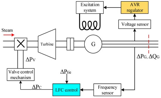
Figure 1.
AVR and LFC loop of a synchronous generator.
The change created in the system frequency and the active power of the communication lines should be eliminated by the production change. The line signals, i.e., ΔF and ΔP, are amplified and combined and then they are converted into the real command signal ΔPv which must be sent to the primary excitation to change the input power desirably. Therefore, the excitation system will also change its output power to the value of ΔPv and cause ΔF and ΔP to become insignificant.
2.1. Modeling of LFC and AVR Control System
The mathematical modelling of the control system is the initial stage in the analysis and design process. Two traditional approaches are utilized for modelling: the transform function technique and the state variable method. The method of state variables can be used for linear and non-linear systems. In order to make use of the transfer function and linear state equations, the system first has to be linearized. The oscillation equation of a synchronous generator, for a small disturbance, can be defined as Equation (1):
where H is the inertia constant in seconds, ∆δ is the rotor angle change in radians, ∆Pm is the change of mechanical power in p.u, ∆Pe is the change of electrical power in p.u, and ωs is the angular speed in radians per second. For a small deviation in speed (∆ω), Equation (1) can be expressed as Equation (2):
By putting frequency instead of angular speed, Equation (3) is obtained:
Figure 2 shows the LFC control block diagram of a separate system. According to Figure 2, Tt, Tg, and R are the steam turbine time constant, the steam governor time constant, and the governor speed regulation parameter, respectively, and D is equal to the percentage change in load compared to the percentage change in frequency. Thus, the following equations will be valid:
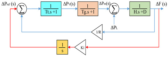
Figure 2.
The LFC control block diagram of a separate system.
Considering that the load change in the power system is generally performed by disconnecting or connecting constant values, in the LFC study, the step input is used to model the load changes. According to Figure 2, the output relation of the control system ΔF(s) in the case where ΔPc = 0 is in the form of Equation (7):
where is the power system time constant = (sec) and is the power system gain = (Hz/MW).
According to the exponential value theorem, the permanent response of the system is expressed as Equation (8):
Equation (8) shows the frequency change due to the load change where (MW/Hz) is defined as the frequency response characteristic of the area (including generator and load).
As can be seen from Equation (7), if ΔPref = 0, the change in frequency will never be zero because D is a load specification and R cannot be too small for stability reasons. When the load of the system increases, the speed of the turbine will decrease before the governor can alter the incoming steam for the recent load, and this decrease in speed, which is a decrease in the frequency of the system, will lead to a decrease in the load. Therefore, the load added to the system is compensated by two components. One is an increase in generation and the other is a decrease in the overall load of the system due to the decrease in frequency, so the frequency of the system does not return to the nominal value. However, if at the same time as the step change of the load, the speed changer is also changed in a step manner, the response of the control system is obtained as Equation (9):
Therefore, by changing the load, the speed changer can be controlled so that ΔPc = ΔPL, and as a result, the final frequency of the system can be brought to the nominal value per load change. To maintain the frequency of the system constant, the deviation of the frequency of the permanent mode, i.e., ΔF, must reach zero for a step variation in the load, and as can be seen, a speed changer is required to attain this purpose. The conventional method to push the frequency to the nominal value is to use an integrator in the form of a second feedback loop since the integral unit considers the average error for some time and can completely remove it. The red lines in Figure 2 show how to use the integrator in the LFC system. One can notice that the frequency error signal is created after amplification by the integral gain Ki through the integrator with the command ΔPc.
By applying the finite value theorem, we will have:
So, the second feedback loop reduces the frequency of exponential error to zero by increasing the degree of the system. However, the dynamic response of the system depends on the square roots of the denominator of Equation (10). By examining this equation, it is clear that by increasing the value of Ki, the speed of the response is improved, as a result of which the fluctuations increase (if Ki is increased too much, the system may become unstable) and its decrease leads to a slower response. Therefore, the integral gain should be adjusted in such a way that it creates a suitable mode for the response.
Nowadays, most power systems are connected to their neighboring areas, and the connection of the control areas creates a multi-area power system. In a multi-area power system, each control area supplies loads of its area under normal conditions, unless the power required by another area is provided by the agreement of two adjacent areas. Consider two control areas 1 and 2 in Figure 3, which are connected by a lossless communication line with reactance Xtie. According to Figure 4, each region is expressed by a voltage source and an equivalent reactance. During normal operation, the active power exchanged through the communication line is equal to Equation (12):
where X12 = X1 + Xtie + X2, δ12= δ1 − δ2. Therefore, for small deviations of transmission power around the nominal value, we have Equation (13):
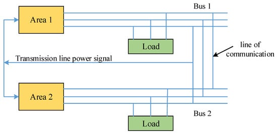
Figure 3.
Two-area power system.
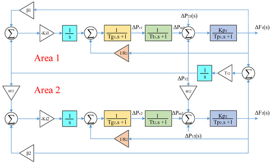
Figure 4.
LFC block diagram of a dual-area power system.
The quantity T12 is the slope of the power angle curve at the rated operating point δ120 = δ10 − Δδ20 and is called the power synchronization factor. Therefore, we have Equation (14):
So, the deviation of the power of the communication line is in the form of Equation (15).
By replacing angle changes with frequency changes and taking the Laplace transform to both sides of Equation (15), we will have:
Considering that the losses of the communication line have been omitted, ΔP12 = ΔP21 or in terms of p.u., we have:
where S1 and S2 are the rated power of areas 1 and 2 in terms of MVA. If we define the coefficient α12 according to Equation (18):
By entering the transmission power ΔP12(s) in the block diagram of area 1, we will have:
Similarly to change the frequency of area 2, we will have:
Transmission power from the communication line appears as an increase in load in one area and a decrease in load in another area. The direction of the power is determined by the difference of angles, i.e., if Δδ1 > Δδ2, the direction of the power flow will be from area 1 to area 2.
The generator’s excitation control through the use of AVR is the primary source of reactive power control for the generator. The purpose of an automatic voltage regulator (AVR) is to maintain the synchronous generator’s terminal voltage at a level that has been predetermined. A drop in the terminal voltage of a generator is observed whenever there is an increase in the reactive load power of the generator. A voltage transformer is used in one phase to make the measurement of the voltage. After being rectified, this voltage is put up against the dc setpoint signal for evaluation. The excitation terminal voltage is increased as a result of the amplified error signal, which also affects the excitation field. As a consequence of this, the excitation current of the generator is raised, which ultimately results in an increase in the quantity of emf that is generated. Because of the rise in the generation of reactive power to a new equilibrium point, the terminal voltage has increased to the value that was wanted. The block diagram of the AVR components is shown in Figure 5. The AVR’s excitation system amplifier is one of its components. This amplifier might be magnetic, rotary, or advanced electronic in nature. The amplifier is characterized by a gain denoted by Kα and a time constant denoted by Tα, and the equation describing its transfer function is shown as Equation (21).
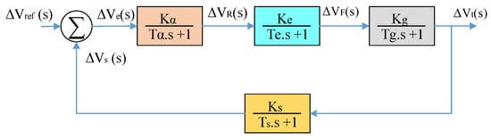
Figure 5.
AVR system block diagram.
There are many different types of excitation systems. In the simplest form, the transfer function of an advanced excitation can be represented by a time constant Te and a gain Ke as Equation (22).
The emf produced by synchronous machines depends on the magnetization curve of the machine and its terminal voltage relays on the load voltage of the generator. The linearized model allows us to write out an equation for the transfer function that describes the relationship between the generator’s terminal voltage and its field voltage with the gain 𝐾g and the time constant Tg as follows:
A voltage transformer is used for sensing the voltage before a rectifier bridge converts it. The sensor is represented by a basic first-order transfer function, which is in the form of Equation (24):
Finally, the closed-loop transfer function that relates the terminal voltage Vt to the reference voltage Vref is expressed as Equation (25):
For the step input ΔVref = 1/s, using the finite value theorem, the steady response is equal to:
3. Design of the Integrated LFC–AVR Based on the FOPI–PIDD2 Controller
To optimally adjust the parameters of the FOPI–PIDD2 controller, the DO algorithm is used. Figure 6 shows the overview of the combined LFC–AVR model along with the coupling coefficients between the two loops under the parameters K1 to K6. Since there may be a mutual connection between these two loops in some cases, when modelling the power system, it needs to be taken into consideration. The real power is determined by the AVR loop, which also regulates the emf (E) that is created. Since frequency is a function of this real power, all adjustments made to the AVR loop need to be monitored by the LFC loop. The change in the output (E) may be attributed to two factors: the first is a change in the field voltage (VF) and the second is the change in the relative position of the rotor or the angle of the rotor (Δδ), as indicated by Equation (27).
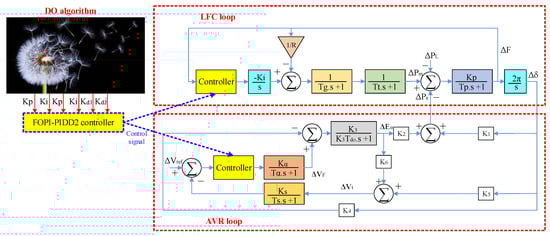
Figure 6.
The combined LFC–AVR model with the proposed controller.
The terminal voltage Vt consists of two components: the voltage Vq on the q axis, which increases with the increase of E, and the voltage Vd on the d axis, which increases with the increase of δ. This relationship is shown by Equation (28).
Up to this part, you have familiarized yourself with the functional structure of LFC–AVR and how to calculate the values of quantities including voltage and frequency changes. Next, the FOPI–PIDD2 controller structure and how to optimally set its parameters will be presented.
3.1. Design of the Proposed FOPI–PIDD2 Controller
The PID controller has been the most well-known and widely used feedback mechanism and has been widely used in the control of various industrial processes. The transfer function C(s) of the PID controller can be defined as Equation (30).
where Kp, Ki, and Kd are proportional, integral, and derivative coefficients, respectively. Thus, the output of the controller will be in the form of Equation (31).
The purpose of designing a PID controller for a system is to determine the Kp, Ki, and Kd coefficients. Depending on the application, the desired output performance of the system can be expressed in different ways. In this section, four important characteristics of the response time of a system are used and the criterion of the system’s output desirability will be defined by them. These features are rise time, settling time, max overshoot, and integral absolute error (IAE). In the following, a brief definition of each of these features is given, and based on them, the optimality criterion of the output response is defined.
Rise time is the time during which the response of the system reaches 90% of its final value from 10%. The rise time is shown in Figure 7. Settling time refers to the time after which the response time of the system remains within 2% of its final response. Max overshoot is defined as the difference between two responses yss and ymax. ymax and yss show the maximum value of the response and its final limit, respectively. Thus, max overshoot is obtained through Equation (32):
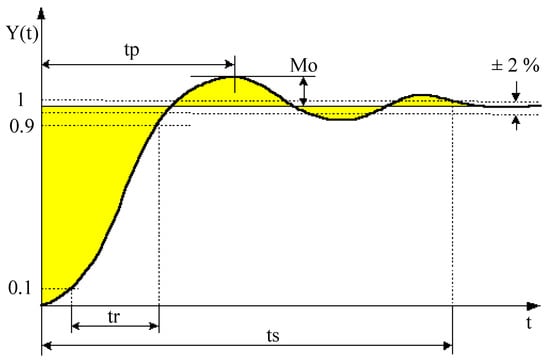
Figure 7.
Rise time (tr), settling time (ts), maximum overshoot (Mo), and the IAE.
The integral of the absolute value of the error is defined through Equation (33).
Due to the implementation of discrete time, in the calculation of this integral, its upper limit up to a certain limit (usually up to three times the settling time) is considered to give an acceptable solution for this integral. The integral absolute error is shown in Figure 7.
The structure of integer order PID controllers can be expanded as a family of fractional controllers. These structures with the transfer function H(s) are as follows:
Integer order PID (IOPID) controller:
Fractional-order proportional-integral (FOPI) controller:
FO(PI) controller:
FO(PD) controller:
FO(PID) controller:
FOPID or PIλDμ controller:
Figure 8a shows that the designer is only limited to the design of four types of controllers P, PI, PD, and PID, while according to Figure 8b, by changing the amount of integration (λ) and the amount of derivation (μ). Between zero and one, in addition to integer controllers, PIλDμ fractional controllers can be designed.
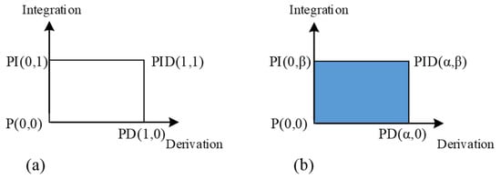
Figure 8.
Integer and fractional order controllers: (a) without changing λ and μ variables and (b) with changing λ and μ variables.
Although integer order PID controllers are commonly utilized in the industry, these regulators do not have the necessary efficiency, especially for high-order systems and fractional systems, so today the use of fractional controllers in the industry is a very new field of research. One of these conventional controllers used for AVR and LFC systems is the FOPI controller. In reference [37], the FOPI controller was used only for the AVR system, and in reference [38], the FOPI controller is used in the LFC system, and its feature is a quick response to the fluctuations made in the system. The disadvantage of these controllers is their inability to improve the phase margin, and the accuracy of the steady state of the system. PIDD2 controller is usually used to solve this problem. The disadvantage of PID controllers is the effect of noise on it and their sensitivity to error changes and not to their value. That is, if the error has a fixed value and does not change, the controller will not react to it. Therefore, to solve these two problems, two D-factors equipped with special filters for noise removal are usually used. The act of derivation is suitable for systems with a large time constant because usually error changes are a prelude to its increase, and the derivative controller provides the necessary preparation for correcting future errors. Since in this article the aim is to enhance the stability of the voltage and frequency loops of an integrated hybrid multi-area power system, the features of both FOPI and PIDD2 controllers have been used and a FOPI–PIDD2 regulator as a secondary controller is suggested. Finally, the configuration of the presented controller is shown in Figure 9, where KP, KI, Kp, Ki, Kd1, and Kd2 are the coefficients of the proposed controller optimized by the DO algorithm, and N1, N2 are the noise filter coefficients to improve the performance of the derivative.
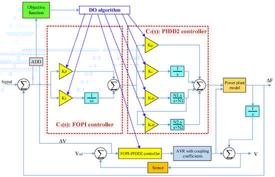
Figure 9.
Structure of the proposed FOPI–PIDD2 controller.
According to Figure 9, the transfer function H(s) of the presented controller may be defined using Equation (40):
where in [39,40],
Finally, the optimal setting of KP, KI, Kp, Ki, Kd1, and Kd2 coefficients in the FOPI–PIDD2 controller is performed using the DO algorithm in such a way that the objective function of Equation (42) is minimized.
Therefore, in this article, the goal is to minimize ITSE with the DO algorithm in such a way that the optimum coefficients of the presented controller are obtained and finally its results can be compared with other algorithms in terms of maximum overshoot (MO), maximum undershoot (MU), settling time (ST), and rise time (RT).
3.2. Improved DO Algorithm for Optimization of the Proposed Controller
In reference [36], a DO algorithm based on the behavior of the dandelion plant is presented to solve optimization problems. In our article, by adding changes in the structure of the algorithm, in addition to improving the DO algorithm, it is used to fine-tune the gains of the FOPI–PIDD2 controller. The DO algorithm consists of three stages including the rising stage, descending stage, and landing stage. Similar to any meta-heuristic algorithm, in the DO algorithm, the initial answers are proposed with random solutions. Assuming that the number of dandelion seed populations is equal to n, the same number of random solutions is needed. Figure 10 shows this process. In this section, the structure of the DO algorithm is described first, and then a solution archive is applied to produce a probabilistic model of variables to improve the DO algorithm. Therefore, the initial population of the DO algorithm is defined as Equation (43).
where pop represents the number of population and Dim is the dimensions of the variables. Since the goal is to optimize the coefficients of KP, KI, Kp, Ki, Kd1, and Kd2, Dim is equal to 6. Each candidate solution is randomly obtained through Equation (44).
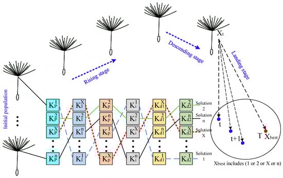
Figure 10.
Generation of initial solutions with the DO algorithm.
After initialization, the rising stage begins. This stage will be different depending on the weather conditions, i.e., when it is windy, the dandelion seeds travel a longer distance, and when it is rainy, they move into their neighborhood. Therefore, two types of searches are performed in the problem space in the rising stage, one is a local search and the other is a general search. In the first type, by considering a lognormal distribution for the wind speed, the position of the dandelion seeds at iteration t+1 can be obtained through Equation (45).
In the second type, on a rainy day, dandelion seeds are moved to the local neighborhood. In this case, the position of the dandelion seeds at iteration t + 1 can be obtained through Equation (46).
After the dandelion seeds have reached a certain distance, it is time for the descending stage. In this part, the movement of dandelion seeds based on Brownian motion (βt) is expressed with a normal distribution, so that it can be obtained from the average position information after the rising stage. Therefore, the new position of the dandelion seeds in this step is calculated through Equation (47).
Finally, in the last stage, the dandelion seeds choose their random position in the landing stage. With more iterations, it is hoped to reach the global optimal solution. At this stage, the global optimal solution can be achieved by sharing Xbest information through search agents to local neighborhoods. Therefore, we will have Equation (48):
So far, you are familiar with the structure of the DO algorithm, which is fully explained in reference [36]. In the following, to implement the DO algorithm in the optimization of the FOPI–PIDD2 controller, we have added a series of changes to it to better evaluate the solutions. Here, we consider a section as a solution archive similar to Figure 11, and the solutions are stored in ascending order of the cost function. The solution archive is used to create new solutions. The importance of each solution in the solution archive can be determined with a weight coefficient. Considering that the first solution in the archive has better performance, it should have the highest weight factor and the last member of this archive should have the least importance. Therefore, any descending function satisfies this requirement according to the position of the solutions. In this research, this weight function for the solution with the xth position is considered as Equation (49):
where k is the size of the solution archive, and the positive parameter q is the selection pressure in the sense that it specifies the weight difference between the solutions. Given the small values of q, the best solutions are strongly preferred and have priority in suggesting new solutions, and the larger q is, the more uniform the probabilities become. According to Equation (49), between the weights assigned to the solutions in the archive, Equation (50) will be:
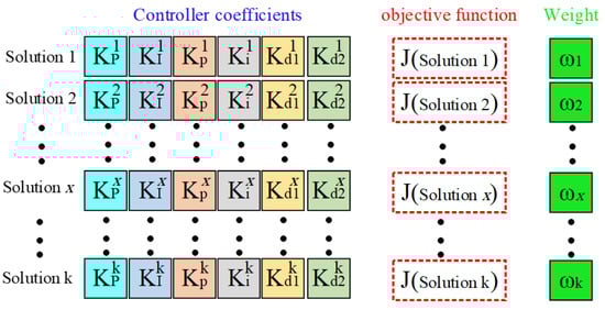
Figure 11.
Solution archive.
The probability of choosing the xth solution is obtained through Equation (51).
Considering that the space of decision variables is continuous, the distribution should be continuous in the search space. This demand will be expressed with the Gaussian kernel, which is a linear combination of Gaussian probability functions. In this way, for the six decision parameters KP, KI, Kp, Ki, Kd1, and Kd2 based on the solution archive, probabilistic description is considered in the form of Equation (52).
Now, to better explain how these Gaussian kernels work, let us assume that the size of the solution archive is equal to six, and KP1, KP2, KP3, KP4, KP5, and KP6 are proposals for the controller’s proportional parameter. Since the search space is a continuous variable, it is necessary to use a continuous distribution centered around these solutions. This demand can be met with the Gaussian density function and its average is equal to the existing solutions. Now, the amount of searching around the neighborhood of the solution or the variance of the Gaussian density function must be determined. A suitable choice for each solution to cover its surrounding space is determined by Equation (53):
These concepts are depicted in Figure 12. According to Equation (53), the variance is proportional to the average distance of the proposed solution from the rest of the solutions in the archive. If the concentration of solutions is high in one area, a small variance will be allocated to that solution, and on the contrary, if the solution is far away from the rest of the solutions, the variance will be a large value to cover all the space where the possible solution was not available.
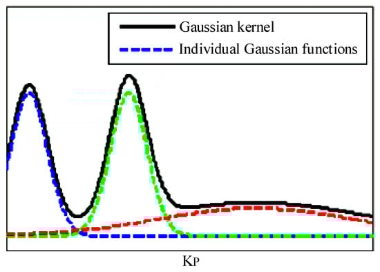
Figure 12.
An example of three Gaussian density functions and Gaussian kernel.
For updating, Gaussian kernels Gl = 1, 2, 3, 4, 5, 6 and roulette cycle are used to produce a new solution as many as the population of dandelion seeds. The sampling process and the use of Gaussian kernel functions can be described as follows: first, six random numbers such as 𝜛1, 𝜛2, 𝜛3, 𝜛4, 𝜛5, 𝜛6 are generated and the first set of solutions will be selected for the six existing decision variables, which apply to the relationships 𝜛1 < 𝑝1, 𝜛2 < 𝑝2, 𝜛3 < 𝑝3, 𝜛4 < 𝑝4, 𝜛5 < 𝑝5, 𝜛6 < 𝑝6. Note that 𝑝1 to 𝑝6 are defined in Equation (51). The new solution using the existing distributions will be in the form of Equation (54).
Finally, the new solutions are merged with the solution archive and the solution archive is updated by selecting k from the best solutions.
3.3. Configuration of the Studied Hybrid Two-Area System
In this research, according to Figure 13, a study is performed on the hybrid dual-area power system. As you can see, area 1 includes thermal units, wind farms, and electric vehicles, and area 2 includes hydraulic units, solar farms, and electric vehicles, which are linked through a tie-line. Here, to evaluate and analyze the system’s dynamic response to voltage and frequency changes, it is necessary to design a small signal block diagram model of the two-area power system based on the transfer function of the network components. According to that presented in Section 2.1 of the article, the thermal unit model comprised of a governor, limiter, and turbine; the hydraulic unit model comprised of a governor, limiter, transient droop compensation, and turbine; and the AVR model consists of an amplifier, exciter, generator, sensor, AVR coupling coefficients, and other components which include solar PV, wind turbine, EV, area swing 1, area swing 2, T-line, frequency bias coefficients, and speed droops, whose complete information is shown in Table 1. Finally, according to the model of the different components of the hybrid dual-area power system in Table 1, the small signal block diagram of the hybrid dual-area power system with the proposed controller is shown in Figure 14.
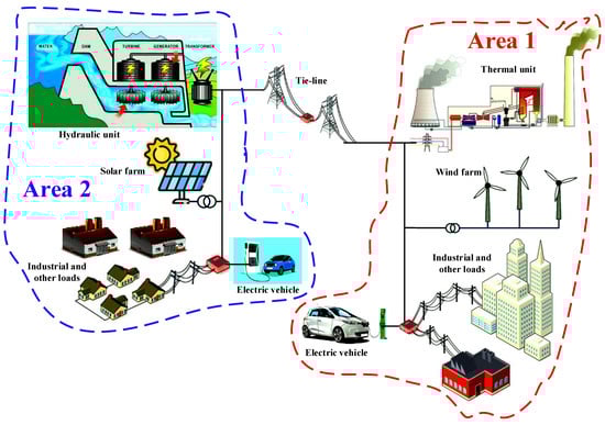
Figure 13.
Hybrid two-area power system under study.

Table 1.
The transfer functions presented in the investigated hybrid power system and their parameters’ values.
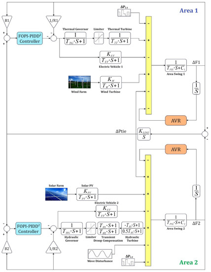
Figure 14.
The investigated hybrid two-area system model with the suggested controller.
4. Simulation Results and Discussion
Herein, the efficiency of the optimized FOPI–PIDD2 controller with the DO algorithm on the power system presented in Figure 13 has been evaluated using simulation in MATLAB software for different conditions. Here, the system parameters are presented in Table 1, considering the existence of hydraulic units, solar farms, and wind farms in the system and the dependence of these units on wave disturbance variation, fluctuation of solar radiation, and wind speed fluctuation in the order of output power changes of these units in Figure 15, Figure 16, Figure 17, Figure 18 and Figure 19 are shown [39].
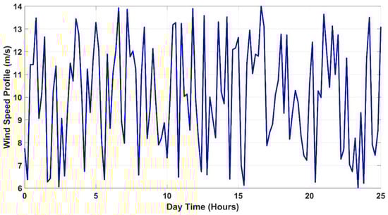
Figure 15.
Wind speed fluctuation.
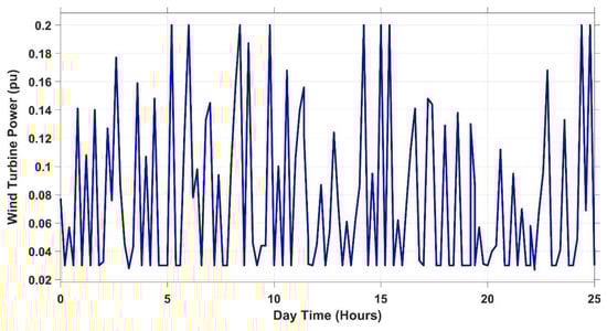
Figure 16.
Wind turbine power variation.
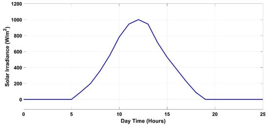
Figure 17.
Fluctuation of solar radiation.
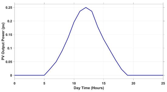
Figure 18.
PV output power fluctuation.
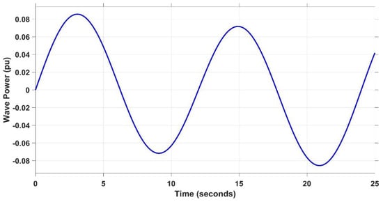
Figure 19.
Wave disturbance variation.
So far, various controllers with different algorithms for voltage and frequency stability have been presented in the articles, and in this article, the performance of the presented regulator has been put in a comparison with some of these methods. Among the factors affecting the performance of the regulator that cause disturbances in the system, we can mention load disturbances, power changes of generation units, transmission time delay, disconnection of electric vehicles, and uncertainty of parameters. In this article, the performance of the recommended regulator has been tested under various circumstances, and its results have been compared to those of alternative techniques. Consequently, the following cases have been examined:
- Scenario 1: Step load variation (SLV) impact.
- Scenario 2: Random load variation (RLV) and time-varying desired voltage (TVDV) impact.
- Scenario 3: Solar irradiance variation impact.
- Scenario 4: Wind speed variation impact.
- Scenario 5: Wave variation impact.
- Scenario 6: Consideration of all RESs as well as TVDV.
- Scenario 7: Communication time delay (CTD) impact.
- Scenario 8: Disconnection of electric vehicles (EVs) impact.
- Scenario 9: System parameter variation impact.
4.1. Scenario 1: Step Load Variation (SLV) Impact
Considering that the load change in the power system is generally performed by disconnecting or connecting constant values, in the voltage–frequency study of the system, the step input is used to model the load changes. To analyze the response of the system to step load change, in scenario 1, we first consider a situation where 5% step load disturbance occurs in area 2. In reference [39] of wild horse optimizer (WHO) to optimize the fuzzy fractional-order PI and TID controllers and in reference [40] of the gradient-based optimizer (GBO) to optimize the fuzzy–PIDD2 controller and in reference [41] artificial ecosystem-based optimization (AEO) has been used to optimize the PID controller, and here these algorithms have been used to optimize the proposed FOPI–PIDD2 controller and its results have been compared with the DO algorithm. As seen in Figure 20, the process of convergence and reduction of the ITSE function is shown in 200 iterations for the mentioned algorithms, and the proposed DO algorithm has the lowest amount of error. In this scenario, thermal, hydraulic, and electric vehicle units are connected to the system.
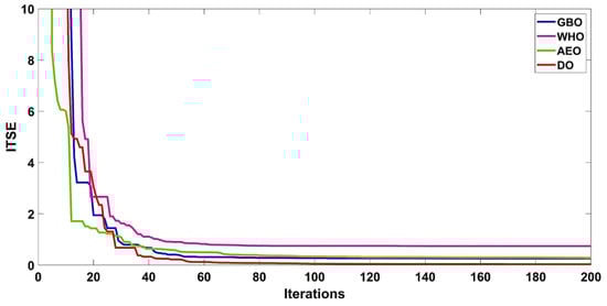
Figure 20.
Convergence characteristics of all investigated algorithms.
In reference [42], a PD–PIDD2 controller and reference [43] a TD–TI controller are proposed for system frequency stability, where the performance of these controllers is compared with the proposed FOPI–PIDD2 controller, such that these three controllers are optimized through the DO algorithm. As you can see in Figure 21, the performance of the presented regulator has been compared with two other controllers, which are shown in the order of the voltage and frequency fluctuations of areas 1 and 2 and the power of the tie line. As shown in Figure 21a,b, the results show the superiority of the proposed controller from the point of voltage control. The terminal voltages are settled quickly with lower settling and rise times. Furthermore, Figure 21c–e show the efficiency of the proposed FOPI–PIDD2 controller, from the point of frequency and tie-line power control, in the faster and smoother damping of oscillations due to strong reduction of overshoot, reduction of nearly one-sixth of the settling time, and reduction of all values of the error criteria compared to the PD–PIDD2 and TD–TI controllers and as a result, improving the dynamic stability of the power system. Table 2 and Table 3, respectively, show the results related to the optimal parameters of controllers and dynamic specifications under the influence of different criteria.
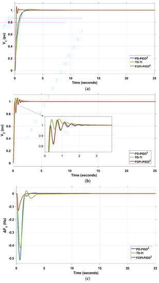
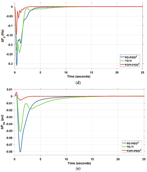
Figure 21.
Comparison of PD–PIDD2, TD–TI, and FOPI–PIDD2 optimized by DO algorithm for scenario 1: (a) V1, (b) V2, (c) ΔF1, (d) ΔF2, and (e) ΔPtie.
Table 2.
Optimal parameters of the three controllers for scenario 1.
Table 3.
Dynamic specifications of the investigated system using different controllers under scenario 1 impact.
4.2. Scenario 2: Random Load Variation (RLV) and Time-Varying Desired Voltage (TVDV) Impact
In this scenario, the simultaneous effect of random load variation and time-varying desired voltage is applied to the studied system to evaluate the performance of the regulator. Thus, according to Figure 22, a random load variation in area 2 and time-varying desired voltage for both areas are considered according to Figure 23. Here, the same optimal parameters obtained from scenario 1 according to Table 2 are used for the controller. Figure 24 shows the performance results of the suggested controller. In this scenario, thermal, hydraulic, and electric vehicle units are connected to the system.
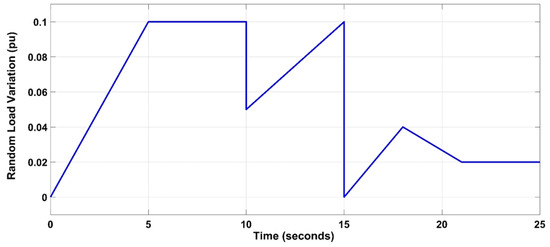
Figure 22.
Random load variation.
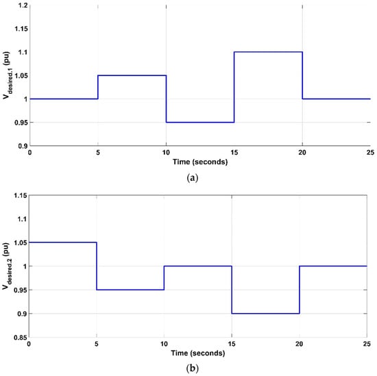
Figure 23.
The time-varying desired voltage (a) in area 1 and (b) in area 2.
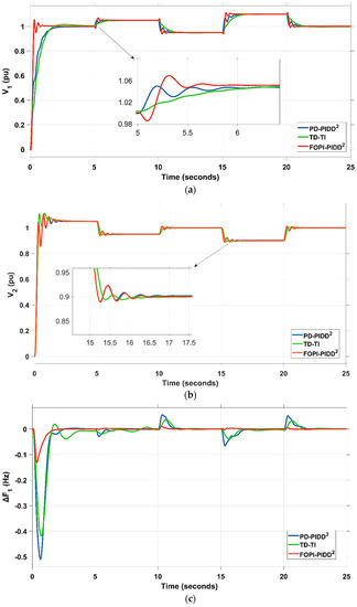
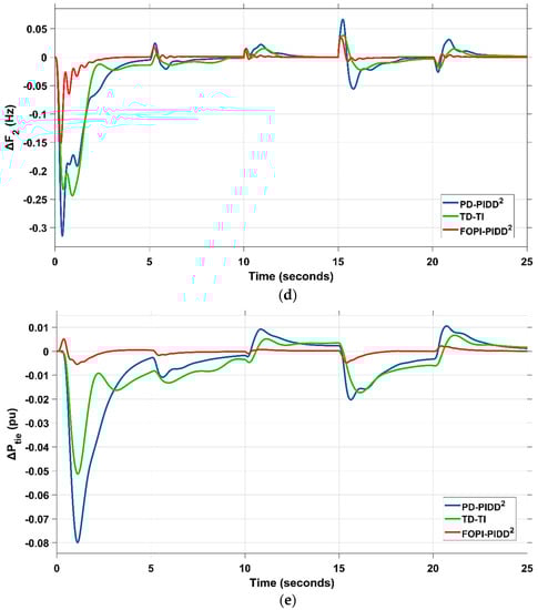
Figure 24.
Comparison of PD–PIDD2, TD–TI, and FOPI–PIDD2 optimized by DO algorithm for scenario 2: (a) V1, (b) V2, (c) ΔF1, (d) ΔF2, and (e) ΔPtie.
As you can see in Figure 24, the proposed controller has the loss of the least ripple of fluctuations and has obtained the lowest value of the objective function defined in Equation (42), the results of which are shown in Table 4. According to Table 4, the proposed controller has been able to obtain a value of the objective function that is approximately 2.95 times lower than the TD–TI controller and 2.47 times lower than the PD–PIDD2 controller. As it is clear from the objective function, by minimizing it, the proposed controller has been able to perform the best in terms of fluctuations in voltage, frequency, and power tie.
Table 4.
Dynamic specifications of the investigated system represented as ITSE value using different controllers under scenario 2 impact.
4.3. Scenario 3: Solar Irradiance Variation Impact
In this scenario, the effect of the PV unit on the proposed controller in area 2 of the power system is evaluated according to Figure 18. Figure 25 and Table 5 show the results of this case. The presented controller has the ability to obtain a value of the objective function that is approximately 28.9 times lower than the TD–TI controller and 6.1 times lower than the PD–PIDD2 controller. Therefore, the presence of the PV unit in the system had a severe impact on the performance of the two TD–TT and PD–PIDD2 controllers, but the proposed controller had a better performance, which was 2.5 times less than scenario 2. In this scenario, thermal, hydraulic, solar farm, and electric vehicle units are connected to the system.
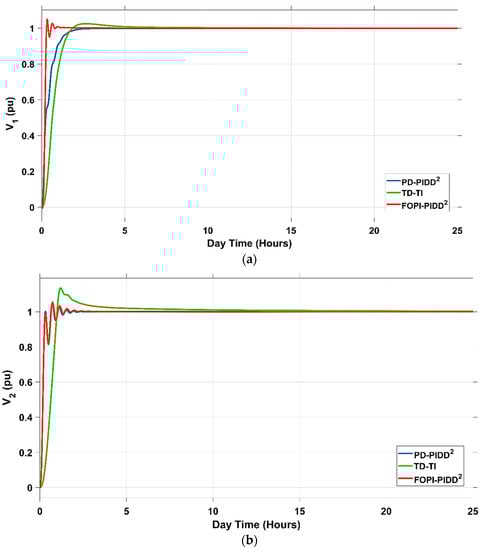
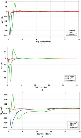
Figure 25.
Comparison of PD–PIDD2, TD–TI, and FOPI–PIDD2 optimized by DO algorithm for scenario 3: (a) V1, (b) V2, (c) ΔF1, (d) ΔF2, and (e) ΔPtie.
Table 5.
Dynamic specifications of the investigated system represented as ITSE value using different controllers under scenario 3 impact.
4.4. Scenario 4: Wind Speed Variation Impact
Herein, the impact of the wind farm unit on the proposed controller in area 1 of the power system is evaluated according to Figure 16, whose results are shown in Figure 26 and Table 6. In this scenario, thermal, hydraulic, wind farm, and electric vehicle units are connected to the system. The presented controller has the ability to obtain a value of the objective function that is approximately 6.98 times lower than the TD–TI controller and 6.45 times lower than the PD–PIDD2 controller. As you can see in Figure 26, the wind farm had a great effect on the two controllers TD–TT and PD–PIDD2 in such a way that it caused severe fluctuations, which were relatively less in the proposed controller.
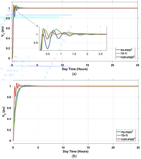
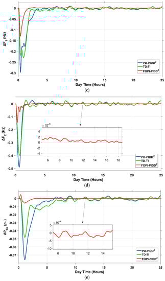
Figure 26.
Comparison of PD–PIDD2, TD–TI, and FOPI–PIDD2 optimized by DO algorithm for scenario 4: (a) V1, (b) V2, (c) ΔF1, (d) ΔF2, and (e) ΔPtie.
Table 6.
Dynamic specifications of the investigated system represented as ITSE value using different controllers under scenario 4 impact.
4.5. Scenario 5: Wave Variation Impact
In this scenario, the investigated system is exposed to wave energy fluctuations in area 2, and an analysis of the system’s performance is presented. In a manner analogous to that which was tested in the earlier scenarios, the effectiveness of the suggested combination of FOPI and PIDD2 as tuned by the DO algorithm is evaluated in terms of its ability to minimize the deviations in voltage and frequency and to keep the system stable under the current circumstances. In this scenario, thermal, hydraulic, and electric vehicle units are connected to the system. Table 7 provides a summary of the ITSE values calculated by various controllers while taking into account the influence of varying wave energies. By utilizing the suggested FOPI–PIDD2 combination, one may attain the ITSE value that is the lowest possible. Figure 27 also illustrates the dynamics of the system when subjected to this particular situation. It is clear that the combination of FOPI and PIDD2 suggested here offers superior oscillation damping compared to the other controllers that were tested for comparison. This demonstrates that the combination that was suggested was successful in dealing with extreme variations and disruptions that were occurring.
Table 7.
Dynamic specifications of the investigated system represented as ITSE value using different controllers under scenario 5 impact.
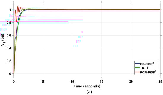
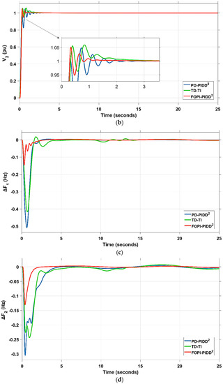
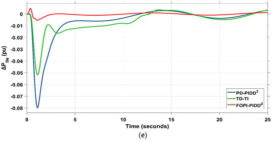
Figure 27.
Assessment of PD–PIDD2, TD–TI, and FOPI–PIDD2 optimized by DO algorithm for scenario 5: (a) V1, (b) V2, (c) ΔF1, (d) ΔF2, and (e) ΔPtie.
4.6. Scenario 6: Consideration of all RESs as Well as TVDV
In this scenario, the impact of the previous scenarios is considered simultaneously, so that all units including hydraulic, thermal, solar farm, wind farm, and electric vehicles are present in the system. In this particular scenario, area 2 of the power system is impacted by variations in solar irradiance as well as wave energy fluctuations, whereas area 1 is influenced by variations in the wind speed, and both areas are subjected to the time-varying desired voltages that are previously mentioned in scenario 2. This seeks to demonstrate the effectiveness of the suggested DO-based FOPI–PIDD2 combination over existing controllers in maintaining system stability under harsh conditions, whose results are shown in Figure 28 and Table 8. The presented controller has the ability to obtain a value of the objective function that is approximately 2.99 times lower than the TD–TI controller and 2.28 times lower than the PD–PIDD2 controller.
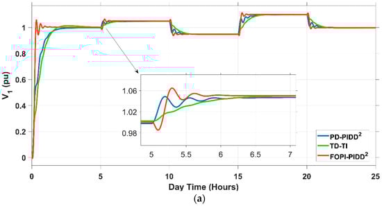
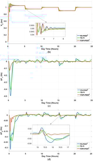
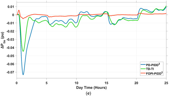
Figure 28.
Comparison of PD–PIDD2, TD-–TI, and FOPI–PIDD2 optimized by DO algorithm for scenario 6: (a) V1, (b) V2, (c) ΔF1, (d) ΔF2, and (e) ΔPtie.
Table 8.
Dynamic specifications of the investigated system represented as ITSE value using different controllers under scenario 6 impact.
4.7. Scenario 7: Communication Time Delay (CTD) Impact
In this situation, a CTD of 0.05 s is deployed to the controllers’ output. In addition, 3% and 5% step load perturbations are inserted to area 1 and area 2, respectively. Table 9 outlines the various PD–PIDD2, TD–TI, and FOPI–PIDD2 controller settings. The system’s dynamic performance, in this situation, is summarized in Table 10. In addition, Figure 29 presents the dynamics of the system under this scenario. In this scenario, thermal, hydraulic, and electric vehicle units are connected to the system. The presented controller has the ability to obtain a value of the objective function that is approximately 4.94 times lower than the TD–TI controller and 12.61 times lower than the PD–PIDD2 controller.
Table 9.
Optimal parameters of the three controllers for scenario 7.
Table 10.
Dynamic specifications of the investigated system using different controllers under scenario 7 impact.
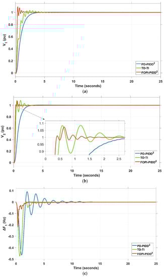
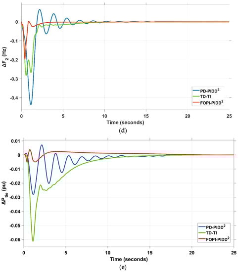
Figure 29.
Comparison of PD–PIDD2, TD–TI, and FOPI–PIDD2 optimized by DO algorithm for scenario 7: (a) V1, (b) V2, (c) ΔF1, (d) ΔF2, and (e) ΔPtie.
4.8. Scenario 8: Integration of Electric Vehicles (EVs) Impact
Here, the suggested FOPI–PIDD2 combination is used to assess the impact of an integration of EVs in the two regions comprising the system under investigation. To decouple load requirements and system generations, electric vehicle battery storage is utilized. This is especially helpful when there is a deficit in the amount of power generated in each respective region. Figure 30 shows the dynamic response of V1, V2, ΔF1, ΔF2, and ΔPtie using the proposed controller when EVs are integrated into the system. The ITSE value is shown in Table 11 both with and without the inclusion of EVs. When electric vehicles are linked to the system, the ITSE may be made to reach its minimum value, which is something that can be noticed.
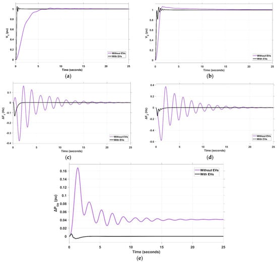
Figure 30.
System dynamics for scenario 8 when using FOPI–PIDD2 controller: (a) V1, (b) V2, (c) ΔF1, (d) ΔF2, and (e) ΔPtie.
Table 11.
Dynamic specifications of the investigated system represented as ITSE value using the proposed controller under scenario 8 impact.
4.9. Scenario 9: System Parameter Variation Impact
The objective of this scenario is to put the suggested FOPI–PIDD2 controller’s resilience to the test by presenting the sensitivity analysis for the variations in system parameters. Alterations of are made to a few system settings such as TH1, THG, KEV, TEV, KLINE, B1, and B2. Table 12 provides a summary of the outcomes of the sensitivity analysis accomplished by altering the abovementioned system parameters.
Table 12.
Dynamic response specifications under the effect of variation in system parameters.
5. Conclusions
To improve the voltage and frequency responses of a dual-area linked power system, a novel combined FOPI–PIDD2 regulator is suggested. The hybrid system incorporates RESs such as wind and solar photovoltaics (PV), along with traditional energy sources such as non-reheat thermal unit and hydroelectric unit. Moreover, electric vehicles (EVs) are deployed in both regions. An up-to-date metaheuristic optimization technique called dandelion optimizer (DO) was used to determine the suggested controller’s ideal settings. In comparison to the GBO, WHO, and AEO algorithms, the DO algorithm offers faster convergence and better accuracy. Step load variation (SLV), random load variation (RLV), wind speed variation, solar irradiance alteration, and wave energy fluctuations are only some of the uncertainties that have been applied to assess the resilience of the suggested controller. The outcomes reveal that the objective function in terms of the ITSE index was considerably enhanced using the suggested FOPI–PIDD2 controller by 86% compared to the other recent controllers (TD–TI, PD–PIDD2). In addition, EVs contribute to greater system stability. Even with a 25% variation in some system parameters, the DO-based FOPI–PIDD2 controller maintains a high degree of precision.
Author Contributions
Conceptualization, M.A.; validation, M.R.; investigation, K.M.A.; writing—original draft preparation, M.D.; supervision, H.K.; project administration, M.S.; funding acquisition, E.E. All authors have read and agreed to the published version of the manuscript.
Funding
This research received no external funding.
Institutional Review Board Statement
Not applicable.
Informed Consent Statement
Not applicable.
Data Availability Statement
The data sources employed for analysis are presented in the text.
Acknowledgments
This work was supported by the Researchers Supporting Project number (RSP2023R467), King Saud University, Riyadh, Saudi Arabia.
Conflicts of Interest
The authors declare no conflict of interest.
References
- Kundur, P.S.; Om, P.M. Power System Stability and Control; McGraw-Hill Education: New York, NY, USA, 2022. [Google Scholar]
- Shouran, M.; Anayi, F.; Packianather, M.; Habil, M. Load Frequency Control Based on the Bees Algorithm for the Great Britain Power System. Designs 2021, 5, 50. [Google Scholar] [CrossRef]
- Kalyan, C.N.S.; Rao, G.S. Frequency and voltage stabilisation in combined load frequency control and automatic voltage regulation of multiarea system with hybrid generation utilities by AC/DC links. Int. J. Sustain. Energy 2020, 39, 1009–1029. [Google Scholar] [CrossRef]
- Grover, H.; Verma, A.; Bhatti, T. Load frequency control & automatic voltage regulation for a single area power system. In Proceedings of the 2020 IEEE 9th Power India International Conference (PIICON), Sonepat, India, 28 February–1 March 2020; pp. 1–5. [Google Scholar]
- Dashtdar, M.; Flah, A.; El-Bayeh, C.Z.; Tostado-Véliz, M.; Al Durra, A.; Aleem, S.H.A.; Ali, Z.M. Frequency control of the islanded microgrid based on optimised model predictive control by PSO. IET Renew. Power Gener. 2022, 16, 2088–2100. [Google Scholar] [CrossRef]
- Abuagreb, M.; Ajao, B.; Herbert, H.; Johnson, B.K. Evaluation of virtual synchronous generator compared to synchronous generator. In Proceedings of the 2020 IEEE Power & Energy Society Innovative Smart Grid Technologies Conference (ISGT), Washington, DC, USA, 17 –20 February 2020; pp. 1–5. [Google Scholar]
- Abuagreb, M.; Allehyani, M.F.; Johnson, B.K. Overview of Virtual Synchronous Generators: Existing Projects, Challenges, and Future Trends. Electronics 2022, 11, 2843. [Google Scholar] [CrossRef]
- Shouran, M.; Anayi, F.; Packianather, M. The Bees Algorithm Tuned Sliding Mode Control for Load Frequency Control in Two-Area Power System. Energies 2021, 14, 5701. [Google Scholar] [CrossRef]
- Ismail, M.M.; Bendary, A.F. Load Frequency Control for Multi Area Smart Grid based on Advanced Control Techniques. Alex. Eng. J. 2018, 57, 4021–4032. [Google Scholar] [CrossRef]
- Dashtdar, M.; Flah, A.; Hosseinimoghadam, S.M.S.; Reddy, C.R.; Kotb, H.; AboRas, K.M.; Bortoni, E.C. Improving the Power Quality of Island Microgrid with Voltage and Frequency Control Based on a Hybrid Genetic Algorithm and PSO. IEEE Access 2022, 10, 105352–105365. [Google Scholar] [CrossRef]
- Abubakr, H.; Vasquez, J.C.; Mohamed, T.H.; Guerrero, J.M. The concept of direct adaptive control for improving voltage and frequency regulation loops in several power system applications. Int. J. Electr. Power Energy Syst. 2022, 140, 108068. [Google Scholar] [CrossRef]
- Mojumder, H.M.R.; Roy, N.K. PID, LQR, and LQG Controllers to Maintain the Stability of an AVR System at Varied Model Parameters. In Proceedings of the 2021 5th International Conference on Electrical Engineering and Information & Communication Technology (ICEEICT), Dhaka, Bangladesh, 18–20 November 2021; pp. 1–6. [Google Scholar]
- Lai, H.B.; Tran, A.T.; Huynh, V.; Amaefule, E.N.; Tran, P.T.; Phan, V.D. Optimal linear quadratic Gaussian control based frequency regulation with communication delays in power system. Int. J. Electr. Comput. Eng. 2022, 12, 157–165. [Google Scholar] [CrossRef]
- Bhutto, D.K.; Ansari, J.; Zameer, H. Implementation of AI Based Power Stabilizer Using Fuzzy and Multilayer Perceptron In MatLab. In Proceedings of the 2020 3rd International Conference on Computing, Mathematics and Engineering Technologies (iCoMET), Sukkur, Pakistan, 29–30 January 2020; pp. 1–8. [Google Scholar]
- Hosseinimoghadam, S.M.S.; Dashtdar, M.; Dashtdar, M.; Roghanian, H. Security control of islanded micro-grid based on adaptive neuro-fuzzy inference system. Sci. Bull. Ser. C Electr. Eng. Comput. Sci. 2020, 1, 189–204. [Google Scholar]
- Modabbernia, M.; Alizadeh, B.; Sahab, A.; Moghaddam, M.M. Designing the Robust Fuzzy PI and Fuzzy Type-2 PI Controllers by Metaheuristic Optimizing Algorithms for AVR System. IETE J. Res. 2020, 68, 3540–3554. [Google Scholar] [CrossRef]
- Bhutto, A.A.; Chachar, F.A.; Hussain, M.; Bhutto, D.K.; Bakhsh, S.E. Implementation of probabilistic neural network (PNN) based automatic voltage regulator (AVR) for excitation control system in Matlab. In Proceedings of the 2019 2nd International Conference on Computing, Mathematics and Engineering Technologies (iCoMET), Sukkur, Pakistan, 30–31 January 2019; pp. 1–5. [Google Scholar]
- Nahas, N.; Abouheaf, M.; Darghouth, M.N.; Sharaf, A. A multi-objective AVR-LFC optimization scheme for multi-area power systems. Electr. Power Syst. Res. 2021, 200, 107467. [Google Scholar] [CrossRef]
- Kalyan, C.N.S.; Goud, B.S.; Reddy, C.R.; Bajaj, M.; Sharma, N.K.; Alhelou, H.H.; Siano, P.; Kamel, S. Comparative Performance Assessment of Different Energy Storage Devices in Combined LFC and AVR Analysis of Multi-Area Power System. Energies 2022, 15, 629. [Google Scholar] [CrossRef]
- Aguila-Camacho; Norelys; García-Bustos, J.E.; Castillo-López, E.I. Switched Fractional Order Model Reference Adaptive Control for an Automatic Voltage Regulator. In International Design Engineering Technical Conferences and Computers and Information in Engineering Conference; American Society of Mechanical Engineers: New York City, NY, USA, 2021; Volume 85437, p. V007T07A017. [Google Scholar]
- Safiullah, S.; Rahman, A.; Ahmad Lone, S. Optimal control of electrical vehicle incorporated hybrid power system with second order fractional-active disturbance rejection controller. Optim. Control. Appl. Methods 2021. [Google Scholar] [CrossRef]
- Aljaifi, T.; Bawazir, A.; Abdellatif, A.; Pauline, O.; Yee, L.C.; Abdullah, H. Applying genetic algorithm to optimize the PID controller parameters for an effective automatic voltage regulator. Commun. Comput. Appl. Math. 2019, 1, 10–15. [Google Scholar]
- Yegireddy, N.K.; Panda, S.; Papinaidu, T.; Yadav, K.P.K. Multi-objective non dominated sorting genetic algorithm-II optimized PID controller for automatic voltage regulator systems. J. Intell. Fuzzy Syst. 2018, 35, 4971–4975. [Google Scholar] [CrossRef]
- Guha, D.; Roy, P.K.; Banerjee, S.; Padmanaban, S.; Blaabjerg, F.; Chittathuru, D. Small-Signal Stability Analysis of Hybrid Power System with Quasi-Oppositional Sine Cosine Algorithm Optimized Fractional Order PID Controller. IEEE Access 2020, 8, 155971–155986. [Google Scholar] [CrossRef]
- Kamel, S.; Elkasem, A.H.A.; Korashy, A.; Ahmed, M.H. Sine Cosine Algorithm for Load Frequency Control Design of Two Area Interconnected Power System with DFIG Based Wind Turbine. In Proceedings of the 2019 International Conference on Computer, Control, Electrical, and Electronics Engineering (ICCCEEE), Khartoum, Sudan, 21–23 September 2019. [Google Scholar]
- Ghosh, A.; Ray, A.K.; Nurujjaman; Jamshidi, M. Voltage and frequency control in conventional and PV integrated power systems by a particle swarm optimized Ziegler–Nichols based PID controller. SN Appl. Sci. 2021, 3, 314. [Google Scholar] [CrossRef]
- Ebrahim, M.A.; Ali, A.M.; Hassan, M.M. Frequency and voltage control of multi area power system via novel particle swarm optimization techniques. Int. J. Comput. Res. 2017, 24, 427–474. [Google Scholar]
- Mokeddem, D.; Mirjalili, S. Improved Whale Optimization Algorithm applied to design PID plus second-order derivative controller for automatic voltage regulator system. J. Chin. Inst. Eng. 2020, 43, 541–552. [Google Scholar] [CrossRef]
- Taher, S.A.; Fini, M.H.; Aliabadi, S.F. Fractional order PID controller design for LFC in electric power systems using imperialist competitive algorithm. Ain Shams Eng. J. 2014, 5, 121–135. [Google Scholar] [CrossRef]
- Mahmoud, E. Design of neural network predictive controller based on imperialist competitive algorithm for automatic voltage regulator. Neural Comput. Appl. 2019, 31, 5017–5027. [Google Scholar]
- Chatterjee, S.; Mukherjee, V. PID controller for automatic voltage regulator using teaching–learning based optimization technique. Int. J. Electr. Power Energy Syst. 2016, 77, 418–429. [Google Scholar] [CrossRef]
- Yeboah, S.J. Gravitational Search Algorithm Based Automatic Load Frequency Control for Multi-Area Interconnected Power System. Turk. J. Comput. Math. Educ. (TURCOMAT) 2021, 12, 4548–4568. [Google Scholar]
- Alhelou, H.H.; Hamedani-Golshan, M.E.; Zamani, R.; Heydarian-Forushani, E.; Siano, P. Challenges and opportunities of load frequency control in conventional, modern and future smart power systems: A comprehensive review. Energies 2018, 11, 2497. [Google Scholar] [CrossRef]
- Ali, T.; Malik, S.A.; Daraz, A.; Aslam, S.; Alkhalifah, T. Dandelion Optimizer-Based Combined Automatic Voltage Regulation and Load Frequency Control in a Multi-Area, Multi-Source Interconnected Power System with Nonlinearities. Energies 2022, 15, 8499. [Google Scholar] [CrossRef]
- Ali, M.H.; Soliman, A.M.A.; Ahmed, M.F.; Adel, A.H. Optimization of Reactive Power Dispatch Considering DG Units Uncertainty By Dandelion Optimizer Algorithm. Int. J. Renew. Energy Res. (IJRER) 2022, 12, 1805–1818. [Google Scholar] [CrossRef]
- Zhao, S.; Zhang, T.; Ma, S.; Chen, M. Dandelion Optimizer: A nature-inspired metaheuristic algorithm for engineering applications. Eng. Appl. Artif. Intell. 2022, 114, 105075. [Google Scholar] [CrossRef]
- Padiachy, V.; Mehta, U.; Azid, S.; Prasad, S.; Kumar, R. Two degree of freedom fractional PI scheme for automatic voltage regulation. Eng. Sci. Technol. Int. J. 2021, 30, 101046. [Google Scholar] [CrossRef]
- Pathak, P.K.; Yadav, A.K.; Padmanaban, S.; Kamwa, I. Fractional Cascade LFC for Distributed Energy Sources via Advanced Optimization Technique Under High Renewable Shares. IEEE Access 2022, 10, 92828–92842. [Google Scholar] [CrossRef]
- Ali, M.; Kotb, H.; AboRas, M.K.; Abbasy, H.N. Frequency regulation of hybrid multi-area power system using wild horse optimizer based new combined Fuzzy Fractional-Order PI and TID controllers. Alex. Eng. J. 2022, 61, 12187–12210. [Google Scholar] [CrossRef]
- Hossam-Eldin, A.A.; Negm, E.; Ragab, M.; AboRas, K.M. A maiden robust FPIDD2 regulator for frequency-voltage enhancement in a hybrid interconnected power system using Gradient-Based Optimizer. Alex. Eng. J. 2022, 65, 103–118. [Google Scholar] [CrossRef]
- Ćalasan, M.; Micev, M.; Djurovic, Ž.; Mageed, H.M.A. Artificial ecosystem-based optimization for optimal tuning of robust PID controllers in AVR systems with limited value of excitation voltage. Int. J. Electr. Eng. Educ. 2020, 0020720920940605. [Google Scholar] [CrossRef]
- Khudhair, M.; Ragab, M.; AboRas, K.M.; Abbasy, N.H. Robust Control of Frequency Variations for a Multi-Area Power System in Smart Grid Using a Newly Wild Horse Optimized Combination of PIDD2 and PD Controllers. Sustainability 2022, 14, 8223. [Google Scholar] [CrossRef]
- Elkasem, A.H.A.; Khamies, M.; Hassan, M.H.; Agwa, A.M.; Kamel, S. Optimal Design of TD-TI Controller for LFC Considering Renewables Penetration by an Improved Chaos Game Optimizer. Fractal Fract. 2022, 6, 220. [Google Scholar] [CrossRef]


Disclaimer/Publisher’s Note: The statements, opinions and data contained in all publications are solely those of the individual author(s) and contributor(s) and not of MDPI and/or the editor(s). MDPI and/or the editor(s) disclaim responsibility for any injury to people or property resulting from any ideas, methods, instructions or products referred to in the content. |
© 2023 by the authors. Licensee MDPI, Basel, Switzerland. This article is an open access article distributed under the terms and conditions of the Creative Commons Attribution (CC BY) license (https://creativecommons.org/licenses/by/4.0/).