Neimark–Sacker Bifurcation of a Discrete-Time Predator–Prey Model with Prey Refuge Effect

Abstract

In this paper, we deduce a predator–prey model with discrete time in the interior of ${\mathbb{R}}_{+}^2$ using a new discrete method to study its local dynamics and Neimark–Sacker bifurcation. Compared with continuous models, discrete ones have many unique properties that help to understand the changing patterns of biological populations from a completely new perspective. The existence and stability of the three equilibria are analyzed, and the formation conditions of Neimark–Sacker bifurcation around the unique positive equilibrium point are established using the center manifold theorem and bifurcation theory. An attracting closed invariant curve appears, which corresponds to the periodic oscillations between predators and prey over a long period of time. Finally, some numerical simulations and their biological meanings are given to reveal the complex dynamical behavior.

1. Introduction

Theoretical ecology aims to give reasonable explanations for the interactions among biological populations in nature with the help of dynamical models to predict the distribution and population structure of communities. Since the pioneers Lotka [1] and Volterra [2] constructed the famous Lotka–Volterra ecosystem model [3], the use of mathematical models to explain complex ecological properties has been common in biology (see [4,5,6,7,8]). Among them, predator–prey systems, which can explain predation relationships, have been intensively studied and made great progress in the 1980s [9,10].

Brauer, F. and Sanchez, D. A. studied a predator–prey system with constant harvest and storage rates. They found novel dynamical properties, such as the stability of equilibrium points and existence of limit loops [11]. There are many predator–prey systems related to the Allee effect and fear effect [12,13,14]. These articles not only give the stability of the equilibrium point and bifurcation categories but, more importantly, describe the influence of the Allee effect and fear effect on the final density of the population. In addition, the dynamic predation behavior of predators in ecosystems strongly depends on functional responses.

One of the most common functional responses in predator–prey systems is the well-known Holling type-II response. Kuznetsov, Y.A. studied a food chain model composed of logistic prey and Holling type II predators and superpredators and gave several types of bifurcations with their chaotic behaviors [15]. Aziz-Alaoui, MA. and Okiye, MD. presented a two-dimensional predator–prey food chain continuous model with a Holling type-II response. They concluded with global stability of the coexisting interior equilibrium using a Lyapunov function [16].

In natural predator–prey interactions, failure to protect prey is likely to cause their extinction, which is detrimental to biodiversity. Chen, LD., Chen, LJ., Xie, XD. proposed a Leslie–Gower predator–prey model incorporating a prey refuge, where the analysis showed that increasing the amount of refuge increased prey densities [17]. Therefore, models that consider prey refuges can more accurately respond to interspecific relationships in nature than can general models.

In the ecological community, many populations do not vary in numbers continuously. Therefore, it is particularly important to study discrete models. A discrete model has multiple periodic bifurcations, chaotic properties and generate periodic orbits, while a continuous one produces only simple S-shaped curves [18,19]. Normally, the discretization method given by Euler is used in most studies [20,21]. Since the accuracy of the Euler method is determined by the step size, it has low accuracy and stability. However, the semi-discrete method can achieve higher accuracy and stability with suitable choices of schemes.

In this paper, we modify a continuous predator–prey model with the prey refuge effect using a semi-discrete method in Section 2. In Section 3, we determine the existence and stability of three equilibria and focus on the local dynamics about the unique positive equilibrium point. In Section 4, we study Neimark–Sacker bifurcation when bifurcation parameter $\gamma$ varies in a small neighborhood of the positive equilibrium point. In Section 5, some numerical simulations for Neimark–Sacker bifurcation are given by phase diagrams to verify our results. Finally, our conclusions and biological meanings are given in Section 6.

2. Preliminaries and Notation

Ghosh J., Sahoo B. and Poria S. constructed a predator–prey model with a logical growth rate and prey refuge in the presence of additional food for predator based on the Holling type-II functional response, which is given as follows [22].

$$\left\{\begin{array}{c}\frac{dN}{dT}=rN(1-\frac{N}{K})-\frac{c^{\prime }\left(1-c\right)e_{1}NP}{a+h_2{e}_{2}A+h_1{e}_{1}N}\hfill \\ \frac{dP}{dT}=\frac{b\left(\left(1-c\right)e_{1}N+e_{2}A\right)P}{a+h_2{e}_{2}A+h_1{e}_{1}N}-mP\hfill \end{array}\right.$$

where $F\left(N\right)=\frac{c^{\prime }\left(1-c\right)e_{1}N}{a+h_2{e}_{2}A+h_1{e}_{1}N}$ is the functional response in the presence of prey refuge c and additional food for predator A. N and P indicate the biomass of the prey and predator, respectively. $e_1$ and $h_1$ represent the ability of the predator to detect prey and the handling time of the predator per prey item, respectively. $e_2$ and $h_2$ denote the ability to detect additional food and the handling time of additional food biomass, respectively. r and K, respectively, represent the intrinsic growth rate and environmental carrying capacity of the prey.

To simplify the parameters, we denote $x=\frac{e_1{h}_1}{a}N$, $y=\frac{c^{\prime }{e}_1}{ar}P$, $\alpha =\frac{h_2}{h_1}$, $\xi =\frac{e_2{h}_{1}A}{a}$, $\beta =\frac{b}{h_{1}r}$, $\delta =\frac{m}{r}$, and $t=rT$. Subsequently, the simplified model is given by [22]:

$$\left\{\begin{array}{c}\frac{dx}{dt}=x\left(1-\frac{x}{\gamma }\right)-\frac{\left(1-c\right)xy}{1+\alpha \xi +x}\hfill \\ \frac{dy}{dt}=\frac{\beta \left(\left(1-c\right)x+\xi \right)y}{1+\alpha \xi +x}-\delta y\hfill \end{array}\right.$$

(1)

Based on the model (1) already constructed by Ghosh J., Sahoo B. and Poria S. and the significant work given by Gladkov, S.O. who demonstrated a method for obtaining any dynamic equations describing various biological systems, including considering the heterogeneous distribution of populations [23], we used the semi-discrete method [24,25] for model (1) modification.

We divide the continuous time t into small parts (i.e., $t\in \left[n\right.\left.,n+1\right),n\in {\mathbb{N}}^{+}$) and integrate over the unit time period.

$$\begin{array}{cc}\hfill {\int }_n^{n+1}\frac{1}{x\left(t\right)}dx\left(t\right)& ={\int }_n^{n+1}\left[x\left(t\right)\left(1-\frac{x\left(t\right)}{\gamma }\right)-\frac{\left(1-c\right)x\left(t\right)y\left(t\right)}{1+\alpha \xi +x\left(t\right)}\right]dt\hfill \\ \hfill ln{x}_{n+1}& -ln{x}_n=x_n\left(1-\frac{x_n}{\gamma }\right)-\frac{\left(1-c\right)x_n{y}_n}{1+\alpha \xi +x_n}\hfill \end{array}$$

Using the same discrete method in the second equation, we obtained the following discrete-time system:

$$\left\{\begin{array}{c}{x}_{n+1}=x_n{e}^{1-\frac{x_n}{\gamma }-\frac{\left(1-c\right)y_n}{1+\alpha \xi +x_n}}\hfill \\ y_{n+1}=y_n{e}^{\frac{\beta \left(1-c\right)x_n+\xi }{1+\alpha \xi +x_n}-\delta }\hfill \end{array}\right.$$

(2)

3. Existence and Stability of Equilibria

Initially, the existence and stability of the equilibrium points of system (2) are analyzed. By calculating system (2), clearly, trivial and boundary equilibria $E_1=\left(0,0\right)$, $E_2=\left(\gamma ,0\right)$ are obtained. In the following research, we focus on studying the local dynamics around the unique positive equilibrium point $E_3=\left(x^{*},y^{*}\right)=\left(\frac{\delta +\left(\alpha \delta -\beta \right)\xi }{\beta \left(1-c\right)-\delta },\left(\frac{1+\alpha \xi +x^{*}}{1-c}\right)\left(1-\frac{x^{*}}{\gamma }\right)\right)$.

The Jacobi matrix of the linear system of (2) at any equilibrium point $\left(x,y\right)$ can be obtained as

$$J\left(x,y\right)=\left(\begin{array}{cc}\left(1+x\left(-\frac{1}{\gamma }+\frac{\left(1-c\right)y}{{\left(1+\alpha \xi +x\right)}^2}\right)\right)e^{\left(1-\frac{x}{\gamma }-\frac{\left(1-c\right)y}{1+\alpha \xi +x}\right)}& -\frac{\left(1-c\right)x}{1+\alpha \xi +x}{e}^{\left(1-\frac{x}{\gamma }-\frac{\left(1-c\right)y}{1+\alpha \xi +x}\right)}\\ \frac{\left(\left(1-c\right)\left(1+\alpha \xi \right)-\xi \right)\beta y}{{\left(1+\alpha \xi +x\right)}^2}{e}^{\left(\frac{\left(\left(1-c\right)x+\xi \right)\beta }{1+\alpha \xi +x}-\delta \right)}& e^{\left(\frac{\left(\left(1-c\right)x+\xi \right)\beta }{1+\alpha \xi +x}-\delta \right)}\end{array}\right)$$

Now, we give some dynamical properties about three equilibria.

Theorem 1.

The following results hold for system (2):

(i)

The trivial equilibrium $E_1$ is a saddle point if and only if $\frac{\beta \xi }{1+\alpha \xi }<\delta$, and it is a source if and only if $\frac{\beta \xi }{1+\alpha \xi }>\delta$.

(ii)

The boundary equilibrium $E_2$ is a sink if and only if $\frac{\beta \left(\left(1-c\right)\gamma +\xi \right)}{1+\alpha \xi +\gamma }<\delta$, it is a saddle point if and only if $\frac{\beta \left(\left(1-c\right)\gamma +\xi \right)}{1+\alpha \xi +\gamma }>\delta$, and transcritical bifurcation occurs at $E_2$ if and only if $\frac{\beta \left(\left(1-c\right)\gamma +\xi \right)}{1+\alpha \xi +\gamma }=\delta$.

Proof. 

(i)

First, the Jacobian matrix of (2) at point $E_1=\left(0,0\right)$ is given by:

$$J\left(E_1\right)=\left(\begin{array}{cc}e& 0\\ 0& e^{\frac{\beta \xi }{1+\alpha \xi }-\delta }\end{array}\right)$$

Then, eigenvalues of $J\left(E_1\right)$ are ${\lambda }_1=e>1$ and ${\lambda }_2=e^{\frac{\beta \xi }{1+\alpha \xi }-\delta }$. Therefore, $E_1$ is a saddle point if and only if $\frac{\beta \xi }{1+\alpha \xi }<\delta$, and it is a source if and only if $\frac{\beta \xi }{1+\alpha \xi }>\delta$.

(ii)

Secondly, the Jacobian matrix of (2) at point $E_2=\left(\gamma ,0\right)$ is given by:

$$J\left(E_2\right)=\left(\begin{array}{cc}0& -\frac{\left(1-c\right)\gamma }{1+\alpha \xi +\gamma }\\ 0& e^{\frac{\beta \left(\left(1-c\right)\gamma +\xi \right)}{1+\alpha \xi +\gamma }-\delta }\end{array}\right)$$

Then, eigenvalues of $E_2=\left(\gamma ,0\right)$ are ${\lambda }_1=0<1$ and ${\lambda }_2=e^{\frac{\beta \left(\left(1-c\right)\gamma +\xi \right)}{1+\alpha \xi +\gamma }-\delta }$. Therefore, $E_2$ is a sink if and only if $\frac{\beta \left(\left(1-c\right)\gamma +\xi \right)}{1+\alpha \xi +\gamma }<\delta$, it is a saddle point if and only if $\frac{\beta \left(\left(1-c\right)\gamma +\xi \right)}{1+\alpha \xi +\gamma }>\delta$, and transcritical bifurcation occurs at $E_2$ if and only if $\frac{\beta \left(\left(1-c\right)\gamma +\xi \right)}{1+\alpha \xi +\gamma }=\delta$.

□

Next, we study the dynamics of system (2) at its unique positive internal equilibrium point $E_3=\left(x^{*},y^{*}\right)=\left(\frac{\delta +\left(\alpha \delta -\beta \right)\xi }{\beta \left(1-c\right)-\delta },\left(\frac{1+\alpha \xi +x^{*}}{1-c}\right)\left(1-\frac{x^{*}}{\gamma }\right)\right)$.

Theorem 2.

The following results hold for system (2):

(i)

The positive equilibrium $E_3$ is a sink if

$$\left\{\begin{array}{c}4+\frac{2x^{*}}{\gamma }\left(\frac{\gamma -x^{*}}{1+\alpha \xi +x^{*}}-1\right)+\frac{\beta \left(1-c\right)\left(\left(1-c\right)\left(1+\alpha \xi \right)-\xi \right)x^{*}{y}^{*}}{{\left(1+\alpha \xi +x^{*}\right)}^3}>0\hfill \\ c<1-\frac{\xi }{1+\alpha \xi }\hfill \\ \frac{x^{*}}{\gamma }\left(\frac{\gamma -x^{*}}{1+\alpha \xi +x^{*}}-1\right)+\frac{\beta \left(1-c\right)\left(\left(1-c\right)\left(1+\alpha \xi \right)-\xi \right)x^{*}{y}^{*}}{{\left(1+\alpha \xi +x^{*}\right)}^3}<0\hfill \end{array}\right.$$

(ii)

The positive equilibrium $E_3$ is a saddle point if

$$\left\{\begin{array}{c}c<1-\frac{\xi }{1+\alpha \xi }\hfill \\ 4+\frac{2x^{*}}{\gamma }\left(\frac{\gamma -x^{*}}{1+\alpha \xi +x^{*}}-1\right)+\frac{\beta \left(1-c\right)\left(\left(1-c\right)\left(1+\alpha \xi \right)-\xi \right)x^{*}{y}^{*}}{{\left(1+\alpha \xi +x^{*}\right)}^3}<0\hfill \end{array}\right.$$

(iii)

The positive equilibrium $E_3$ is a source if

$$\left\{\begin{array}{c}4+\frac{2x^{*}}{\gamma }\left(\frac{\gamma -x^{*}}{1+\alpha \xi +x^{*}}-1\right)+\frac{\beta \left(1-c\right)\left(\left(1-c\right)\left(1+\alpha \xi \right)-\xi \right)x^{*}{y}^{*}}{{\left(1+\alpha \xi +x^{*}\right)}^3}>0\hfill \\ c<1-\frac{\xi }{1+\alpha \xi }\hfill \\ \frac{x^{*}}{\gamma }\left(\frac{\gamma -x^{*}}{1+\alpha \xi +x^{*}}-1\right)+\frac{\beta \left(1-c\right)\left(\left(1-c\right)\left(1+\alpha \xi \right)-\xi \right)x^{*}{y}^{*}}{{\left(1+\alpha \xi +x^{*}\right)}^3}>0\hfill \end{array}\right.$$

(iv)

Transcritical bifurcation occurs at $E_3$ if

$$\left\{\begin{array}{c}c=1-\frac{\xi }{1+\alpha \xi }\hfill \\ -2<\frac{x^{*}}{\gamma }\left(\frac{\gamma -x^{*}}{1+\alpha \xi +x^{*}}-1\right)<0\hfill \end{array}\right.$$

(v)

Flip bifurcation occurs at $E_3$ if

$$\left\{\begin{array}{c}4+\frac{2x^{*}}{\gamma }\left(\frac{\gamma -x^{*}}{1+\alpha \xi +x^{*}}-1\right)+\frac{\beta \left(1-c\right)\left(\left(1-c\right)\left(1+\alpha \xi \right)-\xi \right)x^{*}{y}^{*}}{{\left(1+\alpha \xi +x^{*}\right)}^3}=0\hfill \\ -4<\frac{x^{*}}{\gamma }\left(\frac{\gamma -x^{*}}{1+\alpha \xi +x^{*}}-1\right)<-2\hfill \end{array}\right.$$

(vi)

Neimark–Sacker bifurcation occurs at $E_3$ if

$$\left\{\begin{array}{c}\frac{x^{*}}{\gamma }\left(\frac{\gamma -x^{*}}{1+\alpha \xi +x^{*}}-1\right)+\frac{\beta \left(1-c\right)\left(\left(1-c\right)\left(1+\alpha \xi \right)-\xi \right)x^{*}{y}^{*}}{{\left(1+\alpha \xi +x^{*}\right)}^3}=0\hfill \\ -4<\frac{x^{*}}{\gamma }\left(\frac{\gamma -x^{*}}{1+\alpha \xi +x^{*}}-1\right)<0\hfill \end{array}\right.$$

Proof. 

The Jacobian matrix $J\left(x^{*},y^{*}\right)$ of system (2) is given by:

$$J\left(x^{*},y^{*}\right)=\left(\begin{array}{cc}\frac{x^{*}}{\gamma }\left(\frac{\gamma -x^{*}}{1+\alpha \xi +x^{*}}-1\right)+1& -\frac{\left(1-c\right)x^{*}}{1+\alpha \xi +x^{*}}\\ \frac{\left(\left(1-c\right)\left(1+\alpha \xi \right)-\xi \right)\beta y^{*}}{{\left(1+\alpha \xi +x^{*}\right)}^2}& 1\end{array}\right)$$

The characteristic polynomial of $J\left(x^{*},y^{*}\right)$ is given by:

$$P\left(\lambda \right)={\lambda }^2-\left(2+\frac{x^{*}}{\gamma }\left(\frac{\gamma -x^{*}}{1+\alpha \xi +x^{*}}-1\right)\right)\lambda +\frac{x^{*}}{\gamma }\left(\frac{\gamma -x^{*}}{1+\alpha \xi +x^{*}}-1\right)+\frac{\beta \left(1-c\right)\left(\left(1-c\right)\left(1+\alpha \xi \right)-\xi \right)x^{*}{y}^{*}}{{\left(1+\alpha \xi +x^{*}\right)}^3}+1$$

Then, eigenvalues of $J\left(x^{*},y^{*}\right)$ are

$${\lambda }_1=\frac{1+M+\sqrt{{\left(1-M\right)}^2+4BC}}{2},{\lambda }_2=\frac{1+M-\sqrt{{\left(1-M\right)}^2+4BC}}{2},$$

where $M=1+\frac{x^{*}}{\gamma }\left(\frac{\gamma -x^{*}}{1+\alpha \xi +x^{*}}-1\right)$ and $BC=-\frac{\beta \left(1-c\right)\left(\left(1-c\right)\left(1+\alpha \xi \right)-\xi \right)x^{*}{y}^{*}}{{\left(1+\alpha \xi +x^{*}\right)}^3}$.

(i)

$E_3$ is a sink with the eigenvalues $\left|{\lambda }_1\right|<1$ and $\left|{\lambda }_2\right|<1$, which is equivalent to $BC<0$, $2M-BC+2>0$, and $1-M+BC>0$.

(ii)

$E_3$ is a saddle point with the eigenvalues $\left|{\lambda }_1\right|<1$ and $\left|{\lambda }_2\right|>1$ ($\left|{\lambda }_1\right|>1$ and $\left|{\lambda }_2\right|<1$), which is equivalent to $BC<0$ and $2M-BC+2<0$.

(iii)

$E_3$ is a source with the eigenvalues $\left|{\lambda }_1\right|>1$ and $\left|{\lambda }_2\right|>1$, which is equivalent to $2M-BC+2>0$, $BC<0$, and $1-M+BC<0$.

(iv)

Transcritical bifurcation occurs with the eigenvalues ${\lambda }_1=1$, $\left|{\lambda }_2\right|<1$ or ${\lambda }_2=1$, $\left|{\lambda }_1\right|<1$, which is equivalent to $BC=0$ and $\left|M\right|<1$.

(v)

Flip bifurcation occurs with the eigenvalues ${\lambda }_1=-1$, $\left|{\lambda }_2\right|<1$ or ${\lambda }_2=-1$, $\left|{\lambda }_1\right|<1$, which is equivalent to $2M-BC+2=0$ and $\left|M+2\right|<1$.

(vi)

Neimark–Sacker bifurcation occurs with the eigenvalues ${\lambda }_1{\lambda }_2=1$ and $\left|{\lambda }_1+{\lambda }_2\right|<2$, which is equivalent to $M-BC=1$ and $\left|M+1\right|<2$.

□

In practical biological applications, we can artificially control whether the system ends up being stable or unstable based on inequalities of the variables given in Theorems 1 and 2, which means that the biomass of predators and prey can be regulated. Therefore, this is significant for predicting future biomass trends of populations and for taking conservation measures in advance for endangered species to maintain biodiversity.

4. Neimark–Sacker Bifurcation at $\left({\mathit{x}}_{\mathbf{0}},{\mathit{y}}_{\mathbf{0}}\right)$

Bifurcation is a phenomenon in nonlinear dynamical systems where a small perturbation of a parameter can cause a sudden qualitative change in its dynamic behavior. From bifurcations, several consequences can be obtained, such as the emergence of periodic probits and limit cycles. In this section, we study the Neimark–Sacker bifurcation at $\left(x_0,y_0\right)$.

To simplify the system for ease of study, we assume that the parameter $A=0$, which means that zero additional food biomass and only the influence of prey refuge c on the model is considered. Then, system (2) turns into system (3):

$$\left\{\begin{array}{c}{x}_{n+1}=x_n{e}^{1-\frac{x_n}{\gamma }-\frac{\left(1-c\right)y_n}{1+\alpha \xi +x_n}}\hfill \\ y_{n+1}=y_n{e}^{\frac{\beta \left(1-c\right)x_n+\xi }{1+\alpha \xi +x_n}-\delta }\hfill \end{array}\right.$$

(3)

Its positive equilibrium $\left(x^{*},y^{*}\right)$ turns into $\left(x_0,y_0\right)=\left(\frac{\delta }{\beta \left(1-c\right)-\delta },\frac{1+x_0}{1-c}\left(1-\frac{x_0}{\gamma }\right)\right)$.

In this section, we discuss how system (3) undergoes Neimark–Sacker bifurcation around its positive equilibrium $\left(x_0,y_0\right)$ when $\gamma$ is chosen as a bifurcation parameter. The necessary conditions for Neimark–Sacker bifurcation to occur are given by the following curve:

$$S=\left\{\left(c,\beta ,\delta \right)\in {\mathbb{R}}_{+}^3:\gamma ={\gamma }^{*}=\frac{\delta +\beta \left(1-c\right)+\delta \left(\beta \left(1-c\right)-\delta \right)}{{\left(\beta \left(1-c\right)-\delta \right)}^2+\left(\beta \left(1-c\right)-\delta \right)},\left|D\right|<2\right\}$$

(4)

where

$$D=\frac{x^{*}}{\gamma }\left(\frac{\gamma -x^{*}}{1+x^{*}}-1\right)+2.$$

4.1. Existence Condition of Neimark–Sacker Bifurcation at $\left(x_0,y_0\right)$

The Jacobian matrix $J\left(x_0,y_0\right)$ of system (3) is given by:

$$J\left(x_0,y_0\right)=\left(\begin{array}{cc}\left(1+\frac{\delta }{\beta \left(1-c\right)}\right)\left(1-\frac{\delta }{\gamma \left(\beta \left(1-c\right)-\delta \right)}\right)& -\frac{\delta }{\beta }\\ \frac{\gamma \left(\beta \left(1-c\right)-\delta \right)}{\gamma \left(1-c\right)}& 1\end{array}\right)$$

The characteristic polynomial of $J\left(x_0,y_0\right)$ is given by:

$$Q\left(\lambda \right)={\lambda }^2-\left(\left(1+\frac{\delta }{\beta \left(1-c\right)}\right)\left(1-\frac{\delta }{\gamma \left(\beta \left(1-c\right)-\delta \right)}\right)+1\right)\lambda +\left(1+\frac{\delta }{\beta \left(1-c\right)}\right)\left(1-\frac{\delta }{\gamma \left(\beta \left(1-c\right)-\delta \right)}\right)-\frac{\delta \left(\gamma \left(\beta \left(1-c\right)-\delta \right)-\delta \right)}{\beta \gamma \left(c-1\right)}$$

For the emergence of Neimark–Sacker bifurcation around positive equilibrium $\left(x_0,y_0\right)$ of system (3), two roots of $Q\left(\lambda \right)$ must be complex conjugates with a unit modulus. Therefore, it is easy to obtain the bifurcation parameter ${\gamma }^{*}=\frac{\delta +\beta \left(1-c\right)+\delta \left(\beta \left(1-c\right)-\delta \right)}{{\left(\beta \left(1-c\right)-\delta \right)}^2+\left(\beta \left(1-c\right)-\delta \right)}$.

Consider parameter $\gamma$ with a small perturbation $\epsilon$, i.e., $\gamma ={\gamma }^{*}+\epsilon$, where $\left|\epsilon \right|\ll 1$ and ${\gamma }^{*}=\frac{\delta +\beta \left(1-c\right)+\delta \left(\beta \left(1-c\right)-\delta \right)}{{\left(\beta \left(1-c\right)-\delta \right)}^2+\left(\beta \left(1-c\right)-\delta \right)}$, then system (3) becomes

$$\left\{\begin{array}{c}{x}_{n+1}=x_n{e}^{1-\frac{x_n}{{\gamma }^{*}+\epsilon }-\frac{\left(1-c\right)y_n}{1+x_n}}\hfill \\ y_{n+1}=y_n{e}^{\frac{\beta \left(1-c\right)x_n}{1+x_n}-\delta }\hfill \end{array}\right.$$

(5)

The characteristic equation of $J\left(\frac{\delta }{\beta \left(1-c\right)-\delta },\frac{1+x_0}{1-c}\left(1-\frac{x_0}{{\gamma }^{*}+\epsilon }\right)\right)$ is given by:

$${\lambda }^2+p\left(\epsilon \right)\lambda +q\left(\epsilon \right)=0,$$

where

$$\begin{array}{cc}\hfill p\left(\epsilon \right)& =\left(1+\frac{\delta }{k+\delta }\right)\left(1-\frac{\delta }{\left({\gamma }^{*}+\epsilon \right)k}\right)+1\hfill \\ \hfill q\left(\epsilon \right)& =\left(1+\frac{\delta }{k+\delta }\right)\left(1-\frac{\delta }{\left({\gamma }^{*}+\epsilon \right)k}\right)-\frac{\delta \left(\left({\gamma }^{*}+\epsilon \right)k-\delta \right)}{\beta \left(c-1\right)\left({\gamma }^{*}+\epsilon \right)}\hfill \\ \hfill k& =\beta \left(1-c\right)-\delta .\hfill \end{array}$$

The roots of characteristic equation of $J\left(\frac{\delta }{\beta \left(1-c\right)-\delta },\frac{1+x_0}{1-c}\left(1-\frac{x_0}{{\gamma }^{*}+\epsilon }\right)\right)$ are

$${\lambda }_1=\frac{p\left(\epsilon \right)+i\sqrt{4q\left(\epsilon \right)-p{\left(\epsilon \right)}^2}}{2},{\lambda }_2=\frac{p\left(\epsilon \right)-i\sqrt{4q\left(\epsilon \right)-p{\left(\epsilon \right)}^2}}{2}$$

Additionally,

$$\left|{\lambda }_{1,2}\right|=\sqrt{q\left(\epsilon \right)},\frac{d\left|{\lambda }_{1,2}\right|}{d\epsilon }{\mid }_{\epsilon =0}^{}=\frac{\delta k{\left(k+1\right)}^2}{\left(k+\delta \right)\left(k+2\delta +\delta k\right)}>0$$

We require that, when $\epsilon =0$, $p\left(0\right)\ne 0,1$, i.e., $\frac{\delta k}{\left(k+\delta \right)\left(k+2\delta +\delta k\right)}\ne 1,2$. Therefore, ${\lambda }_{1,2}^n\ne 1,n=1,2,3,4$.

The transversal condition at $\left(x_0,y_0\right)$ is given by

$$\begin{array}{cc}\hfill \frac{d{\left|{\lambda }_1\right|}^2}{d\epsilon }{\mid }_{\epsilon =0}^{}& =\left({\lambda }_1\frac{d{\lambda }_2}{d\epsilon }+{\lambda }_2\frac{d{\lambda }_1}{d\epsilon }\right){\mid }_{\epsilon =0}^{}\hfill \\ & =-\frac{{\delta }^2{m}^2}{2k}\frac{1}{{\gamma }^{*3}}+\frac{\delta \left(m\beta \left(c-1\right)\left(m+2\right)-2k\right)}{2k\beta \left(c-1\right)}\frac{1}{{\gamma }^{*2}}-\frac{{\delta }^2{m}^2}{2k^2}\frac{1}{{\gamma }^{*}}+\frac{{\delta }^2{m}^2}{2k},\hfill \end{array}$$

where $m=\frac{k+2\delta }{k+\delta }$.

If $\frac{d{\left|{\lambda }_1\right|}^2}{d\epsilon }{\mid }_{\epsilon =0}^{}\ne 0$, then Neimark–Sacker bifurcation will occur at $\left(x_0,y_0\right)$.

4.2. The Direction of Neimark–Sacker Bifurcation at $\left(x_0,y_0\right)$

We consider the translations $\overline{x_n}=x_n-x_0$, $\overline{y_n}=y_n-y_0$ for shifting $\left(x_0,y_0\right)$ to the origin. Through calculating, we obtain

$$\left\{\begin{array}{c}\overline{x_{n+1}}=\left(\overline{x_n}+x_0\right)e^{1-\frac{\left(\overline{x_n}+x_0\right)}{{\gamma }^{*}+\epsilon }-\frac{\left(1-c\right)\left(\overline{y_n}+y_0\right)}{1+\left(\overline{x_n}+x_0\right)}}-x_0\hfill \\ \overline{y_{n+1}}=\left(\overline{y_n}+y_0\right)e^{\frac{\beta \left(1-c\right)\left(\overline{x_n}+x_0\right)}{1+\left(\overline{x_n}+x_0\right)}-\delta }-y_0\hfill \end{array}\right.$$

(6)

Expanding (6) up to the third order at the origin using a Taylor series, we obtain

$$\left(\begin{array}{c}\overline{x_{n+1}}\\ \overline{y_{n+1}}\end{array}\right)=\left(\begin{array}{cc}{a}_{11}& a_{12}\\ b_{11}& b_{12}\end{array}\right)\left(\begin{array}{c}\overline{x_n}\\ \overline{y_n}\end{array}\right)+\left(\begin{array}{c}f\left(\overline{x_n},\overline{y_n}\right)\\ g\left(\overline{x_n},\overline{y_n}\right)\end{array}\right),$$

(7)

where $f\left(\overline{x_n},\overline{y_n}\right)=a_{13}{\overline{x_n}}^3+a_{14}{\overline{x_n}}^2+a_{15}\overline{x_n}\overline{y_n}+a_{16}{\overline{x_n}}^2\overline{y_n}+a_{17}\overline{x_n}{\overline{y_n}}^2+a_{18}{\overline{y_n}}^2+a_{19}{\overline{y_n}}^3+O\left({\left(\left|\overline{x_n}\right|+\left|\overline{y_n}\right|\right)}^3\right)$

$g\left(\overline{x_n},\overline{y_n}\right)=b_{13}{\overline{x_n}}^3+b_{14}{\overline{x_n}}^2+b_{15}\overline{x_n}\overline{y_n}+b_{16}{\overline{x_n}}^2\overline{y_n}+O\left({\left(\left|\overline{x_n}\right|+\left|\overline{y_n}\right|\right)}^3\right)$

$a_1=\frac{y_0\left(c-1\right)}{{\left(x_0+1\right)}^2}$, $a_2=\frac{y_0\left(c-1\right)}{{\left(x_0+1\right)}^3}$, $a_3=\frac{y_0\left(c-1\right)}{{\left(x_0+1\right)}^4}$, $b_1=\frac{x_0\left(1-c\right)}{{\left(x_0+1\right)}^2}$, $b_2=\frac{x_0\left(1-c\right)}{{\left(x_0+1\right)}^3}$, $b_3=\frac{x_0\left(1-c\right)}{{\left(x_0+1\right)}^4}$,

$a_{11}=\left(1+\frac{\delta }{k+\delta }\right)\left(1-\frac{\delta }{k\left({\gamma }^{*}+\epsilon \right)}\right)$, $a_{12}=-\frac{\delta }{\beta }$, $b_{11}=\frac{\left({\gamma }^{*}+\epsilon \right)k-\delta }{\left({\gamma }^{*}+\epsilon \right)\left(1-c\right)}$, $b_{12}=1$, $a_{13}=\frac{1}{2}{\left(\frac{1}{\left({\gamma }^{*}+\epsilon \right)}+a_1\right)}^2+a_2-x_0\left(\left(\frac{1}{\left({\gamma }^{*}+\epsilon \right)}+a_1\right)\left(\frac{1}{6}{\left(\frac{1}{\left({\gamma }^{*}+\epsilon \right)}+a_1\right)}^2+\frac{1}{2}{a}_2\right)+a_3+\frac{1}{2}{a}_2\left(\frac{1}{\left({\gamma }^{*}+\epsilon \right)}+a_1\right)\right)$

$a_{14}=-\frac{1}{\left({\gamma }^{*}+\epsilon \right)}-a_1+x_0\left(\frac{1}{2}{\left(\frac{1}{\left({\gamma }^{*}+\epsilon \right)}+a_1\right)}^2+a_2\right)$, $a_{15}=-x_0\left(\frac{a_1}{y_0}+\frac{c-1}{x_0+1}\left(\frac{1}{\left({\gamma }^{*}+\epsilon \right)}+a_1\right)\right)+\frac{c-1}{x_0+1}$, $a_{16}=-\frac{a_1}{y_0}-\frac{c-1}{x_0+1}\left(\frac{1}{\left({\gamma }^{*}+\epsilon \right)}+a_1\right)+x_0\left(\frac{a_2}{y_0}+\frac{a_1}{2y_0}\left(\frac{1}{\left({\gamma }^{*}+\epsilon \right)}+a_1\right)+\frac{a_3\left(c-1\right)}{2}+\left(\frac{a_1}{2y_0}+\frac{c-1}{3\left(x_0+1\right)}\left(\frac{1}{\left({\gamma }^{*}+\epsilon \right)}+a_1\right)\right.\right.$

$\left.\left.-\frac{c-1}{x_0+1}\left(\frac{1}{6}{\left(\frac{1}{\left({\gamma }^{*}+\epsilon \right)}+a_1\right)}^2+\frac{1}{2}{a}_2\right)\right)\left(\frac{1}{\left({\gamma }^{*}+\epsilon \right)}+a_1\right)\right)$,

$a_{17}=\frac{a_1\left(c-1\right)}{2y_0}-x_0\left(\frac{a_2\left(c-1\right)}{2y_0}+\frac{c-1}{x_0+1}\left(\frac{a_1}{2y_0}+\frac{c-1}{3\left(x_0+1\right)}\left(\frac{1}{\left({\gamma }^{*}+\epsilon \right)}+a_1\right)+\frac{a_1\left(c-1\right)}{6y_0}\left(\frac{1}{\left({\gamma }^{*}+\epsilon \right)}+a_1\right)\right)\right)$,

$a_{18}=\frac{x_0{\left(c-1\right)}^2}{2{\left(x_0+1\right)}^2},a_{19}=\frac{x_0{\left(c-1\right)}^3}{6{\left(x_0+1\right)}^3}$,

$b_{13}=-y_0\left(\beta \left(b_3+\frac{a_2}{y_0}\right)+\frac{{\beta }^2}{2}\left(b_1+\frac{c-1}{x_0+1}\right)\left(b_2+\frac{a_1}{y_0}\right)+\beta \left(\frac{{\beta }^2}{6}{\left(b_1+\frac{c-1}{x_0+1}\right)}^2+\frac{\beta }{2}\left(b_2+\frac{a_1}{y_0}\right)\right)\left(b_1+\frac{c-1}{x_0+1}\right)\right)$,

$b_{14}=y_0\left(\frac{{\beta }^2}{2}{\left(b_1+\frac{c-1}{x_0+1}\right)}^2+\beta \left(b_2+\frac{a_1}{y_0}\right)\right)$, $b_{15}=-\beta \left(b_1+\frac{c-1}{x_0+1}\right)$, $b_{16}=\frac{{\beta }^2}{2}{\left(b_1+\frac{c-1}{x_0+1}\right)}^2+\beta \left(b_2+\frac{a_1}{y_0}\right)$

Next, by using the center manifold theorem and normal form theories, the direction of Neimark–Sacker bifurcation at $\left(x_0,y_0\right)$ is given.

$$\Psi =-\mathrm{Re}\left(\frac{\left(1-2{\lambda }_1\right){\lambda }_2^2}{1-{\lambda }_1}{\theta }_{11}{\theta }_{20}\right)-\frac{1}{2}{\left|{\theta }_{11}\right|}^2-{\left|{\theta }_{02}\right|}^2+\mathrm{Re}\left({\lambda }_2{\theta }_{21}\right)$$

where the parameters ${\theta }_{02}$, ${\theta }_{11}$, ${\theta }_{20}$ and ${\theta }_{21}$ are determined by coefficients in (7).

Theorem 3.

If $\Psi \ne 0$, then the unique positive equilibrium point $\left(x_0,y_0\right)$ of system (3) undergoes Neimark–Sacker bifurcation when the bifurcation parameter γ varies in a small neighborhood of ${\gamma }^{*}=\frac{\delta +\beta \left(1-c\right)+\delta \left(\beta \left(1-c\right)-\delta \right)}{{\left(\beta \left(1-c\right)-\delta \right)}^2+\left(\beta \left(1-c\right)-\delta \right)}$. Additionally, if $\Psi <0$, then the curve generates attraction near the equilibrium point for $\epsilon >0$. Furthermore, if $\Psi >0$, then the curve generates repulsion near the equilibrium point for $\epsilon <0$.

Proof. 

Now, let

$$\eta =\frac{p\left(0\right)}{2},\tau =\frac{\sqrt{4q\left(0\right)-p{\left(0\right)}^2}}{2}$$

The invertible matrix T is given by

$$T=\left(\begin{array}{cc}{a}_{12}& 0\\ \eta -a_{11}& -\tau \end{array}\right)$$

Using the following translation

$$\left(\begin{array}{c}\overline{x_n}\\ \overline{y_n}\end{array}\right)=\left(\begin{array}{cc}{a}_{12}& 0\\ \eta -a_{11}& -\tau \end{array}\right)\left(\begin{array}{c}{u}_n\\ v_n\end{array}\right)$$

Then, (7) turns into

$$\left(\begin{array}{c}{u}_{n+1}\\ v_{n+1}\end{array}\right)=\left(\begin{array}{cc}\eta & -\tau \\ \tau & \eta \end{array}\right)\left(\begin{array}{c}{u}_n\\ v_n\end{array}\right)+\left(\begin{array}{c}P\left(u_n,v_n\right)\\ Q\left(u_n,v_n\right)\end{array}\right)$$

where $P\left(u_n,v_n\right)=l_{11}{u}_n^3+l_{12}{u}_n^2+l_{13}{u}_n{v}_n+l_{14}{u}_n^2{v}_n+l_{15}{u}_n{v}_n^2+l_{16}{v}_n^2+l_{17}{v}_n^3+O\left({\left(\left|u_n\right|+\left|v_n\right|\right)}^3\right)$

$Q\left(u_n,v_n\right)=l_{21}{u}_n^3+l_{22}{u}_n^2+l_{23}{u}_n{v}_n+l_{24}{u}_n^2{v}_n+l_{25}{u}_n{v}_n^2+l_{26}{v}_n^2+l_{27}{v}_n^3+O\left({\left(\left|u_n\right|+\left|v_n\right|\right)}^3\right)$

$l_{11}=a_{12}^2{a}_{13}+a_{12}{a}_{16}\left(\eta -a_{11}\right)+a_{17}{\left(\eta -a_{11}\right)}^2+\frac{a_{19}{\left(\eta -a_{11}\right)}^3}{a_{12}}$,

$l_{12}=a_{12}{a}_{14}+a_{15}\left(\eta -a_{11}\right)+\frac{a_{18}{\left(\eta -a_{11}\right)}^2}{a_{12}}$, $l_{13}=-a_{15}\tau -\frac{2a_{18}\tau \left(\eta -a_{11}\right)}{a_{12}}$,

$l_{14}=-a_{12}{a}_{16}\tau -2a_{17}\tau -\frac{3a_{19}\tau {\left(\eta -a_{11}\right)}^2}{a_{12}}$, $l_{15}=a_{17}{\tau }^2+\frac{3a_{19}{\tau }^2\left(\eta -a_{11}\right)}{a_{12}}$,

$l_{16}=\frac{a_{18}{\tau }^2}{a_{12}}$, $l_{17}=-\frac{a_{19}{\tau }^3}{a_{12}}$,

$l_{21}=\frac{1}{\tau }\left(a_{12}^2{a}_{13}\left(\eta -a_{11}\right)+a_{12}{a}_{16}{\left(\eta -a_{11}\right)}^2+a_{17}{\left(\eta -a_{11}\right)}^3+\frac{a_{19}{\left(\eta -a_{11}\right)}^4}{a_{12}}-b_{13}{a}_{12}^3-b_{16}{a}_{12}^2\left(\eta -a_{11}\right)\right)$,

$l_{22}=\frac{1}{\tau }\left(a_{12}{a}_{14}\left(\eta -a_{11}\right)+a_{15}{\left(\eta -a_{11}\right)}^2+\frac{a_{18}{\left(\eta -a_{11}\right)}^3}{a_{12}}-b_{14}{a}_{12}^2-b_{15}{a}_{12}\left(\eta -a_{11}\right)\right)$,

$l_{23}=-a_{15}\left(\eta -a_{11}\right)-\frac{2a_{18}\left(\eta -a_{11}\right)}{a_{12}}+b_{15}{a}_{12}$,

$l_{24}=-a_{12}{a}_{16}\left(\eta -a_{11}\right)-2a_{17}\left(\eta -a_{11}\right)-\frac{3a_{19}{\left(\eta -a_{11}\right)}^3}{a_{12}}+b_{16}{a}_{12}^2$,

$l_{25}=a_{17}\tau \left(\eta -a_{11}\right)+\frac{3a_{19}\tau {\left(\eta -a_{11}\right)}^2}{a_{12}}$, $l_{26}=\frac{a_{18}\tau \left(\eta -a_{11}\right)}{a_{12}}$, $l_{27}=-\frac{a_{19}{\tau }^2\left(\eta -a_{11}\right)}{a_{12}}$

According to the normal form theories related to bifurcation analysis, we require the following quantity at $\left(u,v,\epsilon \right)=\left(0,0,0\right)$:

$$\Psi =-\mathrm{Re}\left(\frac{\left(1-2{\lambda }_1\right){\lambda }_2^2}{1-{\lambda }_1}{\theta }_{11}{\theta }_{20}\right)-\frac{1}{2}{\left|{\theta }_{11}\right|}^2-{\left|{\theta }_{02}\right|}^2+\mathrm{Re}\left({\lambda }_2{\theta }_{21}\right)$$

where

${\theta }_{20}=\frac{1}{8}\left(P_{uu}-P_{vv}+2Q_{uv}+i\left(Q_{uu}-Q_{vv}-2P_{uv}\right)\right)$

${\theta }_{11}=\frac{1}{4}\left(P_{uu}+P_{vv}+i\left(Q_{uu}+Q_{vv}\right)\right)$

${\theta }_{02}=\frac{1}{8}\left(P_{uu}-P_{vv}+2Q_{uv}+i\left(Q_{uu}-Q_{vv}+2P_{uv}\right)\right)$

${\theta }_{21}=\frac{1}{16}\left(P_{uuu}+P_{uvv}+Q_{uuv}+Q_{vvv}+i\left(Q_{uuu}+Q_{uvv}-P_{uuv}-P_{vvv}\right)\right)$

$P_{uuu}=6l_{11}$, $P_{uu}=2l_{12}$, $P_{uv}=l_{13}$, $P_{uuv}=2l_{14}$, $P_{uvv}=2l_{15}$, $P_{vv}=2l_{16}$, $P_{vvv}=6l_{17}$,

$Q_{uuu}=6l_{21}$, $Q_{uu}=2l_{22}$, $Q_{uv}=l_{23}$, $Q_{uuv}=2l_{24}$, $Q_{uvv}=2l_{25}$, $Q_{vv}=2l_{26}$, $Q_{vvv}=6l_{27}$

□

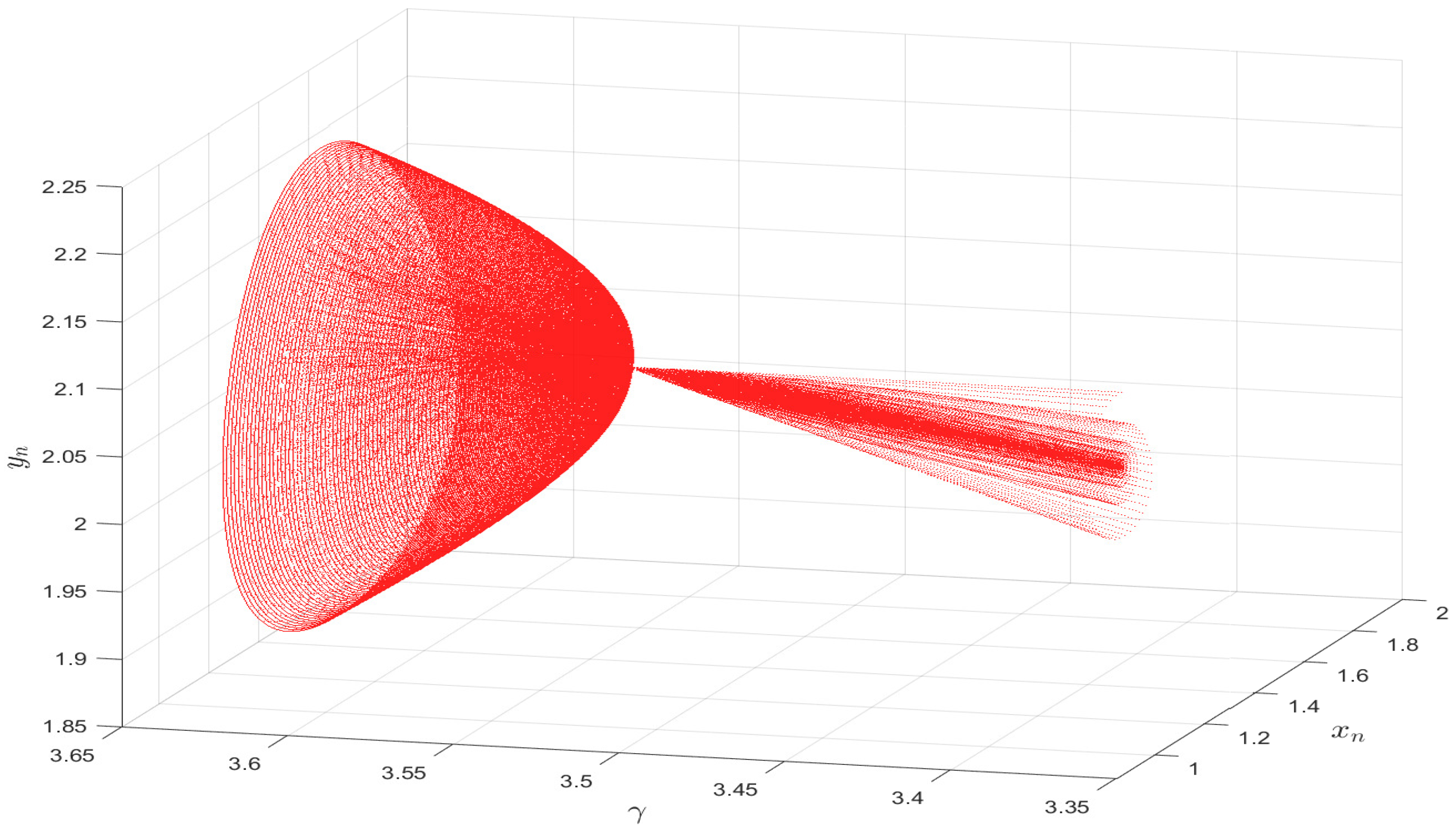
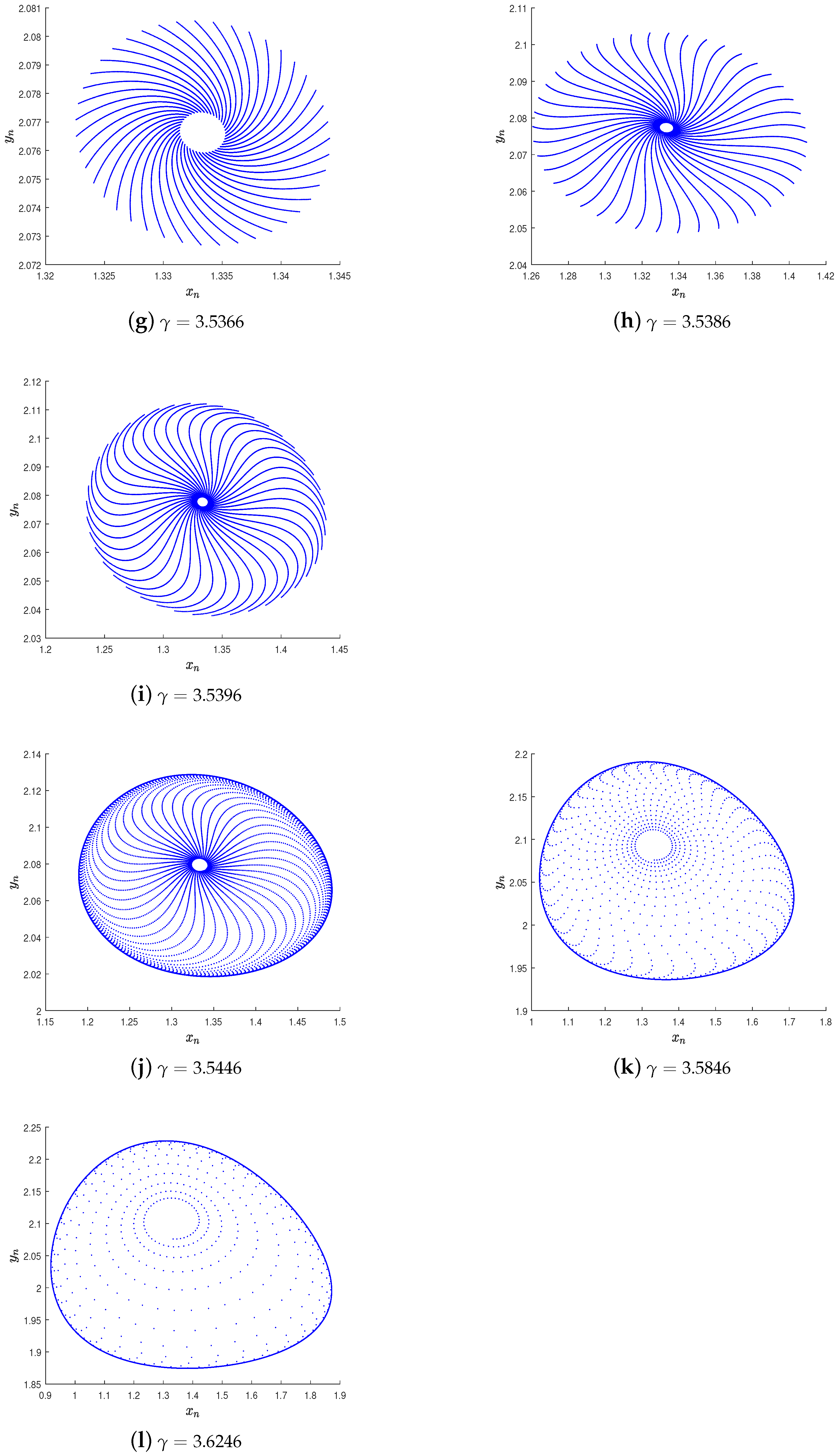
5. Numerical Simulation

In this section, numerical simulations are presented to verify the theories given above. Since our model is difference equations, and the iterative expressions are already given, there is no need to create novel calculations, such as interpolation methods in the case of differential equations. We assume that $\left(\beta ,c,\delta \right)=\left(0.2,0.3,0.08\right)$ and $\gamma \in \left(3.3,3.7\right)$, then system (3) undergoes Neimark–Sacker bifurcation around its positive equilibrium $\left(x_0,y_0\right)=\left(1.3333333,2.0759193\right)$ when $\gamma$ passes through the critical value ${\gamma }^{*}=3.2345912$. At $\left(\beta ,c,\delta ,\epsilon \right)=\left(0.2,0.3,0.08,3.2345912\right)$, the eigenvalues of system (3) are ${\lambda }_1=0.9893238+0.1457338i$ and ${\lambda }_2=0.9893238-0.1457338i$ with $\left|{\lambda }_1\right|=\left|{\lambda }_2\right|=1$.

From Figure 1, it can be seen that the model has a limit loop at $\left(x_0,y_0\right)$ as $\gamma$ changes, which means that the biomass of predators and prey will eventually form a cycle. From Figure 2, it is clear that, when $\gamma$ is chosen as the bifurcation parameter, $\left(x_0,y_0\right)$ of system (3) is locally focused when $\gamma <{\gamma }^{*}$. Furthermore, when $\gamma >{\gamma }^{*}$, there exist attracting closed invariant curves.

We assume that the parameters $\beta$ and $\delta$ are constant during the increasing of $\gamma$, which means that the growth rate of prey and the death rate of predators are unchangeable. Since $\gamma$ is proportional to the refuge parameter c (4), it is clear that, with the improvement of refuge ability, the quantitative relationship between predator and prey changes from constant to regular periodic.

6. Conclusions

Our work deals with the study of the local dynamical properties of a predator–prey system with discrete time (2) and Neimark–Sacker bifurcation associated with the periodic solution of system (3) improved by system (2). We proved that system (2) has three equilibria, and we provided their dynamical properties. Particularly, we focused on the stability and bifurcation situations of its unique positive equilibrium $\left(x^{*},y^{*}\right)=\left(\frac{\delta +\left(\alpha \delta -\beta \right)\xi }{\beta \left(1-c\right)-\delta },\left(\frac{1+\alpha \xi +x^{*}}{1-c}\right)\left(1-\frac{x^{*}}{\gamma }\right)\right)$ and presented a specific form of resolution and proof.

In addition, we proved that system (3) undergoes Neimark–Sacker bifurcation around its interior fixed point $\left(x_0,y_0\right)$ when the bifurcation curve is given as $S=\left\{\left(c,\beta ,\delta \right)\in {\mathbb{R}}_{+}^3:\gamma ={\gamma }^{*}=\frac{\delta +\beta \left(1-c\right)+\delta \left(\beta \left(1-c\right)-\delta \right)}{{\left(\beta \left(1-c\right)-\delta \right)}^2+\left(\beta \left(1-c\right)-\delta \right)},\left|D\right|<2\right\}$, where $D=\frac{x^{*}}{\gamma }\left(\frac{\gamma -x^{*}}{1+x^{*}}-1\right)+2.$ In order to verify the theoretical discussion, we also provided a numerical simulation at $\left(x_0,y_0\right)$ when the parameter is varied in a small neighborhood of $\gamma ={\gamma }^{*}$. When $\gamma >{\gamma }^{*}$, there exist attracting closed invariant curves from the positive equilibrium, which indicates that predators and prey can coexist under the periodic oscillations for an extended period of time.

In biology, with the improvement of refuge ability c, the quantitative relationship between predator and prey changes from constant to regular periodic, which means that slight growth of the refuge ability c destroys the original balance and better explains population attributes in nature. It appears that prey refuges not only ensure that prey do not become extinct but also promote interactions with predators and enhance population activity on a periodic scale. Therefore, we can precisely change the biological density of predators and prey to achieve the desired goal by regulating the number of refuge parameters c in relation to other variables according to one’s needs.

In subsequent work, other parameters can be considered for bifurcation studies to obtain conclusions of different biological significance. Alternatively, other discrete methods can be used to improve the model.

References

1. Lotka, A.J. Analytical Note on Certain Rhythmic Relations in Organic Systems. Proc. Natl. Acad. Sci. USA 1920, 6, 410–415. [Google Scholar] [CrossRef] [PubMed] [Green Version]
2. Volterra, V. Variazioni e Fluttuazioni del Numero d’Individui in Specie Animali Conviventi. Mem. R. Accad. Naz. Lincei. Ser. VI 1926, 2, 31–113. [Google Scholar]
3. Lotka, A.J. Contribution to the Mathematical Theory of Capture. Proc. Natl. Acad. Sci. USA 1932, 18, 172–178. [Google Scholar] [CrossRef] [Green Version]
4. Liu, C.; Zhang, Q.L.; Huang, J.; Tang, W.S. Dynamical Behavior of a Harvested Prey-Predator Model with Stage Structure and Discrete Time Delay. J. Biol. Syst. 2009, 17, 759–777. [Google Scholar] [CrossRef]
5. Samuelson, P.A. Generalized Predator-Prey Oscillations in Ecological and Economic Equilibrium. Proc. Natl. Acad. Sci. USA 1971, 68, 980–983. [Google Scholar] [CrossRef] [Green Version]
6. Liu, X.X.; Zhang, C.R. Stability and Optimal Control of Tree-Insect Model under Forest Fire Disturbance. Mathematics 2022, 10, 2563. [Google Scholar] [CrossRef]
7. Chen, H.Y.; Zhang, C.R. Dynamic analysis of a Leslie–Gower-type predator–prey system with the fear effect and ratio-dependent Holling III functional response. Nonlinear Anal. Model. Control. 2022, 27, 1–23. [Google Scholar] [CrossRef]
8. Liu, X.L.; Xiao, D.M. Complex dynamic behaviors of a discrete-time predator–prey system. Chaos Solitons Fractals 2007, 32, 80–94. [Google Scholar] [CrossRef]
9. Beretta, E.; Capasso, V.; Rinaldi, F. Global stability results for a generalized Lotka-Volterra system with distributed delays. J. Math. Biol. 1988, 26, 661–688. [Google Scholar] [CrossRef]
10. Hofbauer, J.; Thus, J.W. Multiple limit cycles for predator-prey models. Math. Biosci. 1990, 99, 71–75. [Google Scholar] [CrossRef] [PubMed] [Green Version]
11. Brauer, F.; Sánchez, D.A. Constant rate population harvesting: Equilibrium and stability. Theor. Popul. Biol. 1975, 8, 12–30. [Google Scholar] [CrossRef]
12. Cheng, L.F.; Cao, H.J. Bifurcation analysis of a discrete-time ratio-dependent predator–prey model with Allee Effect. Commun. Nonlinear Sci. Numer. Simul. 2016, 38, 288–302. [Google Scholar] [CrossRef]
13. Lai, L.Y.; Zhu, Z.L.; Chen, F.D. Stability and Bifurcation in a Predator-Prey Model with the Additive Allee Effect and the Fear Effect dagger. Mathematics 2020, 8, 1280. [Google Scholar] [CrossRef]
14. Sasmal, S.K. Population dynamics with multiple allee effects induced by fear factors—A mathematical study on prey-predator interactions. Appl. Math. Model. 2018, 64, 1–14. [Google Scholar] [CrossRef]
15. Kuznetsov, Y.A.; Rinaldi, S. Remarks on food chain dynamics. Math. Biosci. 1996, 134, 1–33. [Google Scholar] [CrossRef] [Green Version]
16. Aziz-Alaoui, M.A.; Okiye, M.D. Boundedness and global stability for a predator-prey model with modi-fied Leslie-Gower and Holling-type II schemes. Appl. Math. Lett. 2003, 16, 1069–1075. [Google Scholar] [CrossRef] [Green Version]
17. Chen, F.D.; Chen, L.J.; Xie, X.D. On a Leslie-Gower predator-prey model incorporating a prey refuge. Nonlinear Anal. Real World Appl. 2009, 10, 2905–2908. [Google Scholar] [CrossRef]
18. Hung, K.-C.; Wang, S.-H. A theorem on S-shaped bifurcation curve for a positone problem with convex–concave nonlinearity and its applications to the perturbed Gelfand problem. J. Differ. Equ. 2011, 251, 223–237. [Google Scholar] [CrossRef] [Green Version]
19. Hu, Z.Y.; Teng, Z.D.; Zhang, L. Stability and bifurcation analysis of a discrete predator–prey model with nonmonotonic functional response. Nonlinear Anal. Real World Appl. 2011, 12, 2356–2377. [Google Scholar] [CrossRef]
20. Zhang, C.R.; Zheng, B. Stability and bifurcation of a two-dimension discrete neural network model with multi-delays. Chaos Solitons Fractals 2007, 31, 1232–1242. [Google Scholar] [CrossRef]
21. Abdelaziz, M.A.M.; Ismail, A.I.; Abdullah, F.A.; Mohd, M.H. Bifurcations and chaos in a discrete SI epi-demic model with fractional order. Adv. Differ. Equ. 2018, 2018, 1–19. [Google Scholar] [CrossRef] [Green Version]
22. Ghosh, J.; Sahoo, B.; Poria, S. Prey-predator dynamics with prey refuge providing additional food to predator. Chaos Solitons Fractals 2017, 96, 110–119. [Google Scholar] [CrossRef]
23. Gladkov, S.O. On the Question of Self-Organization of Population Dynamics on Earth. Biophysics 2021, 66, 858–866. [Google Scholar] [CrossRef]
24. Li, W.; Li, X.Y. Neimark–Sacker Bifurcation of a Semi-Discrete Hematopoiesis Model. J. Appl. Anal. Comput. 2018, 8, 1679–1693. [Google Scholar] [CrossRef]
25. Li, X.Y.; Shao, X.M. Flip bifurcation and Neimark–Sacker bifurcation in a discrete predator-prey model with Michaelis-Menten functional response. Electron. Res. Arch. 2023, 31, 37–57. [Google Scholar] [CrossRef]
Figure 1. Invariant circles in response to the relationship between predator and prey biomass from the Neimark–Sacker bifurcation with x 0 , y 0 = 1.3333333 , 2.0759193 and bifurcation parameter γ varying from 3.3846 to 3.6246.
Mathematics 11 01399 g001
Figure 2. Phase diagrams of system (3) with parameters β , c , δ = 0.2 , 0.3 , 0.08 and x 0 , y 0 = 1.3333333 , 2.0759193 and with different values of γ .
Mathematics 11 01399 g002aMathematics 11 01399 g002b
Disclaimer/Publisher’s Note: The statements, opinions and data contained in all publications are solely those of the individual author(s) and contributor(s) and not of MDPI and/or the editor(s). MDPI and/or the editor(s) disclaim responsibility for any injury to people or property resulting from any ideas, methods, instructions or products referred to in the content.