Determining Dimensionality with Dichotomous Variables: A Monte Carlo Simulation Study and Applications to Missing Data in Longitudinal Research

Abstract

Dichotomous data correspond with various types of commonly encountered data, e.g., positive/negative, case/control, missing/observed, in many fields, including medicine, health, and social sciences. Despite their ubiquity, criteria for determining dimensionality from dichotomous variables are not yet established. We conducted a large-scale simulation (Study 1) to evaluate four criteria—Kaiser, empirical Kaiser, parallel analysis, and profile likelihood—to determine the dimensionality of dichotomous data across combinations of correlation matrices (Pearson r or tetrachoric ρ) and analysis methods (principal component analysis or exploratory factor analysis), and combinations of study characteristics: sample sizes (100, 250, and 1000), variable splits (10%/90%, 25%/75%, and 50%/50%), dimensions (1, 3, 5, and 10), and items per dimension (3, 5, and 10) with 1000 replications per condition. Parallel analysis performed best, recovering dimensionality in 87.9% of replications when using principal component analysis with Pearson correlations. Guidance for selecting criteria is provided. In Study 2, we applied this dimensionality reduction approach to two different longitudinal data sets where missing data posed difficulty for multivariate data analysis. The applications of this approach to longitudinal data suggest that the exploration of resulting missing data meta-patterns is useful in practice.

1. Introduction

Growing consensus establishes a set of criteria for determining the dimensionality of continuous variables under a variety of conditions [1,2], such as Kaiser’s criterion [3] and parallel analysis [4]. New methods, e.g., empirical Kaiser criterion [1], are also being presented in the literature that may outperform benchmark methods in some circumstances. Despite their ubiquity, criteria for determining dimensionality from dichotomous indicators are not yet established [5]. Although some previous research suggests the best approaches for determining the dimensionality of continuous indicators may not work as well with dichotomous indicators [2,6,7], these studies have typically considered only one analysis method (e.g., factor analysis), a selected few criteria, or a limited number of study conditions [8,9]. Furthermore, prior research has not subjected the same data sets to direct comparisons by different combinations of analysis methods and data matrices. It raises questions about whether these findings generalize across the range of conditions typical for research in the medical, behavioral, health, social, and educational sciences.

1.1. Dichotomous Data and Matrices

Dichotomous data arise across nearly every discipline and correspond with various types of commonly encountered data, e.g., positive/negative, case/control, and missing/observed. Such data are often conceptualized as resulting from an underlying continuous (e.g., Gaussian) distribution where the observation’s value is determined in relation to some underlying cut-point or threshold, equatable with a particular split in the data (e.g., 50%/50% or 10%/90%; or the difficulty parameter). The data matrix for each would be identical for comparable criteria, regardless of how the underlying data were conceptualized or generated.

Although dichotomous indicators are often treated as continuous in disciplines such as economics, conventional wisdom—backed with some previous research [10,11,12]—leads to an expectation that tetrachoric correlation coefficients outperform Pearson r for dichotomous data in some applications, such as data reduction [13,14]. Except under conditions reflecting relatively extreme splits in the data, we should generally expect differences to be relatively small since Gaussian, logit, and probit distributions largely overlap once standardized for differences in means and variances [15]. In the current study, we considered conditions for which these comparisons may not have been systematically evaluated by previous research. We evaluated all methods using both Pearson r and tetrachoric ρ coefficients.

1.2. Dimension Reduction

Researchers across disciplines frequently need to perform data reduction on dichotomous data matrices. We focus on two of the most widely used analyses that involve dimensionality determination, principal component analysis, and factor analysis (or principal axis factoring or exploratory factor analysis) because other approaches appropriate to dichotomous data, such as singular value decomposition [16] and non-negative matrix factorization [17], are not yet widely encountered in most areas of the medical, behavioral, educational, health, and social sciences. Likewise, we do not consider confirmatory approaches here, such as confirmatory factor analysis (CFA) [18], where dimensionality is specified a priori, or latent class analysis [19], which relies on very different approaches to determining dimensionality from the methods considered here [20] and can place considerable demands on sample sizes [21].

1.2.1. Principal Component Analysis

Principal component analysis (PCA) [22] seeks to reduce the dimensionality of multivariate data containing multiple inter-correlated variables in a way that retains maximal variation present in the data set. This is accomplished by a standardized linear projection which maximizes the variance in the projected space and also minimizes the squared reconstruction error [23]. As such, the first few principal components retain most of the variation present in the original set of variables. In other words, weights are applied to form linear combinations of the original variables, such that the first component has the largest inertia (i.e., variance), the second component is computed such that it is orthogonal to the first component and has the largest remaining variance, and so forth until the same number of components as the observed variables are computed [24]. A key decision for the researcher then is to determine the number of principal components to retain to accomplish the goal of sufficiently extracting the information with a parsimonious structure—a reduced set of principal components sufficient for the aims of the data reduction task (e.g., ≥X% variance recovered, identifying the most important signals in the data, denoising, etc.).

Important goals of the principal component analysis are to (1) extract the most important information from the multivariate data matrix, (2) reduce the data matrix by retaining only the orthogonal principal components with a maximal variance of the original data matrix, and thereby (3) clarify the structure of the observations and the variables in the multivariate data matrix (4) to denoise a dataset [24]. Therefore, for data reduction, PCA’s emphasis is on accounting for maximal variance rather than capturing maximal covariance or explaining inter-relations between observed variables in the original data matrix. Mathematically, the principal components are empirical aggregates of the inter-correlated observed variables, without much underlying theory about which variables should be associated with which components.

1.2.2. Factor Analysis

Factor analysis (FA), in contrast, hypothesizes a set of underlying latent common factors that potentially explain the associations among observed variables [25]. In a common factor model, the factors influence the observed variables (i.e., factor indicators), as modeled in the linear regression functions of observed variables, which are dependent on latent factors. The factors (i.e., predictors in the linear regressions) are shared among the observed variables with different regression coefficients (i.e., factor loadings), whereas the regression residuals, representing the variances unrelated to the common factors, are unique to the observed variables. As such, the total variance of an observed variable is partitioned into the variance contributed by the common factors (i.e., communality) and the variance unrelated to the common factor (i.e., uniqueness). Factor analysis estimates commonalities to minimize unique and error variance from the observed variables. This is a key difference from principal component analysis, which provides a mathematically determined empirical solution with all variances included. The key to estimating the varying factor loadings for different observed variables lies in the covariance (or correlation) structure among the original observed variables and the common-factor-model-implied covariance structure. Unlike principal component analysis, principal factor analysis is an analysis of the covariances among the observed variables in the original data matrix, and its purpose is primarily to seek the underlying theory (i.e., the common factors) about why the observed variables correlate to the extent they do.

Despite the distinctions in the goal of analysis and extraction technique, factor analysis is similar to the principal component analysis in its utility in reducing a large number of observed variables down to a few latent factors/components (i.e., the underlying dimensions). Factor analysis achieves a reduction in dimensions by invoking a common-factor model relating observed variables to a smaller number of common latent factors.

As noted above, PCA and FA differ in terms of their goals, objectives, purpose, and the kinds of applications to which they are best suited, but they are similar in terms of an essential step—determining dimensionality based on eigenvalue decompositions. For this reason, we compared the two analyses with the primary emphasis of correctly identifying the dimensionality of a set of dichotomous variables using different determination criteria.

1.3. Determining Dimensionality

There are vast literature on criteria for determining the dimensionality of multivariate variables that can be applied to data reduction approaches, e.g., principal component analysis and factor analysis. One of the most widely applied is the Kaiser criterion (also called the Kaiser-Guttman rule [3,26]), which retains all dimensions with eigenvalues greater than one (i.e., the dimensions that account for at least as much variance as a typical standardized item). The Kaiser criterion is the default approach in most statistical packages (e.g., SPSS), although some studies have suggested that this approach may lead to an over-extraction of components in many applications [27].

Kaiser’s method ignores the fact that eigenvalues are sorted from largest to smallest, thus capitalizing on chance differences associated with sampling variance. To address this issue, parallel analysis [4] uses data simulated under an independence assumption to subtract out this sampling error variance, and solutions can be evaluated using several different criteria (e.g., mean, median, and 95%^ile). Prior simulation studies have suggested that parallel analysis provides an unbiased estimate of the number of underlying dimensions and works well in practice, but its effectiveness is less clear with dichotomous indicators, such as in the current paper.

Quite recently, parallel analysis has been extended to consider data generated under data structures with varying numbers of dimensions in the Comparison Data method [16], with additional dimensions being added to the simulated data for as long as they produce a better agreement with the structure of the original data. We do not consider this method here because it (a) can be quite computationally intensive and (b) generally agrees quite well with results from parallel analysis; however, it represents a potentially important addition to the methods available for determining dimensionality.

In empirical contexts, many researchers rely on visual scree plots to determine the underlying dimensionality of multivariate data [28,29]. A plot of eigenvalues against the eigenvalue number is used to identify an “elbow” or “large gap” in the data at the point where the useful “signal” degenerates into noise or “scree”. However, this method provides no definite quantitative cutoffs and hence is difficult to use for empirical evaluation. The method of profile likelihood [30] attempts to address this shortcoming by quantifying the number of retained dimensions that maximize the observed data likelihood, thus providing an empirical method for determining the point at which a “gap” or “elbow” occurs within a scree plot.

Finally, an empirical Kaiser criterion (EKC) has recently been presented in the literature [1]. This approach is grounded in statistical theory and accounts for the serial nature of eigenvalues. In a Monte Carlo study [1], the EKC approach generally performed at least as well as parallel analysis, particularly with larger sample sizes and a smaller number of variables.

There has not been a consensus, however, on which criteria may perform well to determine the dimensionality of dichotomous variables in various circumstances. A recent simulation study indicated that, while parallel analysis generally performed well, it was not as effective in factor analysis with dichotomous indicators [8]. The root-mean-square error of approximation (RMSEA) adapted from the traditional use of confirmatory factor analysis was recommended to determine the number of factors [8]. However, the results also suggested that a lack of convergence may often be expected under the circumstances faced by applied researchers (e.g., smaller sample sizes and a larger number of variables), which would make it considerably less robust in applied research.

Similar to the approach using RMSEA, the Hull method also utilizes fit indices (e.g., comparative fit index) together with the degree of freedom, which is traditionally for confirmatory factor analysis, to assist in determining the number of underlying factors to extract for exploratory factor analysis [31]. Although a heuristic approach, the performance was largely dependent on the choice of a fit index to yield the Hull variant, which is suited for specific kind(s) of the model estimator. We do not consider the Hull method here due to the additional within-method conditions one needs to consider, which are not shared by dimension determination approaches, such as Kaiser, parallel analysis, and EKC.

To our knowledge, research effort on dichotomous data dimensionality criteria has focused on parallel analysis, but the findings were not conclusive. In an earlier simulation study [32], the researchers investigated parallel analysis as an approach to dimensionality determination for unidimensional dichotomous data. They found that with the 95th and 99th percentiles of random data eigenvalues as criteria, parallel analysis was accurate in identifying the unidimensionality in the simulated dichotomous variables. On the other hand, in a similar study [33] that evaluated parallel analysis in determining dichotomous variables sharing a single underlying dimension, the results did not agree. The researchers concluded that parallel analysis generally did not perform well with FA in determining unidimensionality among a set of dichotomous variables when a Pearson correlation matrix was analyzed, with the tetrachoric correlation matrix and parallel analysis providing somewhat better, but still unsatisfactory, results. Their findings also pointed to other influencing factors on the performance of parallel analysis, including sample size, and factor loadings.

1.4. Missing Data Indicators

One type of dichotomous variable in applied research is dichotomous missing data indicators, which are created by recoding all variables in an analysis to have two possible values, e.g., 1 = missing and 0 = not missing, to indicate whether a variable response is missing for a case. For instance, if there are 10 observed variables involved in the analysis, one would create 10 missing data indicators, each for one variable. Collectively, these 10 missing data indicators explicitly show all missing data patterns across the entire data set.

Missing data indicators and missing patterns are widely used in missing data approaches [34]. It is a top priority to describe and understand the missing data in a study prior to examining variables of primary research interest. Whereas there are well-established expectations regarding how to appropriately describe variables, few expectations or conventions exist for describing missing data using dichotomous missing data indicators. In addition, methods for handling missing data have become increasingly available to non-methodologists, and many software packages include routines for direct maximum likelihood or multiple imputation approaches that previously required considerable methodological sophistication to implement correctly. Systematic exploration of missing data mechanisms is critical to selecting and applying the most appropriate statistical techniques for the analysis of incomplete data [35,36].

1.4.1. Missing Data Indicators and Patterns

Following prior research on statistical analysis with missing data [37], we define the missingness indicator matrix, $M=\left(m_{ij}\right)$, where $m_{ij}=0$ if it is observed, and $m_{ij}=1$ if $Y_{ij}$ is missing. Each unique row of matrix $M$ defines a distinct missing data pattern. A study with $N$ observations and $k$ different variables can potentially result in up to ${min[N,2}^k]$ different missing data patterns, but observations missing on all $k$ variables clearly contribute no information about population parameters. On the other hand, the pattern “observed on all $k$ variables” is included in the overall consideration of missing data in a study and represents the subset of observations remaining after listwise deletion.

1.4.2. Missing Data Mechanisms

Missing data mechanisms represent our concerns about whether the probability that variables are observed is related to the underlying values of those variables. Rubin’s taxonomy [38] describes missing data as being Missing completely at random (MCAR), Missing at random (MAR), or Missing not at random (MNAR). Data are said to be MCAR if the probability of missingness does not depend on the values of covariates $\left(X\right)$, auxiliary $\left(V\right)$, or outcome $\left(Y\right)$ variables $\left(X,V,Y\right)$, i.e.,

$$Pr\left(M|X,V_{Obs},V_{Mis},Y_{Obs},Y_{Mis}\right)=Pr\left(M\right).$$

(1)

Data are typically only MCAR when missing data result from a priori design decisions, such as planned missing designs (e.g., XABC design [39]) and matrix sampling [40]. In contrast, data are MAR when missingness is independent of missing responses $Y_{Mis}$ and, conditioned on observed responses $Y_{Obs},V_{Obs}$ and covariates $X$, i.e., $Pr\left(M|X,V_{Obs},V_{Mis},Y_{Obs},Y_{Mis}\right)\hspace{0.25em}=\hspace{0.25em}Pr\left(M|X,V_{Obs},Y_{Obs}\right)$. Both MCAR and MAR data are said to be ignorable because when conditioned on the observables, the missing data mechanism does not need to be explicitly modeled in order to draw valid inferences. When missingness or nonresponse depends on the values of missing variables, conditioning on the observed variables, data are said to be MNAR, i.e., $Pr\left(M|Y_{Obs},Y_{Mis}\right)\hspace{0.25em}=\hspace{0.25em}Pr\left(M|Y_{Mis}\right)$. MNAR data are said to be nonignorable, and the missing data mechanism must be modeled explicitly. Research on missing data mechanisms additionally defines the condition of data being Observed at random (OAR) [41], which is a necessary but not sufficient condition for establishing that data are MCAR.

Missing data always introduce uncertainty about the unobserved values and their potential influence on study findings, much in the same way that sampling introduces uncertainty about population parameters, but one in which we typically do not have access to the sampling characteristics that would allow us to recover the population parameters fully. In this sense, if MCAR data comprise a simple random sample (meaning that no adjustments need to be made prior to analysis), then MAR would be analogous to sampling with stratification, oversampling, and/or clustering (meaning that both parameter estimates and standard errors may be biased without appropriate adjustments for sampling characteristics, which are known). Finally, MNAR data lie at an unknown point along the spectrum from the MAR case where sampling characteristics are at least partially known to convenience or snowball sampling (meaning that even after adjustments are made for known or suspected characteristics, results may still be biased in unknown ways). In the latter case, everything that can be learned about the missing data mechanism can aid in model specification.

1.4.3. Missing Data Indicators for Exploring Missing Mechanisms

It is important for researchers to understand how the results obtained appear to depend on the implicit or explicit assumptions being made about the unobserved values. Within the context of randomized controlled trials, which feature an experimental design, one or a very small number of discrete outcome variables, and a well-defined study end-point, reasonable advice and guidance are available [36,42,43,44,45,46]. These recommendations tend to focus on investigating a series of sensitivity analyses in order to better understand how assumptions about the missing data mechanism might affect study results [45]. In non-experimental contexts, there is a growing emphasis on sensitivity analyses in the analysis of missing data [42,46,47,48,49].

However, in longitudinal medical research, which is most often observational, longitudinal, and multivariate, very little systematic and concrete guidance currently exists for handling the large number of ways in which combinations of variables may jointly be observed or missing. Researchers looking for guidance in identifying patterns and predictors of nonresponse will typically find few concrete and systematic examples of how to proceed.

In order to evaluate several approaches to understanding missing data mechanisms, researchers analyzed data from five clinical trials using four different approaches [50]. They found considerable agreement across Little’s MCAR test [51], the test of random dropout [52], which are both mean-based, and the logistic regression methods [53,54]. Logistic regression is more useful in this context, however, because it also identifies potential auxiliary variables.

In a study of the association between dynamic experiences of poverty and children’s behavior problems across four waves of the National Longitudinal Study of Youth [55], researchers first identified discrete patterns of missing data using rotated principal component analysis and then examined variables associated with the probability of nonresponse in order to adjust models for selective nonresponse. A four-component solution accounted for 84 percent of the variance and yielded a clearly interpretable pattern of component loadings after oblique rotation. These missing data meta-patterns represented: Missing at Time 1, Missing at Time 2, Missing at Times 3 and/or 4 and/or demographic variables, and a very small group reflecting Missing on Mother’s Education and Past Poverty Experiences that was not pursued further). Next, a series of logistic regression models were estimated to predict missingness on the three patterns of missing data. Models used information contemporaneously collected and from previous waves to identify auxiliary variables for inclusion in subsequent analyses. Moreover, results considerably differed when analyzed by listwise deletion and with model-informed adjustments for selective non-response in ways that were clearly interpretable based on an understanding of the missing data mechanisms.

In another study, depressive symptom data from five waves of the Baltimore Longitudinal Study of Aging were analyzed [56]. There were no missing observations within waves, and when a participant dropped out of the study, he or she was not recontacted to participate in subsequent waves. Thus, all individuals missing at a particular wave were also missing on subsequent occasions, creating a monotone nonresponse pattern. This meant that no data reduction process was required in light of the limited number of ways in which individuals could have missing data. The authors used logistic regression analyses predicting non-response at each wave. Results indicated that older age and greater depressive symptoms were associated with a greater likelihood of dropout at all subsequent waves, but otherwise, there did not appear to be any systematic processes determining participant dropout. In particular, there were no gender differences in dropout rates in adjusted models. However, the authors were not able to explore differences as a function of reasons for dropout and attrition (e.g., mortality or ill health).

In a third study, albeit the different goals, researchers took a similar approach by using logistic regression models to evaluate evidence that data are OAR, as partial evidence in support of data being MCAR when no observed variables predict non-response [41]. From this perspective, the observed variables that were associated with the probability of non-response violate the OAR assumption without considering the potential to use variables significantly associated with non-response as the auxiliary variables in subsequent analysis.

1.4.4. An Eight-Step Approach to Describe and Understand Missing Data

Based on simulation study findings (Study 1 presented below) and the prior literature on missing data, we provide a set of practical guidelines for how to describe missing data patterns, examine missing data mechanisms, demonstrate their application, and recommend a few plausible follow-up steps towards making inferences about potential missing data mechanisms (

Table 1. A Systematic Approach to Reducing Missing Data Patterns and Inferring about Mechanism.

Purpose	Step	Operation
Data preparation	1	Create missingness indicator matrix: recode all variables in the data set into dichotomous missing data indicators (1 if missing or 0 if observed).
Data denoising and reduction	2	Perform PCA (or desired data reduction technique) on the missingness indicator matrix.
	3	Determine the dimensionality (i.e., meta-patterns) underlying the missing indicator matrix following guidelines by Study 1.
	4	Extract the dimension scores (e.g., principal component scores) and obtain the predicted scores.
	5	Examine distributions of component scores and classify observations using a sensible cutoff to indicate membership in a principal missing meta-pattern (Score ≤ threshold coded as 0, not missing, and score > threshold coded as 1, missing).
Examining missing data components to evaluate hypotheses about missing data mechanism	6	Examine distributions of both observed variables and the corresponding missing data indicators by meta-pattern and by the features of study design.
	7	Regress each meta-pattern on its missing indicators in a logistic regression model to examine plausible missing data mechanisms, e.g., ruling out OAR/MCAR.
	8	If no clear pattern emerges, repeat Steps 6–7 with some stratifying variable (e.g., treatment condition and gender) or in combination with other missing data meta-patterns

). The process consists of eight steps, from data preparation to missing data pattern denoising and reduction and finally to exploring plausible missing data mechanisms.

Step 1, the primary data preparation step, is to recode all analytic variables in a data set to the same number of missing data indicators to form the missingness index matrix. With the newly created missing data indicators, we can start with the missing data denoising and reduction following the next steps.

Step 2 is to perform PCA on missing data indicators obtained in Step 1.

Step 3 is to determine the number of principal components to retain using a method with the best performance (e.g., parallel analysis) based on the design characteristics (e.g., sample size, the number of items per dimension, and percentage of missing data) following the criteria selection guidelines in Study 1 (presented below).

Step 4 is to extract the desired number of principal components and obtain the predicted component scores from the statistical program that performs the PCA, including rotated solutions in cases where missing data components might be expected to correlate. These principal components represent the missing data meta-patterns that account for most of the total variations in the missing data indicators.

Step 5 is to categorize the component scores using a more sensible cutoff to indicate membership in each missing data meta-pattern, e.g., based on the component score distributions or based on a split at zero (score ≤ 0 coded as 0, not missing, and score > 0 coded as 1, missing). As opposed to the program-generated component scores, the dichotomous coding intuitively shows whether an individual response belongs in a missing data meta-pattern. By Step 5, the unwieldy number of missing data patterns has been reduced to a much smaller number of missing data meta-patterns.

Step 6 is to examine the distributions of observed variables and their corresponding missing data indicators by each component and each known characteristic of the study (e.g., refresher cohort, mortality, school dropout, and baseline scores) [55]. Recommended tests for this step include a t-test, chi-square, logistic regression, etc. The results of this preliminary screening show whether data differ by a main missing data pattern as indicated by the component score. Doing so by the known characteristics of study design also provides an evaluation of the external validity of the main missing patterns.

Step 7 is to predict dichotomized component scores from observed variables or their corresponding missing data indicators using binomial logistic regression or similar methods [56]. The results show the extent to which each main missing data pattern—as indicated by the component scores—depends on the observed variables where data are either missing or observed, suggesting the possibility of an NMAR mechanism.

If the pattern is still difficult to interpret in Step 8, stratify the sample by variables (e.g., gender and treatment condition) and then repeat Steps 6 and 7 for each subgroup, and even the data reduction step could potentially be independently conducted within each level of the group or stratification variable. We recommend this step in all situations with an experimental manipulation and/or stratification variable [57]. This is imperative for any models that will ultimately include the evaluation of one or more interaction terms. In some cases, it may be possible to learn more about reasons for missing data in a secondary data source by contacting its authors.

1.5. The Present Studies

We conducted a large-scale simulation study (Study 1) to determine which criteria were effective in reducing the dimensionality of multivariate dichotomous data under a variety of conditions, including sample size, percentage missing, number of dimensions, and the number of items per dimension. We then applied Study 1’s findings to reduce dimensions of dichotomous missing data indicators and further followed the eight-step approach to understand missing data in two longitudinal studies. We conclude by discussing the feasibility, theoretical, practical contributions, and limitations of our approach and conclude with a few suggestions for making inferences about plausible missing data mechanisms based on the reduced missing data patterns as well as potentially fruitful directions for future research.

2. Study 1

The purpose of Study 1 was to evaluate the performance of different methods for correctly determining the dimensionality underlying a set of dichotomous indicators across a range of conditions typical for multivariate medical, social, behavioral, and educational research. Specifically, we conducted a large-scale simulation to evaluate four criteria (Kaiser’s criterion, empirical Kaiser’s criterion, parallel analysis, and profile likelihood) for determining the dimensionality of dichotomous variables given combinations of methods (principal component analysis or exploratory factor analysis) and matrices (Pearson r or tetrachoric ρ), sample sizes (100, 250, and 1000), variable splits (10%/90%, 25%/75%, and 50%/50%), underlying dimensions (1, 3, 5, and 10), and items per dimension (3, 5, and 10) with 1000 replications per condition. We focused on determining dimensionality because it is established in an identical fashion for both PCA and FA.

2.1. Materials and Methods

2.1.1. Design

To consider a range of conditions typical of many real-world applications with dichotomous variables (e.g., 0/1, incorrect/correct, and observed/missing), we used a factorial design. Between-subjects factors, which represent various characteristics of study data, included: (1) the number of underlying dimensions—1, 3, 5, or 10; (2) the number of items per dimension—3, 5, or 10; (3) sample size—100, 250, or 1000; and (4) dichotomous variable splits—90%/10%, 75%/25%, or 50%/50%. Within-subjects factors, which represent researcher-selected analytic approaches, were: (i) correlation matrix—Pearson r or tetrachoric ρ, and (ii) analysis method—PCA or FA.

2.1.2. Outcomes

We evaluated four different criteria for determining dimensionality—the number of underlying dimensions. These included: (1) empirical Kaiser criterion (EKC), (2) Kaiser criterion, (3) parallel analysis with 95%ile criterion, and (4) the profile likelihood. We considered a criterion successfully performed in a specific condition if it recovered the correct number of underlying dimensions in at least 95% of replications.

2.1.3. Data and Procedure

Between-Subject. We constructed 1000 replications in each condition with distinct between-subject factors, for example, 1000 replications with (1) one underlying dimension, (2) three items per dimension, (3) N = 250, and (4) a 10%/90% split. Population correlations were set at 0.70 within variables on the same dimension, 0.30 between variables on different dimensions, and all data were drawn from multivariate normal distributions. Consistent with our hypothesized latent variable model, data were dichotomized via a probit link function. Variables were dichotomized based on whether observed values of the function exceeded the threshold associated with the population %ile cut-point for that condition.

Within-Subject. For each replication, the dichotomous data matrix was converted to correlation matrices (Pearson r and tetrachoric ρ) and analyzed by principal component analysis (PCA) and principal axis factoring (PAF or FA). The number of dimensions indicated by each criterion was determined for each of the four combinations of the correlation matrix and analysis method.

Whether the dimensionality was correctly recovered was determined for each criterion under each combination of method and matrix. A nominal indicator (1 = parallel analysis, 2 = empirical Kaiser, 3 = Kaiser, and 4 = profile likelihood) was constructed with the value referring to the criterion that performed best in a condition.

2.1.4. Statistical Analysis

Descriptive statistics and factorial analysis of variance (ANOVA) were used to examine the association of each between- and within-subject factor with the recovery of the correct number of dimensions. Factorial ANOVA was in preference to logistic regression owing to the large number of conditions where some criteria performed perfectly, which can lead to estimation difficulties with likelihood-based techniques. We also conducted a recursive partitioning analysis (or classification and regression trees [CART]) [58] to classify the simulation results, with tree pruning based on the minimum value of Mallow’s Cp. The R statistical package [59] was used for all data simulations and analyses. All code and data generated are available on an online data repository (blinded URL).

2.2. Results

2.2.1. Convergence

Convergence is achieved for 99.98% of data sets, regardless of the matrix-analysis combination. Failed convergence occurs only for N = 100 and when the split is 10%/90%. The lowest convergence rate (98.6%) is when N = 100, with one underlying dimension, three items per dimension, and a 10%/90% split, likely due to variables having insufficient variance/covariance for analysis.

2.2.2. Criterion Performances

Parallel analysis is the best-performing criterion of the four (all > 86%;

Table 2. Percentage of Replications with Dimensionality Correctly Determined by the Four Criteria Given Method and Correlation Matrix.

Analysis	Correlation	Criteria-Averaged	EKC	Kaiser	ParaAn	ProfLik
PCA	Pearson	77.0%	79.3%	73.4%	87.9%	67.4%
PCA	Tetrachoric	71.1%	73.7%	73.7%	86.2%	50.8%
FA	Pearson	67.5%	58.9%	63.9%	86.1%	61.1%
FA	Tetrachoric	61.4%	77.3%	76.7%	44.1%	47.4%

Note: Boldfaced indicates the method/criterion that performed the best with each combination. PCA = principal component analysis and FA = factor analysis.

) in all combinations of matrix and analysis, except in PAF/ρ, where EKC is the criterion that correctly determined dimensionality for the most replications (77.3%). Note, however, the performance of dimension determination criteria not only varies across the four matrix-analysis combinations as shown above but also differs by the between-subject factors. This calls for a detailed examination of performances by sample size, the number of underlying dimensions, the number of items per dimension, and the variable split, within a combination of matrix and analysis type, which we elaborate on below.

Among the four matrix-analysis combinations, PCA/r has the highest average percentage of correctly-recovered replications (77.0%; Table 1), and in this combination, the best-performing criterion—parallel analysis—correctly determines the highest percentage of replications (87.9%) compared with any criterion in any other matrix-analysis combination. Given these results, we present the detailed evaluation of criteria only for the combination of PCA with Pearson r. The full results are available as Table S1 of the Supplementary Material for researchers whose application suggests a different combination.

2.2.3. Criterion Performances Given PCA with Pearson r

Our design includes four between-subject factors: three sample sizes × four numbers of underlying dimensions × three numbers of items per dimension × three splits of variable values, which created a total of 108 conditions given the combination of PCA and Pearson r (and 432 conditions overall). Due to a large number of replications, ANOVAs indicate that all model effects are statistically significant using α = 0.05, including the five-way interaction. For this reason, we summarize the key findings and influences for each criterion.

Parallel Analysis. Parallel analysis performs the best among the four criteria given the PCA/r combination. Parallel analysis’s performance is driven primarily by sample size and the number of underlying dimensions. The parallel analysis correctly recovers the number of underlying dimensions at least 95% of the time under all 36 conditions when N = 1000, 31 of 36 conditions when N = 250, and 14 of 36 conditions when N = 100. PA also performs less well when the number of underlying dimensions is larger (e.g., 10 dimensions). The next influential factor is the number of items per dimension. Most of the failing cases for parallel analysis occur when given fewer items per dimension. The dichotomous value split does not matter for the performances of PA.

Empirical Kaiser Criterion. The performance of the empirical Kaiser criterion is primarily driven by sample size and a dichotomous value split. Better performances are observed when sample sizes are larger (e.g., 1000) and with a more even split (e.g., 50%/50%). The next influential factors are the number of underlying dimensions and items per dimension. EKC performs better when there are fewer underlying dimensions and fewer items per dimension.

Overall, EKC does not outperform parallel analysis as a criterion for determining the dimensionality of dichotomous variables in most conditions examined in the present study. The only conditions where EKC correctly determines the number of underlying dimensions in more replications than parallel analysis is when N = 100 or 250, the true number of dimensions is 3, 5, or 10, and when given three items per dimension.

Kaiser. The performance of the Kaiser criterion is primarily driven by sample size and the number of items per dimension. Better performances are observed given a larger sample size and few items per dimension. The next influential factors are the number of underlying dimensions (favoring fewer), followed by the dichotomous value split (favoring a more even split).

Overall, the Kaiser criterion does not outperform parallel analysis as a criterion for determining the dimensionality of dichotomous variables in most conditions we examined. It only outperforms parallel analysis in the same conditions where EKC also outperforms parallel analysis, in which its performances are not as well as EKC.

Profile Likelihood. The performance of profile likelihood is primarily driven by the number of underlying dimensions. With a greater number of underlying dimensions, profile likelihood performs better. The next influential factor is the sample size, favoring a larger sample size. Overall, profile likelihood does not outperform parallel analysis as a criterion for determining the dimensionality of dichotomous variables in almost all conditions we examined in the present study.

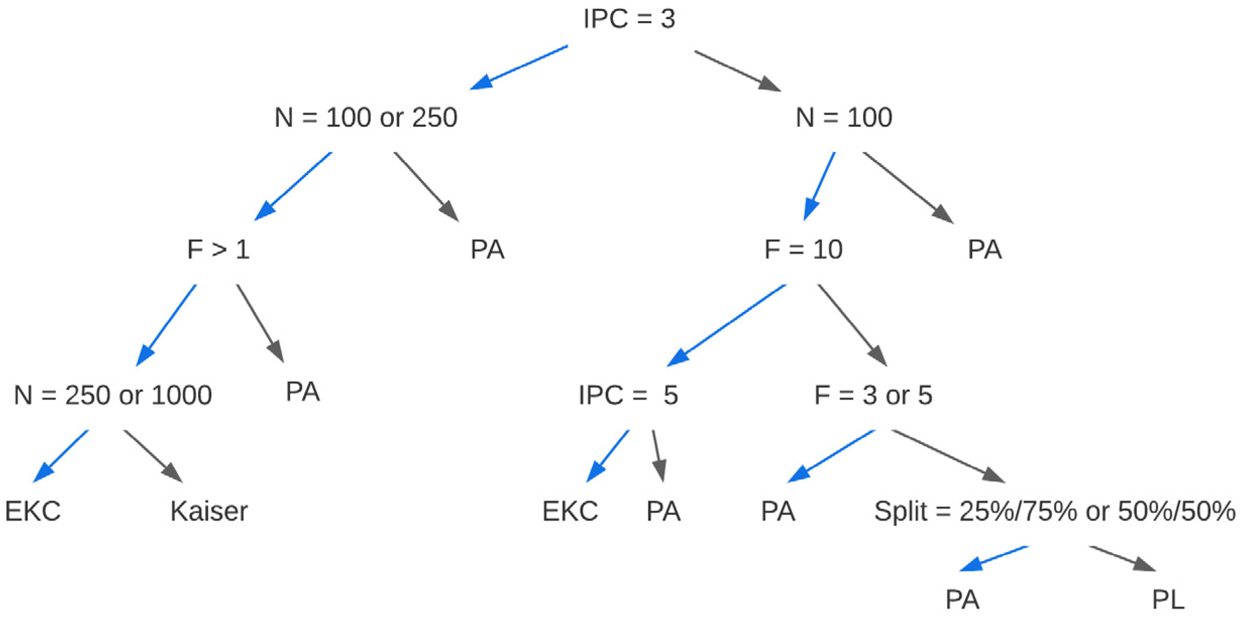
2.2.4. Guidance for Selecting a Criterion

We obtained a classification and regression tree from the PCA with r results (Figure 1). Our data support using parallel analysis given PCA with Pearson correlations, except in four scenarios. First, use EKC when there are 3 items per dimension, >1 underlying dimension, and N = 250. Second, use the Kaiser criterion when there are 3 items per dimension, >1 underlying dimension, and N = 100. Third, use EKC when there are 5 or 10 underlying dimensions, N = 100, and 5 items per dimension. Finally, use profile likelihood only when the underlying structure is unidimensional with 10 items per dimension, N = 100, and the value split is an extreme 10%/90%. We note that, in this case, the profile likelihood (99.5%) outperforms parallel analysis (93.1%) only by a small degree (see Figures S1–S3 for the CART for the other three matrix-analysis combinations).

Although parallel analysis generally outperforms the other methods under most circumstances when PCA is used with Pearson r, researchers should consider the closest scenario to their own from the conditions considered in our simulation. Then, dimensionality should be determined using one or all of the acceptable criteria for that combination of conditions, and in situations where there is disagreement, a sensitivity analysis should be performed to make a final determination.

2.3. Discussion

Accurate dimensionality determination is critical across a range of disciplines and applications and represents the first and most critical step in data reduction, but guidance is not well established for dichotomous data. Without clear criteria for first determining the dimensions underlying the large set of dichotomous variables, subsequent steps (e.g., factor/component rotations) cannot be carried out, and further analytic goals (e.g., data reduction and obtaining factor scores) cannot be achieved. This large-scale simulation study examined the performance of four criteria (i.e., parallel analysis, EKC, Kaiser, and profile likelihood) for determining the dimensionality of dichotomous variables under a considerably wider range of conditions than previous research. Specifically, we used a factorial design with four between-subject factors—sample size, number of underlying dimensions, number of items per dimension, and variable value split. More importantly, this is the first study, to our knowledge, that directly compares criterion performance across combinations of methods of analysis (principal component analysis vs. factor analysis) and the type of matrix analyzed (Pearson correlations vs. tetrachoric correlations).

Our findings suggest that the dimensionality of a dichotomous-variable data matrix is best determined using the combination of PCA with a correlation matrix based on Pearson r, regardless of how the data will be ultimately analyzed. This is important because numerous disciplines (e.g., educational testing, clinical assessment, and personality research) [2,6,32,33,60] heavily rely on dichotomously scored measures and computationally-intense tetrachoric ρ, which has risks of over-estimating linear relations. We also find that parallel analysis is the criterion that most frequently recovers the correct underlying dimensionality, expanding on prior research [1,32] on parallel analysis of continuous variables to that of dichotomous or dichotomous variables as a reliable approach to dimensionality determination. We highlight important findings below.

FA was originally developed to identify common factors among normally distributed continuous variables [61]; however, many assessments and questionnaires are made up of dichotomous or ordered categorical items [5]. The prior literature calls EFA with categorical variables “item factor analysis (IFA)” [2]. Conceptually, the least-squares approach to IFA is based on the assumption that underlying each categorical indicator is a normally distributed continuous latent response variable [5,62]. An individual’s standing on this latent variable relative to a set of thresholds determines which response category they fall into. For example, for a dichotomous item, if the individual’s standing on the latent response variable is below a certain threshold, they will endorse a score of zero, whereas if they are above this threshold, they will endorse a score of one.

Previous comparisons of criteria for dimensionality determination with dichotomous data have concluded that FA with tetrachoric correlations outperforms FA with Pearson correlations [13,14]. Our results corroborated performance under these conditions but further demonstrated that the results for dimensionality determination are also the poorest under precisely these conditions. Instead, the parallel analysis combined with PCA using Pearson correlations most often correctly determines dimensionality. We note that this does not in any way detract from the application of FA with dichotomous data, which likely should be performed using tetrachoric correlations once dimensionality is established to recover factor structure correctly.

In several regards, the results of Study 1 differ from conventional wisdom, perhaps due to the broader range of conditions we considered and perhaps also because we compared criterion performance across methods and matrices head-to-head on identical data sets. Most importantly, these results suggest that it is not necessary or beneficial to use tetrachoric correlation matrices in preference to Pearson r for the purposes of dimensionality determination, regardless of the combination of method and matrix ultimately used for analysis. Again, we believe that this should generally be the case except in situations with extreme splits on dichotomous variables or other potentially ill-conditioned circumstances [15,63]. This is important because numerous fields and disciplines heavily rely on dichotomously scored measures. For example, ability testing in educational settings and symptom assessment in clinical psychology are often based on questionnaires in which responses can fall into either one of two categories (i.e., correct/incorrect and symptom present/symptom absent), and the computationally intense tetrachoric have often been used for analyses of these dichotomous data, which may cause issues such as difficulty in estimation and over-estimation of linear relationships [64].

Another finding that can be considered surprising is that, for the purposes of dimensionality determination, PCA outperforms FA. This is important because, in educational and psychological research, factor analysis is primarily used in developing validity arguments for scales and theory development (e.g., intelligence, personality, and executive functioning) [27] because of its focus on identifying the underlying latent constructs that lead to correlations among the observed variables. Dimension reduction is both a necessary step toward the research goal and an inevitable byproduct of the process. On the other hand, principal component analysis is used to achieve a parsimonious summary of high-dimensional, multivariate data, so, arguably, data reduction is the most important goal of PCA. These results suggest that, although common practice is to exclusively apply either PCA or FA to a dataset for the entire analysis, it might be more effective, particularly in exploratory contexts, to use PCA for dimensionality determination, regardless of whether PCA or FA will ultimately be used to answer substantive research questions.

A third important finding from the current study is that parallel analysis is the criterion that most frequently recovers the correct dimensionality. Traditional FA and the tools used to guide determinations of dimensionality were developed for use with continuous data, and the application of these techniques to categorical data, especially dichotomous data, can lead to more suspect and difficult-to-interpret results [6,7,65]. For example, a parallel analysis might be less effective when scales contain dichotomous items [2,9]. Parallel analysis can also be effective but is less accessible for models with categorical indicators [66] and has also demonstrated a tendency to over-factor in certain circumstances or under-extract in others [9,67]. However, contrary to these concerns, our large-scale simulation results generally indicated a more accurate performance of parallel analysis for dichotomous variable dimensionality determination in various conditions tested.

In specific circumstances, EKC and Kaiser (and, in a unique condition, profile likelihood) may be the most effective criteria to use. Some researchers consider using the Kaiser criterion to determine dimensions a common mistake with factor analysis [27]. This is somewhat surprising since the prior literature has shown that the Kaiser criterion tends to extract too many dimensions in FA with continuous variables [68]. However, as a method to determine the dimensionality of multivariate dichotomous data, the traditional Kaiser criterion and its recent extension showed good performance in some conditions.

3. Study 2

In Study 1, the principal components reflect statistically principled and systematically derived ways in which one of the two dichotomous values tends to co-occur among multivariate variables. In the case of dichotomous missing data indicators, the principal components represent distinct underlying missing data meta-patterns. Empirically, we would expect that when data are MCAR, the missing data meta-pattern indicator would not be associated with any observed characteristic (or external information, as available). When data are MAR, the missing data component indicator would be associated with one or more observed characteristics (but not external information, as available). When data are MNAR, the missing data component indicator may be associated with one or more observed characteristics and external information as available. In the latter two cases, any variables that significantly predict a missing data component score will need to be included in subsequent statistical models related to variables loading on that component. Combinations of missing data components can also be used to create distinct missing data groups for analysis via, e.g., a pattern-mixture model.

We applied and evaluated the dichotomous data reduction process in Study 1 using two real-world longitudinal health-related data sets, where the underlying missing data mechanism(s) are either unknown or only partially known: (Application 1) longitudinal psychiatric clinical trial data analyzed by Hedeker and Gibbons [57], and (Application 2) self-report data on depressive symptoms in the Health and Retirement Study (HRS) [69]. The first study was selected because it was extensively studied as an example of MNAR data (subsequently analyzed via pattern-mixture models). The second study was selected because it added different cohorts of participants in different waves and had complex skip patterns within each wave, guiding whether self-report data would be collected from specific individuals in specific waves. Thus, we could analyze missing data patterns from the self-report component and independently validate our results by aligning the components with our expectations based on the study design that was external to the data analyzed.

3.1. Application 1

3.1.1. Data Source

The first application of our systematic eight-step approach used data from a well-known psychiatric clinical trial. The original study [57] analyzed data on changes in the severity of illness in the National Institute of Mental Health Schizophrenia Collaborative Study to illustrate the influence of missing data with a pattern-mixture approach. The target variable was Item 79, Severity of Illness, on the Inpatient Multidimensional Psychiatric Scale (IMPS79). Responses were on a scale of 1 (normal, not at all ill) to 7 (among the most extremely ill), which were treated in the analysis as continuous variables. Participants (N = 437) were grouped by placebo vs. drug; the main measurements occurred at Weeks 0, 1, 3, and 6.

To fully describe the missingness of this application example, we report on the missingness by variable, sample size, and by missing patterns. We analyzed the missingness on IMPS79_0, IMPS79_1, IMPS79_3, and IMPS79_6 (“H&G data set” hereafter), which have 0.7–23.3% missing data across occasions. Of the total 437 cases, 73.5% have complete data, and 26.5% have missing data on at least one occasion. Given the four variables, the maximum number of missing patterns is 15 (i.e., 2⁴ − 1, excluding the pattern missing on all variables). In reality, the H&G data set showed nine missing data patterns (see missing patterns in Table S2 of Supplementary Materials).

This data set has the advantage of having a sample size and a percentage of missing data that are quite typical for longitudinal medical and psychology research. This study design is also typical for the kinds of randomized controlled trials studied in health sciences and psychology. Additionally, the original study provided conclusions about the missing data mechanism and, hence, an excellent reference for evaluating our missing data reduction approach.

Hedeker and Gibbons’ own approach reduced the missing patterns to one—missing at Week 6 or not—which was found to be non-ignorable due to the significant interaction between dropout and assignment to drug treatment condition on the changes in IMPS79 scores over time (b = −0.635, SE = 0.196, and p = 0.002; p. 71). Specifically, for the completers (i.e., observed through Week 6) across all four measurements, both patients on the drug and on placebo experienced decreases in IMPS79 scores, and the decrease was greater for the completers on the drug than for those on placebo. For the dropouts (i.e., missing at Week 6), the patients on the drug experienced a significant decrease in IMPS79 scores, whereas those on placebo did not experience much decrease.

3.1.2. Procedure

We sought to reduce the missing data patterns of the H&G data set and then evaluate hypotheses about missing data mechanisms following our eight-step approach (Table 1). First, we recoded IMPS79_0, IMPS79_1, IMPS79_3, and IMPS79_6 into corresponding dichotomous missing data indicators, IMPS79.0m, IMPS79.1m, IMPS79.3m, and IMPS79.6m (Missing = 1 or Observed = 0), respectively; performed principal component analysis on the missing data indicators; used the four methods to determine the number of principal components to extract; and decided the most appropriate number of dimensions to extract from these data (Steps 1–3). Next, we extracted the component, calculated the predicted component scores, and dichotomized the component scores to make dichotomous indicators of data missing or not on the principal components (Steps 4–5). Finally, we analyzed the changes in IMPS79 scores by drug, by the principal missing meta-pattern (or “Component 1”), and the interaction between drug and component, and compared our findings to the original study [57].

3.1.3. Results and Discussion

Based on Study 1, all four determination criteria (i.e., EKC, Kaiser, parallel analysis, and profile likelihood) correctly determine the number of dimensions for more than 99% of the simulated data that share similar characteristics to the H&G data set, i.e., N = 250, 1 principal component, 3 or 5 variables per component. Among the four methods (

Table 3. Number of Dimensions Determined by the 4 Criteria for Application Data Sets.

Application Data Set	EKC	Kaiser	Parallel Analysis	Profile Likelihood
Hedeker and Gibbons (1997)	1	1	1	1
CES-D Data of the HRS	4	4	4	2

Note: Boldface indicates the criteria correctly determines the number of dimensions for 100% of simulated data in Study 1 with similar characteristics to the application data set.

), parallel analysis and profile likelihood correctly determine the number of dimensions for 100% of the simulated data. Thus, we expected one principal component to be extracted with the H&G data set (i.e., N = 437, 4 variables, and 1.5–54.6% of missing observations).

We conducted PCA on the four missing data indicators and found that the four criteria unanimously indicated one component to be extracted. This finding supports our expectations based on Study 1. The indicator, missing at Week 0, does not significantly load on the principal component (=−0.130, p > 0.05), the indicator, missing at Week 1, significantly but moderately loaded on the component (=−0.300, p < 0.05), but missing at Week 3 and missing at Week 6 significantly and strongly loaded on the component (=0.863 and 0.838, respectively, p < 0.001). These two high loadings suggest that the predominant missingness in the data set is mainly due to missing data in Weeks 3 and 6. This result is to a large extent consistent with the pattern—missing at Week 6—as found in the original study, but suggests that differences between completers and attritors may actually be discernible by Week 3.

We estimated component scores and, based on inspection of their distribution (which was essentially bimodal), dichotomized them into Component 1 (0 coded as 0, Not Missing, and >0 coded as 1, Missing). To examine how well our extracted component described the missingness, we compared our Component 1 to a known reference—the pattern found in the original study. Specifically, we modeled the changes in IMPS79 scores from Week 0 to Week 6 using mixed models with three covariates: (a) Drug (on drug vs. on placebo), (b) Component 1 (Missing vs. Observed at Weeks 3–6), and (c) the Drug–Component 1 interaction. Results indicate that both the main effect of the Drug and the Drug–Component 1 interaction is significant on changes in IMPS79 scores (b = −0.521, SE = 0.127, p < 0.001; and b = −0.514, SE = 0.225, p = 0.022, respectively), whereas the main effect of Component 1 on changes in IMPS79 scores is nonsignificant (b = −0.113, SE = 0.188, and p = 0.547).

These findings are largely consistent with the original study. Our Component 1, which represents missing data in Weeks 3–6, is associated with changes in IMPS79 scores (i.e., a component–treatment interaction). As shown in the prototypical trajectories (Figure 2), for the completers, participants on placebo and on drug start very similarly at Week 0, but those on the drug have a significantly greater decrease in IMPS79 scores. For the dropouts (missing since Week 3), despite similar starting points, their difference in decreases is predicted to be much larger than that with the completer pair, favoring the dropouts among individuals assigned to the drug treatment.

Our findings highlight the crucial role of missingness at Weeks 3–6 (i.e., principal missing indicator, Component 1) in the estimated decrease of illness severity, as the missingness interacts with the treatment condition, creating differential effects of the drug for those who completed all waves vs. those who were missing since Week 3. Our principal missing meta-pattern—although obtained by a very different and purely-empirical approach from the original—helps infer that the data are highly likely MNAR and sheds light on the differential effects of assignment to the intervention group, which is quite consistent with the original study.

3.2. Application 2

3.2.1. Data Source

A second application used the interview data on depressive symptoms from 10 waves (1992 through 2010) of the Health and Retirement Study (HRS) [69]. The HRS is a large, nationally representative multi-wave survey containing detailed information on a wide range of topics. Baseline data for the HRS were first collected in 1992 through face-to-face interviews conducted with respondents aged 51–61 (birth cohort 1931–1941) and their spouses. The original sample consisted of 7600 households and more than 12,600 persons and was based on a multistage area probability design oversampling Hispanics, African Americans, and Florida residents. The response rate was over 80%. Follow-ups are biannually performed by telephone, with proxy exit interviews for deceased individuals. Additional cohorts were added to the sample beginning in 1998, drawn from the Aging and Health Dynamics in the Oldest Old (AHEAD [70], born 1923 or before), Children of the Depression Age (CODA, 1924–1930), and War Babies (WB, 1942–1947). The total sample size in the HRS for the waves considered was 31,169. Thus, individuals would have missing data for waves before their cohort was recruited. Similarly, individuals would not be given self-report questionnaires on these items under various circumstances (e.g., deceased or cognitively impaired).

Our analytic variables selected from the extensive study database were those on depressive symptoms, as measured by the Center for Epidemiological Studies Depression (CES-D) scale. The HRS uses a subset of eight items from the original 20-item version of the Center for Epidemiological Studies Depression (CES-D) scale. In terms of the structure of the CES-D items assessed in the HRS, there is representation from the three most important of the four CES-D subscales. Specifically, there are three items (depressed, lonely, and sad) from the depressed affect (DA) subscale, two items (happy and enjoyed life) from the positive affect (PA) subscale, and three items (effort, sleep, and get going) from the somatic complaint (SO) subscale (interpersonal symptoms are not represented). The resulting variables examined in the present study were subscale scores on depressed affect (DA), positive affect (PA), and somatic complaint (SO) for each wave, which makes a total of 30 variables over 10 waves (“CES-D data set” hereafter).

Of the 31,169 cases in the HRS study, 3868 (12.4%) cases have missing data on all 30 variables (but valid data on other variables not considered here), which results in an analytic sample size of 27,301 for the CES-D data set. Of the analytic sample, 18.2% have complete data across all 10 waves, and 81.8% have missing data for at least one variable. Given the 30 variables, the maximum number of missing patterns is 1,073,741,823 (i.e., 230-1). We observed 898 missing data patterns, which is far from the maximum but still an unwieldy number of missing data patterns (see Table S2 of Supplementary Materials).

The CES-D data set provides the opportunity to evaluate our approach with data on many variables derived from multiple waves with a large sample of 27,301 participants. Another advantage of using these data from the HRS is that the study design features and participant status account for some missingness in known ways and are available to data users. For example: (1) cohorts were added to the study in various waves; (2) vital status is known for this sample of older adults; and (3) physical or cognitive impairment precluded completion of various self-report measures for some individuals in some waves. This information is housed in a separate study-wide tracking database—the HRS Tracker file (Tracker 2016, Early Version 3.0)—which contains demographic information, interview status, and if, when, and how an interview was conducted in each wave. Therefore, after we adopted our approach to extract influential missing data meta-patterns without assistive information outside of the 30 variables, we were able to compare the meta-patterns in the CES-D data set (i.e., whether data were, in fact, observed) to the participant status records in the Tracker file (i.e., whether participants were supposed to provide data), and thereby validate our approach.

3.2.2. Procedure

We sought to reduce 898 observed missing data patterns and evaluate our hypotheses about the missing data mechanisms using our eight-step approach (Table 1). First, we recoded the 30 CES-D variables into 30 corresponding missing data indicators, from DA1m to SO10m (Missing = 1 or Observed = 0), performed a principal component analysis on the missing data indicators, used the four methods to determine the number of principal components to extract, and decide the most appropriate number of dimensions to extract from these data (Steps 1–3). Next, we extracted the components, calculated the predicted component scores, and dichotomized the principal component scores to make a dichotomous variable indicating whether variables were missing or observed (Steps 4–5).

To use the missing data meta-patterns to make inferences about potential missing data mechanisms, we utilized the HRS Cross-Wave Tracker data set (Tracker 2016, Early Version 3.0). We conducted logistic regressions of each dichotomous component on 10 index variables (i.e., from index01 to index10) that indicate whether a participant was supposed to provide data on these variables at each wave. We created these 10 variables based on variables provided in the Tracker data set, including the participant’s vital status (i.e., alive), whether a proxy provided interview data for the participant (i.e., proxy, which indicates that self-reported CES-D data should not be collected), whether interview data was obtained in a given wave (i.e., iwwave), and the year when first interviewed (i.e., firstiw). Each index variable shows whether a participant’s CES-D data should be missing or observed at a measurement occasion for the HRS study design reasons (Should be Missing = 1, Should be Observed = 0). For instance, the variable index03 represents whether or not a participant’s CES-D data should be missing in 1996 (wave 3 of the HRS): If a participant was interviewed before or in 1996 for the first time and was alive in 1996, her interview data were self-reported within this wave, and her interview data were not provided by a proxy, then this participant’s CES-D data should not be missing in 1996, and her index03 = 0 (i.e., Should be Observed). If any of the above-mentioned conditions were not met, then her index03 = 1 (i.e., Should be Missing; see

Table 4. Participant Status in HRS as Shown by Tracker 2016.

Variable	Year	Expected Status	N	Percentage %
index01	1992	Observed	12,004	38.5
		Missing	19,165	61.5
index02	1994	Observed	10,691	34.3
		Missing	20,478	65.7
index03	1996	Observed	10,225	32.8
		Missing	20,944	67.2
index04	1998	Observed	19,341	62.1
		Missing	11,828	37.9
index05	2000	Observed	17,517	56.2
		Missing	13,652	43.8
index06	2002	Observed	16,130	51.8
		Missing	15,039	48.2
index07	2004	Observed	18,327	58.8
		Missing	12,842	41.2
index08	2006	Observed	17,209	55.2
		Missing	13,960	44.8
index09	2008	Observed	16,077	51.6
		Missing	15,092	48.4
index10	2010	Observed	14,164	45.4
		Missing	17,005	54.6

Note: Index01–Index10 were created using variables in the Tracker 2016 (Early Version 3.0) of the HRS (N = 31,169), which were independent of the CES-D data set. Variables include vital status, whether interviewed within wave proxy status, and the year of the first interview. Should be observed = 0 and Should be missing = 1.

for distributions).

3.2.3. Results and Discussion

Based on Study 1, three dimensionality determination criteria—EKC, Kaiser, and parallel analysis—correctly determine the number of dimensions for 100% of the simulated data similar to the CES-D data set, i.e., N = 1000, three or five principal components, 5 or 10 variables per component, and 50% missing data (Table 3). In Study 1, the largest sample size we simulated was N = 1000, so we compared the CES-D data set with these simulated data. The performance with data sets of N = 1000 is extremely close to 100% correct; therefore, we expected the performance with the CES-D data set to be similar, given similarities in other aspects, i.e., the number of principal components, the number of items per dimension, and percentage of missing data. Thus, we expected three, four, or five components to be extracted with the CES-D data set (i.e., N = 27,301, a total of 30 variables, and 38.1–67.2% missing observations) based on the more accurate EKC, Kaiser, or parallel analysis methods.

We conducted a principal component analysis on the 30 dichotomous missing data indicators and found that three criteria unanimously indicate four components (Table 3). These findings confirmed our expectations based on Study 1. We then estimated rotated component scores and dichotomized them to create Components 1 to 4 (score $\le$ 0 coded as 0, Not Missing; and score > 0 coded as 1, Missing), reducing 898 missing data patterns to 4 main patterns for the CES-D data set, each of which is structured around missing data across contiguous waves of data collection.

We also considered the three- and five-component solutions with sensitivity analyses. The three-component solution separated waves 1 through 3, waves 4 through 6, and waves 7 through 10, whereas the five-component solution separated waves 1 through 3, waves 4 and 5, waves 5 and 6, waves 7 through 9, and waves 9 and 10. Each of these can be identically analyzed to what follows.

To validate how well the four extracted missing data meta-patterns describe missingness, we conducted four logistic regression models of Components 1 through 4, each on the 10 index variables created using variables of the HRS participation status in the separate Tracker data file, which was not used to in the previous steps to generate the four components. All four models successfully converge and provide a better fit to the data than the corresponding null models with only the intercept (

Table 5. Logistic Regressions of Each Component on the 10 Index Variables Tracker 2016 of HRS.

	Component 1	Component 2	Component 3	Component 4
LR ${\chi }^2$(df)	42,068.21 (10)	42,134.44 (10)	41,316.56 (10)	40,214.77 (10)
AUC	0.999	1	0.999	1
Sensitivity	99.7	99.8	99.5	99.8
Specificity	99.5	99.9	99.9	99.4
% Correct	99.6	99.8	99.7	99.6
Intercept	−11.71 c	−16.01 c	−7.19 c	−16.74 c
Index01	−1.69 c	−1.74 c	0.29	5.26 c
Index02	0.26	−0.4	−0.39	11.96 c
Index03	0.97 b	2.23 c	−1.11 b	11.43 c
Index04	0.87 b	18.80 c	−3.90 c	−0.59
Index05	−1.01 c	13.07 c	−0.13	0.25
Index06	−5.99 c	12.73 c	6.07 c	−0.58
Index07	−4.19 c	−3.66 c	16.10 c	0
Index08	7.02 c	−1.530 c	8.35 c	0.65
Index09	8.11 c	−0.15	1.22 c	−0.06
Index10	16.40 c	0.73 a	−5.67 c	−0.47

Note: ^a p < 0.05, ^b p < 0.01, and ^c p < 0.001. Boldface indicates the three strongest predictors for each component.

). The models all have high sensitivity, specificity, and an overall rate of correct classification close to one. Because the variables used to construct the y-side and x-side variables in these models are independently constructed, it provides considerable evidence for the validity and potential utility of this approach for understanding missing data mechanisms in practice.

The odds ratios in the logistic regressions suggest results consistent with findings from PCA: Component 1 is linked with those who should be missing at waves 9–10, Component 2 is associated with those who should be missing at waves 4–6, Component 3 is associated with those who should be missing at waves 7–8, and Component 4 is linked with those who should be missing at waves 1–3, with a small shared association between C1 and C3 at wave 8, and a shared association between C2 and C3 at wave 6. For example, a participant had index01 = 1, index02 = 1, and index03 = 1, which means she should not be providing data at waves 1–3 based on the design of the HRS. Our approach showed that she had Component 4 = 1 and all other components = 0, correctly identifying that her CES-D scores at waves 1–3 were missing. That is, according to study design information from the HRS Tracker file, this participant was not enrolled in the HRS until wave 4. Our approach to obtaining the four missing patterns (i.e., the four components), although it was purely empirical and did not utilize any study design information, accurately captures the four main missing patterns that reflect the missingness induced through the recruitment design of the HRS over this period.

4. General Discussion

This study makes three primary contributions to longitudinal and multivariate research in medicine and social sciences. Study 1’s findings provide a large-scale empirical head-to-head evaluation of four criteria for determining the dimensionality of multivariate dichotomous data under a range of conditions typical in medical, social, behavioral, and psychological research. Second, based on the simulation results and the prior literature on missing data, we present an eight-step approach to systematically reduce a potentially large number of missing patterns (formed by dichotomous missing indicators) to a much smaller, manageable number of missing data meta-patterns, to assist further understanding of missing data. Third, in Study 2, we applied the eight-step approach to validation using two published data examples and successfully obtained empirical support for the eight-step approach, effectively and efficiently providing a clear and concise presentation of missingness and assisting in further handling of missing data, which would remove obstacles for analyzing data of research interests.

Increasing accessibility of methods for the analysis of missing data has not yet been matched by strong consensus on methods for systematically evaluating the assumptions on which successful application of these methods rests. In medical, psychological, social, and educational research, data are often multivariate and longitudinal, which requires a reasoned approach to data reduction prior to the examination of missing data mechanisms because the number of potential missing data patterns exponentially grows with the number of variables in the analysis.

In terms of the problem of systematically reducing missing data patterns to a more manageable number of meta-patterns, we evaluated the systematic eight-step approach using real data examples representing a wide spectrum of conditions. Under nearly all conditions, our results point to some clear and concrete recommendations. Consistent with the broader literature on component extraction [8,71], our results suggest that parallel analysis should be the preferred method under most circumstances considered here. This method recovers the correct number of dimensions in over 95% of cases under every condition we studied using simulated data for sample sizes of at least 250. This intermediate sample size is “typical” across many disciplines, suggesting that the approach we outline here is likely to be effective in most circumstances encountered by researchers. For applications that appreciably differ from the range of conditions considered in the present study, applying our approach to a small, tailored simulation is straightforward.

Although the method we describe is agnostic regarding the underlying missing data mechanisms, we also found evidence that this approach yielded a small number of missing data meta-patterns that could, in turn, be used to explore potential missing data mechanisms, including providing novel insights when data are known or suspected to be MNAR, as our application illustrated.

Our systematic missing data approach is also likely to be useful for public-use data sets that are increasingly distributed with multiple imputations for missing values. Several examples exist of a multiple imputation approach with large-scale data sets. An approach like the one we outline here could be very useful when coupled with popular approaches, such as multiple imputations using chained equations. Whereas some authors have favored a “kitchen sink” approach to imputation [36], we would expect that a more limited and principled approach would ultimately be favored in the bias–variance tradeoff. In addition to identifying auxiliary variables that can be used in subsequent analyses, combinations of missing data meta-patterns can also be used to identify groups for use in pattern-mixture models.

Missing data always introduce uncertainty about unobserved values. In the best circumstances, they do so in a similar fashion to the way that analysis of data from a sample introduces uncertainty about parameters in the population, but informative non-response can have considerable consequences for study conclusions if not more fully evaluated. Further, methods for the analysis of MNAR data are still emerging, and this problem has been theoretically shown to be intractable based only on the observed data. For this reason, recommendations for analyses with missing data increasingly revolve around sensitivity analyses. This shifts the emphasis toward methods that reduce, or at least better characterize, the extent of a potential bias for key predictors of interest. Of particular interest is the extent to which study conclusions depend on the assumptions, implicit or explicit, being made about the nature of unobserved values.

The systematic but exploratory missing data analysis approach we recommend here is strongly consistent with a sensitivity analysis framework in two ways. First, the examination of associations with a smaller number of missing data “meta-patterns” (i.e., the lower dimensionality) allows each to be considered in greater depth, alone and in combination. We have outlined a minimal set of specific and systematic recommendations that can be used to guide this process for a given number of missing data components that are also easy to extend and tailor to different contexts. Second, we also advocate consideration of different numbers of missing data meta-patterns (e.g., k ± 1). In many cases, results agree very closely across these conditions. In circumstances where results diverge, this is important information that can be used to guide sensitivity analyses and to qualify results appropriately.

4.1. Limitations

Although we considered a much wider range of conditions than most previous research addressing this topic, we only considered a single set of correlations among and within dimensions. Future research should consider more complex data structures. These include different correlation structures, combinations of oblique and orthogonal dimensions (components or factors), deviations from simple structure, and even ordered categorical latent variables and finite-mixture models.

Our approach is also compatible with researchers conducting similar simulations that more closely align with their own data. In real data applications, we do not know the ground truth, so we cannot truly evaluate performance with real data. However, our results with real data are both broadly interpretable and consistent with the previous analyses that are available for two of the data sets we considered here, and the simulation model we used here can easily be applied to any specific combinations of factors of interest.

Another important consideration is that study results, particularly adjustments for factors associated with the missing data mechanism, are only going to be as good as the quality of ancillary data available. This might suggest that researchers should devote greater attention to collecting additional follow-up data from participants as possible, something that has long been recommended practice in the field of survey research.

4.2. Future Directions

This study presents one validated approach to promote more systematic consideration of missing data mechanisms in multivariate and/or longitudinal contexts, but considerable opportunities remain for better aligning missing data theory and practice, particularly for highly multivariate. For example, our missing data mechanisms had a known structure for the simulated data but not for the real data applications. Future research should examine the performance of these procedures using real data with deliberately masked observations under a variety of conditions.

Similarly, in many areas of research, such as the analysis of clinical trial data, there is legitimate concern about missing data methods that can be “gamed” or manipulated by the data analyst. This can sometimes lead to the widespread adoption of some less favorable but more objective treatments of missing data, such as the last-observation-carried-forward method. Although this is one of our goals in presenting this approach in as systematic and replicable a manner as possible and situating it explicitly within an exploratory data analysis and sensitivity analysis framework, future research should carefully evaluate where missing data protocols need to be modified to further remove or reduce subjectivity in the application of missing data methods.

5. Conclusions

Study 1 provided empirical evidence for criteria to use for dimensionality determination—the first and most important step in a variety of data reduction techniques. We directly compared the performance of four widely used criteria in a variety of study conditions and given the different combinations of analysis methods and types of matrix analyzed. Our result supported using PCA with a Pearson correlation matrix as the preferred approach in determining how many dimensions that underlie a large set of dichotomous variables for a variety of circumstances examined.

Applying results from Study 1 to real data examples in a specific case of dichotomous variables—missing data indicators—we also presented a novel systematic and flexible procedure that can be used to facilitate exploration and evaluation of missing data meta-patterns in contexts with multivariate and/or longitudinal data commonly encountered in longitudinal medical research contexts. Using Study 1 to guide the dimensionality determination of dichotomous missing data indicators, we investigated potential missing data mechanisms and performed sensitivity analyses when considering the assumptions about missing data for study conclusions. As demonstrated in Study 2, the eight-step approach presented can easily be adapted to specific study or design characteristics to provide results more tailored than the conditions considered here.