Article

A Modified q-BFGS Algorithm for Unconstrained Optimization

1
International Business School, Shaanxi Normal University, Xi’an 710119, China
2
Department of Mathematics, Institute of Science, Banaras Hindu University, Varanasi 221005, India
3
Centre for Digital Transformation, Indian Institute of Management, Ahmedabad 380015, India
*
Author to whom correspondence should be addressed.
Mathematics 2023, 11(6), 1420; https://doi.org/10.3390/math11061420
Submission received: 27 January 2023 / Revised: 10 March 2023 / Accepted: 12 March 2023 / Published: 15 March 2023
(This article belongs to the Special Issue Optimization Algorithms: Theory and Applications)

Abstract

:
This paper presents a modification of the q-BFGS method for nonlinear unconstrained optimization problems. For this modification, we use a simple symmetric positive definite matrix and propose a new q-quasi-Newton equation, which is close to the ordinary q-quasi-Newton equation in the limiting case. This method uses only first order q-derivatives to build an approximate q-Hessian over a number of iterations. The q-Armijo-Wolfe line search condition is used to calculate step length, which guarantees that the objective function value is decreasing. This modified q-BFGS method preserves the global convergence properties of the q-BFGS method, without the convexity assumption on the objective function. Numerical results on some test problems are presented, which show that an improvement has been achieved. Moreover, we depict the numerical results through the performance profiles.

1. Introduction

There are many methods for solving nonlinear unconstrained minimization problems [1,2,3,4,5], most of them are variants of the Newton and quasi-Newton methods. Newton’s method uses the specification of the Hessian matrix, which is sometimes difficult to calculate, whereas the quasi-Newton method uses an approximation of Hessian. Over time, several attempts have been made to improve the effectiveness of quasi-Newton methods. The BFGS (Broyden–Fletcher–Goldfarb–Shanno) method is a quasi-Newton method for solving nonlinear unconstrained optimization problems, which is developed by Fletcher [6], Goldfarb [7], Shanno [8], and Broyden [9]. Since the 1970s, the BFGS method has become popular and is considered an effective quasi-Newton method. Some researchers have established that the BFGS method achieves global convergence under the assumption of convexity on the objective function. Mascarene has been shown with an example that the standard BFGS method fails with exact line search for non-convex functions [10]. Using inexact line search, some authors [11,12] established that the BFGS method achieves global convergence without the assumption of convexity on the objective function.
Quantum calculus (q-calculus) is a branch of mathematics and does not require limits to derive q-derivatives; therefore, it is also known as calculus without limits. In quantum calculus, we can obtain the q-derivative of a non-differentiable function by replacing the classical derivative with the q-difference operator, and if we take the limit q 1 , then the q-derivative reduces to the classical derivative [13]. Since the 20th century, quantum calculus has been linking physics [14] and mathematics [15] that span from statistical mechanics [16] and quantum theory [17] to hyper-geometric functions and number theory [14]. Quantum analysis was first introduced in the 1740s when Euler wrote in Latin about the theory of partitions, also known as additive analytic number theory.
At the beginning of the 19th century, Jackson generalized the concepts of classical derivatives in the context of q-calculus, known as Jackson’s derivative, or q-derivative operator, or q-difference operator or simply q-derivative [18]. He systematically developed quantum calculus based on pioneer work by Eular and Henie. His work introduced functions, mean value theorems [19], Taylor’s formula and its remainder [20,21], fractional integrals [22], integral inequalities and generalizations of series in the context of q-calculus [23]. The first time Soterroni [24] introduced the q-gradient vector. To obtain this, instead of the classical first order partial derivative, the first order partial q-derivative obtained from the q-difference operator is used.
In unconstrained optimization first time, Soterroni [24] used the q-derivative to establish the q-variant of the steepest descent method. After that, he also introduced the q-gradient method for global optimization [25]. In recent years, some authors have given some numerical techniques in the context of q-calculus to solve nonlinear unconstrained optimization problems [26,27,28]. In these methods, instead of a general gradient, a q-gradient is used because it permits the descent direction to work in the broader set of directions to converse rapidly.
Moreover, optimization has a crucial role in the field of chemical science. In this field, optimization methods have been used to minimize the energy consumption process in plants, design optimum fluid flow systems, optimize product concentration and reaction time in systems, and optimize the separation process in plants [29,30,31]. Some authors [32,33] have shown that the BFGS method is systematically superior in obtaining stable molecular geometries by reducing the gradient norm in a monotonic fashion. In a similar way, the modified q-BFGS algorithm can be used to find stable molecular geometries for large molecules.
In this paper, we modify the q-BFGS method for nonlinear unconstrained optimization problems. For this modification, we propose a new q-quasi-Newton equation with the help of a positive definite matrix, and in the limiting case, our new q-quasi-Newton equation is close to the ordinary q-quasi-Newton equation. Instead of calculating the q-Hessian matrices, we approximate them using only the first order q-derivative of the function. We use an independent parameter q ( 0 , 1 ) and quantum calculus based q-Armijo–Wolfe line search [34] to ensure that the objective function value is decreasing. The use of q-gradient in this line search is responsible for escaping the point from the local minimum to the global minimum at each iteration. The proposed method is globally convergent without the convexity assumption on the objective function. Then, numerical results on some test problems are presented to compare the new method with the existing approach. Moreover, we depict the numerical results through the performance profiles.
The organization of this paper is as follows: In Section 2, we recall essential preliminaries related to the q-calculus and the BFGS method. In the next section, we present a modified q-quasi-Newton equation, and using this, we give a modified q-BFGS algorithm and discuss its properties. In Section 4, we present the global convergence of the modified q-BFGS method. In the next section, we present numerical results. Finally, we give a conclusion in the last section.

2. Preliminaries

In this section, we reviewed some important definitions and other prerequisites from q-calculus and nonlinear unconstrained optimization.
Let q ( 0 , 1 ) , then, a q-complex number is denoted by [ b ] q and defined as follows [14]:
[ b ] q = q b 1 q 1 , b C .
A q-natural number [ m ] q is defined as follows [13]:
[ m ] q = 1 + q + + q m 1 , m N .
In q-calculus, the q-factorial [14] of a number [ m ] q is denoted by [ m ] q ! and defined as follows:
[ m ] q ! = [ 1 ] q [ 2 ] q [ m 1 ] q [ m ] q , m N
and
[ 0 ] q ! = 1 .
The q-derivative ( q 1 ) [18] of a real-valued continuous function f : R R , provided that f is differentiable at 0, is denoted by D q f and defined as follows:
D q f ( x ) = f ( x ) f ( q x ) ( 1 q ) x , if x 0 f ( x ) , if x = 0 .
If provided that f is differentiable on R then in the limiting case (q→1), the q-derivative is equal to classical derivative.
Let f : R n R be a real continuous function, then for x = ( x 1 , x 2 , , x n ) R n , consider an operator ε q , i on h as
( ε q , i f ) ( x ) = f ( x 1 , x 2 , , q x i , x i + 1 , , x n ) .
The partial q-derivative [22] of f at x with respect to x i , denoted by D q , x i f and defined as follows:
D q , x i f ( x ) = f ( x ) ( ε q , i f ) ( x ) ( 1 q ) x i , if x i 0 f ( x ) x i , if x i = 0 .
In the same way, higher order partial q-derivatives are defined as follows:
D q 0 = f ( x ) , D q , x 1 k 1 , , x i k i , x n k n m f ( x ) = D q , x i D q , x 1 k 1 x i k i 1 , , x n k n m 1 f ( x ) , where k 1 + k 2 + + k n = m and m = 1 , 2 , ,
Then, the q-gradient [24] of f is
( q f ( x ) ) = D q , x 1 f ( x ) , , D q , x i f ( x ) , , D q , x n f ( x ) T .
To simplify the presentation, we use A > 0 ( 0 ) to denote any n × n symmetric and positive definite (semi-definite) matrix A, use f : R n R to denote a real-valued function, use g q ( x ) to denote the q-gradient of f at x, use | | x | | to denote Euclidean norm of a vector x R n , use A k to denotes the q-quasi-Newton update Hessian at x k , throughout this paper.
Let f : R n R be continuously q-derivative then consider the following unconstrained optimization problem:
min x R n f ( x ) .
The q-BFGS method [34] generates a sequence { x k } by the following iterative scheme:
x k + 1 = x k + α k d q k ; k { 0 } N ,
where α k and d q k are step length and q-BFGS descent direction, respectively.
The q-BFGS descent direction is obtained by solving the following linear equation:
g q k + A k d q k = 0 ,
where A k is the q-quasi-Newton update Hessian. The sequence A k satisfies the following equation:
A k + 1 δ k = γ k ,
where δ k = x k + 1 x k and γ k = g q k + 1 g q k . In the context of q-calculus, we refer to the Broyden–Fletcher–Goldfarb–Shanno (BFGS) update formula as the q-BFGS update formula. Thus, the Hessian A k is updated by the following q-BFGS formula:
A k + 1 = A k A k δ k ( δ k ) T A k ( δ k ) T A k δ k + γ k ( γ k ) T ( δ k ) T γ k ,

3. Modified q-BFGS Algorithm

We modify the q-BFGS algorithm using the following function [35]:
f k ( x ) = f ( x ) + 1 2 ( x x k ) T B k ( x x k ) ,
where B k is a positive definite symmetric matrix. We obtain the following new q-quasi-Newton equation by using the function f k to the q-quasi-Newton method in the kth iterate:
A k + 1 δ k = λ k ,
where λ k = γ k + B k δ k . If we take k and δ k 0 , our new q-quasi-Newton equation is similar to the ordinary q-quasi-Newton equation. Using the above modification of the q-BFGS formula, we obtain the new one as follows:
A k + 1 = A k A k δ k ( δ k ) T A k ( δ k ) T A k δ k + λ k ( λ k ) T ( δ k ) T λ k ,
where λ k = γ k + B k δ k .
To provide a better formula, the primary task of this research is to determine how to select a suitable B k . We direct our attention to finding B k as a simple structure that carries some second order information of objective function. In this part, we will discuss a new choice of f and assume it to be sufficiently smooth.
Using the following quadratic model for the objective function [36,37], we have
f ( x ) f ( x k + 1 ) + ( g q k + 1 ) T ( x x k + 1 ) + 1 2 ( x x k + 1 ) T G k + 1 ( x x k + 1 ) ,
where G k + 1 denotes a Hessian matrix at point x k + 1 .
Hence,
f ( x k ) f ( x k + 1 ) ( g q k + 1 ) T δ k + 1 2 ( δ k ) T G k + 1 δ k .
Therefore,
( δ k ) T G k + 1 δ k 2 ( f k f k + 1 + ( g q k + 1 ) T δ k ) , = 2 ( f k f k + 1 ) + ( g q k + 1 + g q k ) T δ k + ( δ k ) T γ k ,
where f k denotes the value of f at x k .
By using (5), we have
( δ k ) T A k + 1 δ k = ( δ k ) T λ k = ( δ k ) T γ k + ( δ k ) T B k δ k .
The combination of Equations (9) and (10) shows that the reasonable choice of B k should satisfied the following new q-quasi-Newton equation:
( δ k ) T B k δ k = μ k ( μ k = 2 ( f k f k + 1 ) + ( g q k + 1 + g q k ) T δ k ) .
Theorem 1.
Assume that B k satisfies (11) and A k is generated by (6), then for any k,
f ( x k ) = f ( x k + 1 ) + ( g q k + 1 ) T ( x k x k + 1 ) + 1 2 ( x k x k + 1 ) T A k + 1 ( x k x k + 1 ) .
Proof. 
The conclusion follows immediately using Equations (10) and (11). □
The function f holds the Equation (12) without any convexity assumption on it and any formula derived from the original quasi-Newton equation fails to satisfy the Equation (12). From Equation (11), a choice of B k can be defined as follows :
B k δ k = η k , η k = μ k ( δ k ) T v k v k .
In above Equation (13), v k is some vector such that ( δ k ) T v k 0 .
By the Equations (2) and (3), we know that if δ k = 0 then g q k = 0 . Therefore, for all k we can always assume that δ k 0 ; otherwise, at the k t h iteration, the algorithm terminates. Hence, we can choose v k = δ k . Taking v k = δ k in the Equation (10), we have a choice of B k as follows:
B k = μ k δ k 2 I ,
where the norm is the Euclidean norm and μ k = 2 ( f k f k + 1 ) + ( g q k + 1 + g q k ) T δ k .
Remark 1.
The structure of B k is very simple, so we can construct and analyze it easily. We only need to consider the value of B k δ k to calculate the modified A k + 1 from the modified quasi-Newton Equation (5). Thus, once v k is fixed, different choices of B k , which satisfied (13) gives the same A k + 1 .
For computing the step length following q-gradient based modified Armijo–Wolfe line search conditions [34] are used:
f ( x k + α k d q k ) f ( x k ) + σ 1 α k ( d q k ) T g q k ,
and
q f ( x k + α k d q k ) T d q k σ 2 ( d q k ) T g q k ,
where 0 < σ 1 < σ 2 < 1 . Additionally, if  α k = 1 satisfies (16), we take α k = 1. In the above line search, a sufficient reduction in the objective function and nonacceptance of short step length is ensured by (15) and (16), respectively.
A good property of Formula (6) is that A k + 1 inherits the positive definiteness of A k as long as ( δ k ) T λ k > 0 ; provided that f is convex and step length is computed by an above line search. However,  when f is a non-convex function, then the above line search does not ensure the condition ( δ k ) T λ k > 0 . Hence, in this case, A k + 1 is not necessarily positive definite even if A k is positive definite. Therefore, some extra caution updates should be introduced as follows:
Define the index set K as follows:
K = k : ( δ k ) T λ k δ k 2 ϵ g q k c ,
where β [ ϑ 1 , ϑ 2 ] , with  0 < ϑ 1 ϑ 2 and ϵ are positive constants. We determine A k + 1 by the following rule:
A k + 1 = A k A k δ k ( δ k ) T A k ( δ k ) T A k δ k + λ k ( λ k ) T ( δ k ) T λ k if k K A k if k K .
Corollary 1.
Let B k be chosen such Equation (13) holds and A k is generated by (18), then A k + 1 > 0 , k N { 0 } .
Proof. 
Without loss of generality, let g k 0 , k . We use mathematical induction on k to prove this corollary. Since B 0 is chosen as a positive definite symmetric matrix, the result holds for k = 0 . Let’s assume that the result holds for k = n. We consider the case when k = n + 1 . If k K , then from Equations (17) and (18), ( δ k ) T λ k > 0 holds. Hence, for k = n + 1 , the result also holds. If k K , then by our assumption, A k + 1 = A k is also positive definite. This completes the proof. □
From the above modifications, we introduce the following Algorithm 1:
Algorithm 1 Modified q-BFGS algorithm
Require: 
Objective function f : R n R , ϵ is tolerance for convergence. Select an initial point x 0 R n , fix q ( 0 , 1 ) , and an initial positive definite symmetric matrix A o R n × m .
Ensure: 
With the corresponding objective value f ( x * ) , the minimizer x * is encountered.
1:
Set A 0 = I n .
2:
for k = 0,1,2... do
3:
    if  g q k < ϵ  then
4:
        Stop.
5:
    else
6:
        Solve the Equation (3) to find a q-descent direction d q k .
7:
        Find a step length α k satisfying Equations (15) and (16).
8:
    end if
9:
    Compute x k + 1 = x k + α k d q k and using the following equation, calculate B k :
B k = μ k δ k 2 I ,
where the norm is the Euclidean norm and
μ k = 2 ( f k f k + 1 ) + ( g q k + 1 + g q k ) T δ k .
10:
    Select two appropriate constants β , ϵ , then update A k + 1 by (18).
11:
end for

4. Analysis of the Convergence

Under the following two assumptions, the global convergence [11] of the modified q-BFGS algorithm is shown in this section.
Assumption 1.
The level set
Ω = { x R n | f ( x ) f ( x 0 ) }
is bounded.
Assumption 2.
The function f is continuously q-derivative on Ω, and there exist a constant (Lipschitz constant) L > 0 , such that
g q ( x 1 ) g q ( x 2 ) L | | x 1 x 2 | | , x 1 , x 2 Ω .
Since { f k } is a decreasing sequence, it is clear that the sequence { x k } generated by the modified q-BFGS algorithm is contained in Ω .
To establish the global convergence of the modified q-BFGS algorithm in the context of q-calculus, first, we show the following lemma:
Lemma 1.
Let Assumptions 1 and 2 hold for f and with q ( 0 , 1 ) , { x k } be generated by Algorithm 1. If there exist positive constants a 1 and a 2 such that the following inequalities:
A k δ k a 1 δ k a n d ( δ k ) T A k δ k a 2 δ k 2 ,
holds for infinitely many k, then we have
lim k inf g q ( x k ) = 0
Proof. 
Using Equations (2) and (3) in (20), we have
a 2 d q k g q k a 1 d q k and ( d q k ) T A k d q k a 2 d q k 2 .
We consider a new case using the q-Armijo type line search (15) with backtracking parameter ρ ( 0 , 1 ) . If α k 1 , then we have
σ 1 ρ 1 α k g q ( x k ) T d q k < f ( x k + ρ 1 α k d q k ) f ( x k ) .
By the q-mean value theorem [19], there is a θ k ( 0 , 1 ) such that
f ( x k + ρ 1 α k d q k ) f ( x k ) = ρ 1 α k g q ( x k + θ k ρ 1 α k d q k ) T d q k ,
that is,
f ( x k + ρ 1 α k d q k ) f ( x k ) = ρ 1 α k g q ( x k ) T d q k + ρ 1 α k ( g q ( x k + θ k ρ 1 α k d q k ) g q ( x k ) ) T d q k .
From Assumption 2, we obtain
f ( x k + ρ 1 α k d q k ) f ( x k ) ρ 1 α k g q ( x k ) T d q k + L ρ 2 ( α k ) 2 d q k 2 .
From (23) and (24), we obtain for any k K
α k ( 1 σ 1 ) ρ g q k ( x k ) T d q k L d q k 2 .
Since g q ( x k ) = A k d q k ,
α k ( 1 σ 1 ) ρ ( d q k ) T A k d q k L d q k 2 .
Using (22) in the above inequality, we obtain
α k m i n { 1 , ( 1 σ 1 ) a 2 L 1 ρ } > 0 .
We consider the case where line search (16) is used; then, from Assumption 2 and from the inequality (16), we obtain the following:
( σ 2 1 ) g q ( x k ) T d q k ( g q ( x k + α k d q k ) g q ( x k ) ) T d q k L α k d q k 2 .
The above inequality implies that
α k ( σ 2 1 ) g q ( x k ) T d q k L d q k 2 .
Since g q k = A k d q k ,
α k ( σ 2 1 ) ( d q k ) T A k d q k L d q k 2 .
Since A k d q k a 2 d q k 2 ,
α k m i n { 1 , ( 1 σ 2 ) a 2 L 1 ρ } > 0 .
The inequalities (25) and (26) together show that { α k } k K is bounded below away from zero whenever line search (16) and (15) are used. Moreover,
k = 0 [ f ( x k ) f ( x k + 1 ) ] = lim i k = 1 i [ f ( x k ) f ( x k + 1 ) ] , = f ( x 1 ) lim i f ( x j ) .
That is,
k = 0 [ f ( x k ) f ( x k + 1 ) ] = f ( x 1 ) f ( x * ) .
This gives the following result
k = 1 [ f ( x k ) f ( x k + 1 ) ] < .
The above inequality, together with (15) gives,
k = 1 α k ( g q k ) T d q k < .
Since g q k = A k d q k ,
lim k ( d q k ) T A k d q k = lim k ( g q k ) T d q k 0 .
The above result, together with (22), implies (21). □
From the above Lemma 1, we can say that to establish the global convergence of Algorithm 1, it is sufficient to show that there are positive constants a 1 and a 2 such that the (20) holds for infinitely many k. To prove this, we need the following lemma [34]:
Lemma 2.
Let A 0 be a positive definite and symmetric matrix and A k be updated by (18). Suppose that there exist positive constant m < M such that, for each k 0 , λ k and δ k satisfy
( δ k ) T λ k δ k 2 m and λ k 2 ( δ ) T λ k M .
Then, there exist constants a 1 , a 2 > 0 such that for any positive integer t, (20) holds for at least t 2 values of k { 1 , 2 , , t } .
By using Lemma 2 and Lemma 1, we can prove the following global convergence theorem for Algorithm 1.
Theorem 2.
Let f satisfy Assumption 1 and Assumption 2, and { x k } be generated by modified q-BFGS Algorithm 1, then the Equation (21) is satisfied.
Proof. 
By using Lemma 1, it is sufficient to show that there are infinitely many k which satisfies (20).
If the set K is finite, then after a finite number of iterations, A k remains constant. Since matrix, A k is positive definite and symmetric for each k, and it is clear that there are positive constants a 1 and a 2 such that Equation (20) holds for all sufficiently large k.
Now, consider the case when K is an infinite set. We go forward by contradiction and assume that (21) is not true. Then, there exists a positive constant α such that g q k > α , k .
Then, from (17)
( δ k ) T λ k ϵ α β δ k 2 , k K
1 ( δ k ) T λ k 1 ϵ α β δ k 2 , k K ,
λ k 2 ( δ k ) T λ k λ k 2 ϵ α β δ k 2 , k K .
From (19), we know that λ k 2 L 2 δ k 2 . Thus, combining it with the above inequality, we obtain
λ k 2 ( δ k ) T λ k L 2 ϵ α β , k K .
Let L 2 ϵ α β = M , then
λ k 2 ( δ k ) T λ k M , k K .
Applying Lemma 2 to the matrix subsequence { A k } k K , we conclude that there exist constants a 1 , a 2 > 0 such that the Equation (20) holds for infinitely many k. The proof is then complete. □
The above Theorem 2 shows that the modified q-BFGS algorithm is globally convergent even if convexity is not assumed for f [34].

5. Numerical Results

This section presents the comparison of numerical results obtained with the modified q-BFGS algorithm 1, the q-BFGS algorithm [34], and the BFGS Algorithm [38] for solving a collection of unconstrained optimization problems taken from [39]. For each test problem, we chose an initial matrix as a unit matrix, i.e., A 0 = I . Our numerical results are performed on Python3.7 (Google colab). Throughout this section ‘NI’, ‘NF’, and ‘NG’ indicate the total number of iterations, the total number of function evaluations, and the total number of gradient evaluations, respectively. For each test problem, the parameters are common to modified q-BFGS, q-BFGS, and BFGS algorithms. We set q = 0.9999999 , σ 1 = 0.0001 , and σ 2 = 0.9 , and used the condition g q k 10 6 as the stopping criteria. Moreover, we set the parameter β = 3 , when g q k 10 6 otherwise we take β = 0.01 . In general, we take q 1 and q 1 . When q 1 , then the q-gradient can make any angle with the classical gradient and the search direction can point in any direction.
We have used performance profiles for evaluating and comparing the performance of algorithms on a given set of test problems through graphs. Dolan and More [40], presented an appropriate technique to demonstrate the performance profiles, which is a statistical process. We use this as an evaluation tool to show the performance of the algorithm. We are interested in using the number of the iteration, function evaluations, and q-gradient evaluations as the performance measure. The performance ratio is presented as
ρ p , s = r ( p , s ) m i n { r ( p , s ) : 1 r n s } ,
Here, r ( p , s ) refers to the number of the iteration, function evaluations, and q-gradient evaluations, respectively, required to solve problem p by solver s and n s refers to the number of problems in the model test. The cumulative distribution function is expressed as
p s ( τ ) = 1 n p size { p ρ p , s τ }
where p s ( τ ) is the probability that a performance ratio ρ p , s is within a factor of τ of the best possible ratio. That is, for a subset of the methods being analyzed, we plot the fraction p s ( τ ) of problems for which any given method is within a factor ( τ ) of the best. Now we take the following examples to show the computational results:
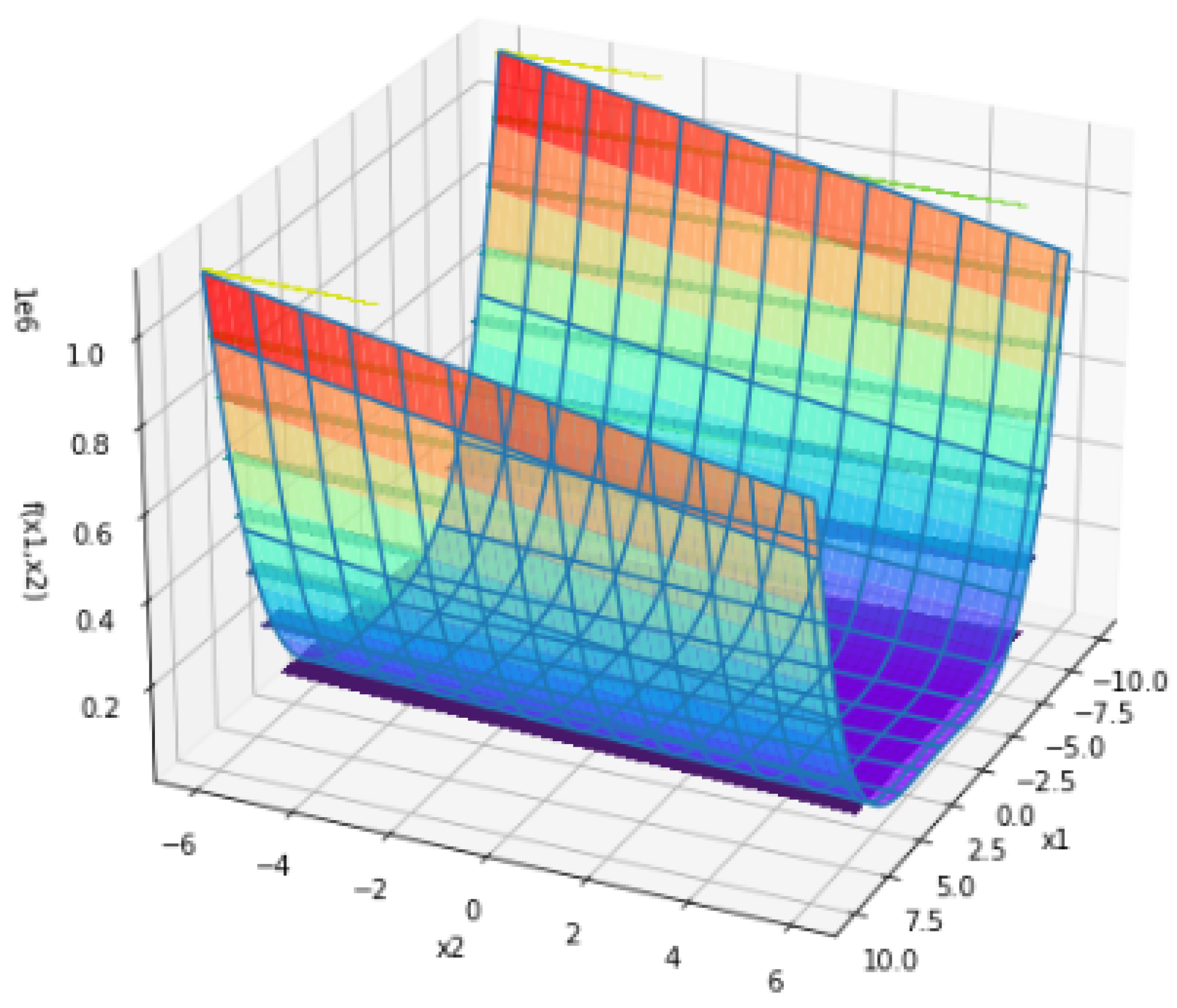
Example 1.
Consider the non-convex Rosenbrock function f : R 2 R such that
f ( x 1 , x 2 ) = 100 ( x 2 x 1 2 ) 2 + ( x 1 1 ) 2 .
Following Figure 1 represents the surface plot of the Rosenbrock function:
The Rosenbrock function was introduced by Rosenbrock in 1960. We tested modified q-BFGS, q-BFGS, and BFGS algorithms for 10 different initial points. Numerical results for the Rosenbrock function are given in the following Table 1:
The Rosenbrock function converges to x * = ( 1 , 1 ) T with value f ( x * ) = 0 , for the above starting points x 0 . Figure 2, Figure 3, and Figure 4 show the Dolan and More performance profiles of modified q-BFGS, q-BFGS, and BFGS algorithms for the Rosenbrock function, respectively.
The global minima and plotting points of the Rosenbrock function using the modified q-BFGS algorithm can also be observed in Figure 5.
For the starting point x 0 = ( 1.5 , 1 ) , the Rosenbrock function converges to
x * = [ 0.999999996685342 , 0.999999997414745 ] T , with f ( x * ) = 1.64642951315324 e 15 and q f ( x * ) = [ 1.66435354 e 06 , 7.98812111 e 07 ] T ,
in 25 iterations.
The global minima and plotting points of the Rosenbrock function using the q-BFGS algorithm can also be observed in Figure 6.
For the starting point x 0 = ( 1.5 , 1 ) , the Rosenbrock function converges to
x * = [ 1.0000000 , 1.00000001 ] T , with f ( x * ) = 1.541354346404984 e 16 and q f ( x * ) = [ 4.42018890 e 07 , 2.47425057 e 07 ] T .
in 47 iterations.
The global minima and plotting points of the Rosenbrock function using the BFGS algorithm can also be observed in Figure 7.
For the starting point x 0 = ( 1.5 , 1 ) , the Rosenbrock function converges to
x * = [ 0.99999552 , 0.99999103 ] T , with f ( x * ) = 2.0060569721431806 e 11 and q f ( x * ) = [ 7.91549092 e 07 , 3.95920563 e 07 ] T ,
in 49 iterations.
Example 2.
We consider
f ( x ) = x 2 2 if x < 2 x 2 + 2 if x 2 ,
which is non-differentiable at x = 2 . For initial point x 0 = 9 , using our modified q-BFGS algorithm we reach minima at x * = 0 in 4 iterations, 10 function evaluations, and 5 gradient evaluations.
Example 3.
Consider the non-convex Rastrigin function f such that
f ( x ) = 10 d + i = 1 d [ x i 2 10 c o s ( 2 π x i ) ]
Following Figure 8 represents the surface plot of the Rastrigin function:
The Rastrigin function f has a global minimum at
x * = ( 0 , 0 , , 0 ) ,
with value
f ( x * ) = 0 .
We tested modified q-BFGS, q-BFGS, and, BFGS algorithms for initial point x 0 = ( 0.2 , 0.2 ) .
The global minima and plotting points of the Rastrigin function using the modified q-BFGS algorithm can be observed in Figure 9.
The numerical results for the Rastrigin function, using the modified q-BFGS algorithm are as follows:
For the starting point x 0 = ( 0.2 , 0.2 ) , the Rastrigin function converges to
x * = [ 6.83810097023008 e 6 , 6.83810097023008 e 6 ] T , with f ( x * ) = 1.85534789132191 e 9 and q f ( x * ) = [ 1.3676 e 6 , 1.3676 e 6 ] T .
NI/NF/NG = 4 / 18 / 6 .
The global minima and plotting points of the Rastrigin function using the q-BFGS algorithm can be observed in Figure 10.
The numerical results for the Rastrigin function, using the q-BFGS algorithm are as follows:
For the starting point x 0 = ( 0.2 , 0.2 ) , The Rastrigin function converges to
x * = [ 1.18906228 e 06 , 2.65293229 e 07 ] T , with f ( x * ) = 2.944648969105401 e 10 and q f ( x * ) = [ 0 . , 0 . ] T .
NI/NF/NG = 5 / 24 / 8 .
The global minima and plotting points of the Rastrigin function using the BFGS algorithm can be observed in Figure 11.
The numerical results for the Rastrigin function using the BFGS algorithm are as follows:
For the starting point x 0 = ( 0.2 , 0.2 ) , the Rastrigin function converges to
x * = ( 7.14289963 e 09 , 7.37267609 e 09 ) T , with f ( x * ) = 2.1316282072803006 e 14 and f ( x * ) = ( 1.1920929 e 07 , 0.0000000 e 00 ) T .
NI/NF/NG = 7 / 36 / 12 .
From the above numerical results, we conclude that using the modified q-BFGS algorithm, we can reach the critical point by taking the least number of iterations.
Example 4.
Consider the SIX-HUMP CAMEL function f : R 2 R such that
f ( x ) = 4 2.1 x 1 2 + x 1 4 3 x 1 2 + x 1 x 2 + ( 4 + 4 x 2 2 ) x 2 2
The Figure 12 on the left shows the SIX-HUMP CAMEL function on its recommended input domain and on the right shows only a portion of this domain for easier view of the function’s key characteristics. The function f has six local minima, two of which are global.
Input Domain: The function is usually evaluated on the rectangle x 1 [ 3 , 3 ] , x 2 [ 2 , 2 ] .
This function has a global minimum at
x * = ( 0.0898 , 0.7126 ) and ( 0.0898 , 0.7126 ) ,
with value
f ( x * ) = 1.0316 .
For the starting point x 0 = ( 1 , 1 ) , with the modified q-BFGS algorithm f converges to x * in eight iterations whereas with q-BFGS and BFGS it takes 13 iterations. Table 2, Table 3, and Table 4 give numerical results and Figure 13, Figure 14, and Figure 15 represents the global minima and sequence of iterative points generated with modified q-BFGS, q-BFGS and BFGS algorithms, respectively.
Table 2. Numerical results for Modified q-BFGS algorithm.
S.N.x f ( x ) q f ( x )
1 ( 1 , 1 ) T 3.23333333333333 ( 2.59999999 , 8.9999998 ) T
2 ( 0.675 , 0.12499997 ) T 1.27218227259399 ( 2.97185835 , 1.64374981 ) T
3 ( 0.06796459 , 0.53593743 ) T −0.764057148938559 ( 1.0770199 , 1.75654714 ) T
4 ( 0.0353348602 , 0.8064736058 ) T −0.876032180235736 ( 1.08878201 , 1.97602868 ) T
5 ( 0.117691114989 , 0.69297924267 ) T −1.02498975962408 ( 0.23490147 , 0.33700269 ) T
6 ( 0.087916835437 , 0.709453427634 ) T −1.03153652682667 ( 0.01181639 , 0.05018343 ) T
7 ( 0.089782273326 , 0.71271422021 ) T −1.03162840874522 ( 0.00052364 , 0.00100674 ) T
8 ( 0.089842117966 , 0.71265601378 ) T −1.03162845348855 ( 1.20226364 × 10 6 , 6.54303983 × 10 6 ) T
Here, we obtain x * = ( 0.089842117966 , 0.71265601378 ) T
f ( x * ) = 1.03162845348988 and q f ( x * ) = ( 6.20473783 × 10 09 , 0.00000000 × 10 + 00 ) T
Figure 13. Global minima of SIX-HUMP CAMEL function using modified q-BFGS algorithm.
Mathematics 11 01420 g013
Table 3. Numerical results for q-BFGS algorithm [34].
S.N.x f ( x ) q f ( x )
1 ( 1 , 1 ) T 3.23333333333333 ( 2.59999999 , 8.9999998 ) T
2 ( 0.71968495 , 0.02967868 ) T 1.57257718494530 ( 3.04212661 , 0.4826738 ) T
3 ( 0.36642555 , 0.07524058 ) T 0.505072874807150 ( 2.60658417 , 0.22868392 ) T
4 ( 0.13008033 , 0.06568514 ) T 0.0413558838831559 ( 0.95654292 , 0.65102699 ) T
5 ( 0.00245036 , 0.12816569 ) T −0.0649165012454617 ( 0.10856293 , 0.99409097 ) T
6 ( 0.11507302 , 0.35694646 ) T −0.351034437749229 ( 1.26477125 , 2.01283747 ) T
7 ( 0.23737914 , 0.62081297 ) T −0.581320173229039 ( 2.40899478 , 0.90085665 ) T
8 ( 0.08148802 , 0.6924283 ) T −0.915418626192531 ( 1.33979439 , 0.14610549 ) T
9 ( 0.11917819 , 0.6987523 ) T −1.02633316281778 ( 0.24050227 , 0.25049034 ) T
10 ( 0.0912121 , 0.72252832 ) T −1.03082558867975 ( 0.00080671 , 0.16366308 ) T
11 ( 0.087625 , 0.71111103 ) T −1.03159319420704 ( 0.01575222 , 0.02301181 ) T
12 ( 0.09005303 , 0.71260578 ) T −1.03162824822151 ( 0.00169591 , 0.00104015 ) T
13 ( 0.08983369 , 0.71266332 ) T −1.03162845277086 ( 7.18180083 × 10 5 , 1.21481195 × 10 4 ) T
Here, we obtain x * = ( 0.08983369 , 0.71266332 ) T ,
f ( x * ) = 1.0316284534898477 and q f ( x * ) = ( 0.00000000 × 10 + 00 , 9.65876859 × 10 07 ) T .
Using this q-BFGS algorithm, we can reach the critical point by taking 13 iterations.
Figure 14. Global minima of SIX-HUMP CAMEL function using q-BFGS algorithm.
Mathematics 11 01420 g014
Table 4. Numerical results for BFGS algorithm.
S.N.x f ( x ) q f ( x )
1 ( 1 , 1 ) T 3.23333333333333 ( 2.59999999 , 8.9999998 ) T
2 ( 0.71968497 , 0.02967869 ) T 1.5725772653791203 ( 3.04212611 , 0.48267368 ) T
3 ( 0.13008034 , 0.06568512 ) T 0.041355907444434827 ( 0.95654306 , 0.65102689 ) T
4 ( 0.00245035 , 0.12816566 ) T −0.06491646830150141 ( 0.10856298 , 0.99409077 ) T
5 ( 0.11507301 , 0.35694647 ) T −0.35103445558228663 ( 1.26477118 , 2.01283762 ) T
6 ( 0.23737911 , 0.62081301 ) T −0.5813202779118049 ( 2.40899456 , 0.90085617 ) T
7 ( 0.08148803 , 0.6924282 ) T −0.9154186025665918 ( 1.33979439 , 0.1461069 ) T
8 ( 0.11917811 , 0.69875236 ) T −1.0263331977999757 ( 0.24050162 , 0.25048941 ) T
9 ( 0.09121207 , 0.72252828 ) T −1.0308255945761227 ( 0.00080669 , 0.16366242 ) T
10 ( 0.08762501 , 0.71111104 ) T −1.031593194593363 ( 0.01575207 , 0.02301181 ) T
11 ( 0.09005304 , 0.71260578 ) T −1.031628248214576 ( 0.00169598 , 0.00104006 ) T
12 ( 0.08983368 , 0.7126633 ) T −1.0316284527721356 ( 0.000016959 , 0.000104006 ) T
13 ( 0.08984197 , 0.71265633 ) T −1.0316284534898297 ( 7.19424520 × 10 5 , 1.21236354 × 10 4 ) T
Here, we obtain x * = ( 0.08984197 , 0.71265633 ) T ,
f ( x * ) = 1.0316284534898448 and f ( x * ) = ( 2.68220901 × 10 07 , 9.98377800 × 10 07 ) T .
Using this BFGS algorithm, we can reach the critical point by taking 13 iterations.
Figure 15. Global minima of SIX-HUMP CAMEL function using BFGS algorithm.
Mathematics 11 01420 g015
We conclude that using the modified q-BFGS algorithm, we can reach the critical point by taking the least number of iterations. From the performance results and plotting points for the multimodal functions it could be seen that the q-descent direction has a mechanism to escape from many local minima and move towards the global minimum.
Now, we compare the performance of numerical algorithms for large dimensional Rosenbrock and Wood function. Numerical results for these functions are given in Table 5 and Table 6.
Numerical results for the large dimensional Rosenbrock function for x 0 = ( 0 , 0 , , 0 )
f ( x ) = i = 1 d 1 [ 100 ( x i + 1 x i 2 ) 2 + ( x i 1 ) 2 ]
Table 5. Comparison of numerical results of Modified q-BFGS, q-BFGS, and BFGS algorithm for the large dimensional Rosenbrock function.
S.No.DimensionModified q-BFGSq-BFGSBFGS
NI/NF/NGNI/NF/NGNI/NF/NG
11058/889/13263/972/8161/1365/123
250242/15,432/300253/17,316/324253/17,199/337
3100466/63,088/604486/64,056/636479/64,741/641
4200904/209,912/1175978/248,056/1228956/253,674/1262
Numerical results for large dimensional WOOD function [39] for x 0 = ( 0 , 0 , , 0 )
Table 6. Comparison of numerical results of Modified q-BFGS, q-BFGS, and BFGS algorithm for Large Dimensional Wood function.
S.No.DimensionModified q-BFGSq-BFGSBFGS
NI/NF/NGNI/NF/NGNI/NF/NG
12085/1976/9891/2872/130103/2478/118
280162/19,745/198193/21,250/259209/22,366/276
3100197/19,965/255240/30,714/301254/29,290/290
4200296/75,686/397370/93,538/463378/93,678/466
We have taken 20 test problems to show the proposed method’s efficiency and numerical results. We take tolerance ϵ = 10 6 , σ 1 = 0.0001 , and σ 2 = 0.9 . Our numerical results are shown in Table 7, Table 8 and Table 9 with the problem number(S.N.), problem name, Dimension (DIM), starting point, the total number of iterations (NI), the total number of function evaluations (NF), the total number of gradient evaluations (NG), respectively.
Table 5, Table 6, Table 7, Table 8 and Table 9 show that the modified q-BFGS algorithm solves about 86% of the test problems with the least number of iterations, 82% of the test problems with the least number of function evaluations, and 52% of the test problems with the least number of gradient evaluations. Therefore, with Figure 16, Figure 17 and Figure 18 we conclude that the modified q-BFGS performs better than other algorithms and improves the performance in fewer iterations, function evaluations, and gradient evaluations.
In Figure 17 and Figure 18 the graph of q-BFGS and BFGS method does not converge to 1 as the methods fail to minimize two problems for each as given in Table 8 and Table 9.

6. Conclusions and Future Directions

We have given a new q-quasi-Newton equation and proposed a modified q-BFGS method for unconstrained minimization based on this new q-quasi-Newton equation. The method converges globally with a q-gradient-based Armijo–Wolfe line search. The q-gradient allows the search direction to be taken from a diverse set of directions and takes large steps to converge. From the performance results and plotting points for the multimodal functions, it could be seen that the q-descent direction and q-gradient-based line search have a mechanism to escape from many local minima and move towards the global minimum. The first order q-differentiability of the function is sufficient to prove the global convergence of the proposed method. The convergence and numerical results show that the algorithm given in this paper is very successful. However, many other q-quasi-Newton methods still need to be studied using the q-derivative.

Author Contributions

Formal analysis, K.K.L., S.K.M., R.S., M.S. and B.R.; funding acquisition, K.K.L.; investigation, S.K.M.; methodology, S.K.M., R.S., M.S. and B.R.; supervision, S.K.M.; validation, R.S.; writing—original draft, R.S.; writing—review and editing, K.K.L., R.S., M.S. and B.R. All authors have read and agreed to the published version of the manuscript.

Funding

The Second author is financially supported by Research Grant for Faculty (IoE Scheme) under Dev. Scheme No. 6031 and the third author is financially supported by the BHU-UGC Non-NET fellowship /R/Dev./ix-Sch.(BHU Res.Sch.)/2022-23/46476. The fifth author is financially supported by the Centre for Digital Transformation, Indian Institute of Management, Ahmedabad.

Institutional Review Board Statement

Not applicable.

Informed Consent Statement

Not applicable.

Data Availability Statement

No data were used to support this study.

Acknowledgments

The authors are indebted to the anonymous reviewers for their valuable comments and remarks that helped to improve the presentation and quality of the manuscript.

Conflicts of Interest

The authors declare no conflict of interest.

References

  1. Mishra, S.K.; Ram, B. Conjugate gradient methods. In Introduction to Unconstrained Optimization with R; Springer Nature: Singapore, 2019; pp. 211–244. [Google Scholar]
  2. Fletcher, R. Practical Methods of Optimization; John Wiley & Sons: Chichester, NY, USA, 2013. [Google Scholar]
  3. Gill, P.; Murray, W.; Wright, M. Practical Optimization; Academic Press: Cambridge, MA, USA, 1981. [Google Scholar]
  4. Mishra, S.K.; Ram, B. Newton’s method. In Introduction to Unconstrained Optimization with R; Springer Nature: Singapore, 2019; pp. 175–209. [Google Scholar]
  5. Mishra, S.K.; Ram, B. Quasi-Newton methods. In Introduction to Unconstrained Optimization with R; Springer Nature: Singapore, 2019; pp. 245–289. [Google Scholar]
  6. Fletcher, R. A new approach to variable metric algorithms. Comput. J. 1970, 13, 317–322. [Google Scholar] [CrossRef] [Green Version]
  7. Goldfarb, D. A family of variable-metric methods derived by variational means. Math. Comput. 1970, 24, 23–26. [Google Scholar] [CrossRef]
  8. Shanno, D.F. Conditioning of quasi-Newton methods for function minimization. Math. Comput. 1970, 24, 647–656. [Google Scholar] [CrossRef]
  9. Broyden, C.G. The convergence of a class of double-rank minimization algorithms: 2. The new algorithm. IMA J. Appl. Math. 1970, 6, 222–231. [Google Scholar] [CrossRef] [Green Version]
  10. Mascarenhas, W.F. The BFGS method with exact line searches fails for non-convex objective functions. Math. Program. 2004, 99, 49. [Google Scholar] [CrossRef]
  11. Li, D.H.; Fukushima, M. On the global convergence of the BFGS method for nonconvex unconstrained optimization problems. SIAM J. Optim. 2001, 11, 1054–1064. [Google Scholar] [CrossRef] [Green Version]
  12. Li, D.; Fukushima, M. A globally and superlinearly convergent gauss–Newton-based BFGS method for symmetric nonlinear equations. SIAM J. Numer. Anal. 1999, 37, 152–172. [Google Scholar] [CrossRef]
  13. Kac, V.G.; Cheung, P. Quantum Calculus; Springer: Berlin, Germany, 2002; Volume 113. [Google Scholar]
  14. Ernst, T. A Comprehensive Treatment of q-Calculus; Springer: Basel, Switzerland, 2012. [Google Scholar]
  15. Cieśliński, J.L. Improved q-exponential and q-trigonometric functions. Appl. Math. Lett. 2011, 24, 2110–2114. [Google Scholar] [CrossRef]
  16. Borges, E.P. A possible deformed algebra and calculus inspired in nonextensive thermostatistics. Phys. A Stat. Mech. Its Appl. 2004, 340, 95–101. [Google Scholar] [CrossRef] [Green Version]
  17. Tariboon, J.; Ntouyas, S.K. Quantum calculus on finite intervals and applications to impulsive difference equations. Adv. Differ. Equations 2013, 2013, 282. [Google Scholar] [CrossRef] [Green Version]
  18. Jackson, F.H. XI.—On q-functions and a certain difference operator. Earth Environ. Sci. Trans. R. Soc. Edinb. 1909, 46, 253–281. [Google Scholar] [CrossRef]
  19. Rajković, P.; Stanković, M.; Marinković, D.S. Mean value theorems in g-calculus. Mat. Vesn. 2002, 54, 171–178. [Google Scholar]
  20. Ismail, M.E.; Stanton, D. Applications of q-Taylor theorems. J. Comput. Appl. Math. 2003, 153, 259–272. [Google Scholar] [CrossRef] [Green Version]
  21. Jing, S.C.; Fan, H.Y. q-Taylor’s Formula with Its q-Remainder1. Commun. Theor. Phys. 1995, 23, 117. [Google Scholar] [CrossRef]
  22. Rajković, P.M.; Marinković, S.D.; Stanković, M.S. Fractional integrals and derivatives in q-calculus. Appl. Anal. Disc. Math. 2007, 1, 311–323. [Google Scholar]
  23. Jackson, D.O.; Fukuda, T.; Dunn, O.; Majors, E. On q-definite integrals. Q. J. Pure Appl. Math. 1910, 41, 193–203. [Google Scholar]
  24. Soterroni, A.C.; Galski, R.L.; Ramos, F.M. The q-gradient vector for unconstrained continuous optimization problems. In Operations Research Proceedings 2010; Springer: Heidelberg, Germany, 2011; pp. 365–370. [Google Scholar]
  25. Gouvêa, É.J.; Regis, R.G.; Soterroni, A.C.; Scarabello, M.C.; Ramos, F.M. Global optimization using q-gradients. Eur. J. Oper. Res. 2016, 251, 727–738. [Google Scholar] [CrossRef]
  26. Lai, K.K.; Mishra, S.K.; Ram, B. On q-quasi-Newton’s method for unconstrained multiobjective optimization problems. Mathematics 2020, 8, 616. [Google Scholar] [CrossRef] [Green Version]
  27. Mishra, S.K.; Samei, M.E.; Chakraborty, S.K.; Ram, B. On q-variant of Dai–Yuan conjugate gradient algorithm for unconstrained optimization problems. Nonlinear Dyn. 2021, 104, 2471–2496. [Google Scholar] [CrossRef]
  28. Lai, K.K.; Mishra, S.K.; Ram, B. A q-conjugate gradient algorithm for unconstrained optimization problems. Pac. J. Optim 2021, 17, 57–76. [Google Scholar]
  29. Van Voorhis, T.; Head-Gordon, M. A geometric approach to direct minimization. Mol. Phys. 2002, 100, 1713–1721. [Google Scholar] [CrossRef]
  30. [yop] Dominic, S.; Shardt, Y.; Ding, S. Economic performance indicator based optimization for the air separation unit compressor trains. IFAC-PapersOnLine 2015, 48, 858–863. [Google Scholar] [CrossRef]
  31. Dutta, S. Optimization in Chemical Engineering; Cambridge University Press: Cambridge, UK, 2016. [Google Scholar]
  32. Head, J.D.; Zerner, M.C. A Broyden—Fletcher—Goldfarb—Shanno optimization procedure for molecular geometries. Chem. Phys. Lett. 1985, 122, 264–270. [Google Scholar] [CrossRef]
  33. Ahuja, K.; Green, W.H.; Li, Y.P. Learning to optimize molecular geometries using reinforcement learning. J. Chem. Theory Comput. 2021, 17, 818–825. [Google Scholar] [CrossRef]
  34. Mishra, S.K.; Panda, G.; Chakraborty, S.K.; Samei, M.E.; Ram, B. On q-BFGS algorithm for unconstrained optimization problems. Adv. Differ. Equ. 2020, 2020, 638. [Google Scholar] [CrossRef]
  35. Wei, Z.; Li, G.; Qi, L. New quasi-Newton methods for unconstrained optimization problems. Appl. Math. Comput. 2006, 175, 1156–1188. [Google Scholar] [CrossRef]
  36. Yuan, Y. A modified BFGS algorithm for unconstrained optimization. IMA J. Numer. Anal. 1991, 11, 325–332. [Google Scholar] [CrossRef]
  37. Deng, N.; Li, Z. Some global convergence properties of a conic-variable metric algorithm for minimization with inexact line searches. Optim. Methods Softw. 1995, 5, 105–122. [Google Scholar] [CrossRef]
  38. Li, D.H.; Fukushima, M. A modified BFGS method and its global convergence in nonconvex minimization. J. Comput. Appl. Math. 2001, 129, 15–35. [Google Scholar] [CrossRef] [Green Version]
  39. Moré, J.J.; Garbow, B.S.; Hillstrom, K.E. Testing unconstrained optimization software. ACM Trans. Math. Softw. (TOMS) 1981, 7, 17–41. [Google Scholar] [CrossRef] [Green Version]
  40. Dolan, E.D.; Moré, J.J. Benchmarking optimization software with performance profiles. Math. Program. 2002, 91, 201–213. [Google Scholar] [CrossRef]
Figure 1. Surface plot of Rosenbrock function.
Mathematics 11 01420 g001
Figure 2. Performance profile based on number of iterations.
Mathematics 11 01420 g002
Figure 3. Performance profile based on number of gradient evaluations.
Mathematics 11 01420 g003
Figure 4. Performance profile based on number of function evaluations.
Mathematics 11 01420 g004
Figure 5. Global minima of the Rosenbrock function using modified q-BFGS algorithm.
Mathematics 11 01420 g005
Figure 6. Global minima of the Rosenbrock function using q-BFGS algorithm [34].
Mathematics 11 01420 g006
Figure 7. Global minima of the Rosenbrock function using BFGS algorithm.
Mathematics 11 01420 g007
Figure 8. Surface plot of the Rastrigin function.
Mathematics 11 01420 g008
Figure 9. Global minima of the Rastrigin function using the modified q-BFGS algorithm.
Mathematics 11 01420 g009
Figure 10. Global minima of the Rastrigin function using q-BFGS algorithm.
Mathematics 11 01420 g010
Figure 11. Global minima of the Rastrigin function using BFGS algorithm.
Mathematics 11 01420 g011
Figure 12. Surface plot of the SIX-HUMP CAMEL function.
Mathematics 11 01420 g012
Figure 16. Performance Profile based on number of iterations.
Mathematics 11 01420 g016
Figure 17. Performance Profile based on number of function evaluations.
Mathematics 11 01420 g017
Figure 18. Performance Profile based on number of gradient evaluations.
Mathematics 11 01420 g018
Table 1. Comparison of numerical results of Modified q-BFGS, q-BFGS, and BFGS algorithms for the Rosenbrock function.
S.No. x 0 Modified q-BFGSq-BFGSBFGS
NI/NF/NGNI/NF/NGNI/NF/NG
1 ( 1.5 , 1 ) T 25/95/4747/198/6649/213/71
2 ( 0 , 0 ) T 22/77/3521/78/2620/75/25
3 ( 4 , 4 ) T 27/125/7363/82/24663/255/85
4 ( 3 , 0 ) T 28/118/6455/210/7058/210/70
5 ( 10 , 0 ) T 54/197/9140/150/5085/372/120
6 ( 7 , 7 ) T 52/184/8275/294/9876/414/134
7 ( 4 , 5 ) T 48/174/8051/201/6751/198/66
8 ( 2 , 2 ) T 26/112/6255/201/6757/342/110
9 ( 1 , 1.2 ) T 9/38/2213/57/1912/93/27
10 ( 0 , 4 ) T 27/113/6125/96/3226/114/38
Table 7. Numerical results for Modified q-BFGS algorithm.
S.N.Problems x 0 DIMNINFNG x *
1ROSENBROCK ( 1.5 , 1 ) T 2259547 ( 1.0000 , 1.0000 ) T
2FROTH ( 0.5 , 2 ) T 293720 ( 11.4128 , 0.8968 ) T
3BADSCP ( 0 , 1 ) T 2174618272 ( 1.0981 × 10 5 , 9.1062 ) T
4BADSCB ( 1 , 1 ) T 21110080 ( 1000000.0000 , 1.9999 × 10 6 ) T
5BEALE ( 3 , 1 ) T 2124421 ( 3.0000 , 0.5000 ) T
6JENSAM ( 1 , 0.4 ) T 2155720 ( 0.56094 , 0.56094 ) T
7WOOD ( 3 , 1 , 3 , 1 ) T 44220552 ( 1.0000 , 1.0000 , 1.0000 , 1.0000 ) T
8POWELL SINGULAR ( 3 , 1 , 0 , 1 ) T 4239146 ( 0.0011 , 0.0001 , 0.0009 , 0.0009 ) T
9RASTRIGIN ( 0.2 , 0.2 ) T 24186 ( 6.8381 × 10 5 , 6.8381 × 10 5 ) T
10GOLDSTEIN PRICE ( 0.5 , 0.5 ) T 21210684 ( 5.4911 × 10 5 , 1.0000 ) T
11THREE-HUMP CAMEL ( 2.5 , 0 ) T 251910 ( 8.3463 × 10 8 , 1.9707 × 10 7 ) T
12COLVILLE ( 0 , 0 , 0 , 0 ) T 42710956 ( 1.0000 , 1.0000 , 1.0000 , 1.0000 ) T
13BOOTH ( 2 , 2 ) T 22118 ( 1.0000 , 3.0000 ) T
14SINE VALLEY ( 3 π / 2 , 1 ) T 23511546 ( 1.4495 × 10 11 , 1.6686 × 10 11 ) T
15BRANIN ( 9.3 , 3 ) T 25189 ( 9.4248 , 2.4750 ) T
16SIX HUMP CAMEL ( 1 , 1 ) T 283217 ( 0.0898 , 0.7126 ) T
17HIMMELBLAU ( 1 , 1 ) T 293720 ( 3.0000 , 2.0000 ) T
18SHEKEL ( 0 , 0 , 0 , 0 ) T 41410535 ( 4.0007 , 4.0005 , 3.9997 , 3.9995 ) T
19HARTMAN 3D ( 0 , 0.5 , 0.4 ) T 31010021 ( 0.1146 , 0.5556 , 0.8525 ) T
20GRIEWANK ( 2 , 1.2 ) T 28259 ( 6.9305 × 10 5 , 5.0749 × 10 5 ) T
Table 8. Numerical results for q-BFGS algorithm.
S.N.Problems x 0 DIMNINFNG x *
1ROSENBROCK ( 1.5 , 1 ) T 24719866 ( 1.0000 , 1 . 0000 T
2FROTH ( 0.5 , 2 ) T 293010 ( 11.4127 , 0.8968 ) T
3BADSCP ( 0 , 1 ) T 2158609203 ( 1.0981 × 10 5 , 9.1061 ) T
4BADSCB ( 1 , 1 ) T 2----
5BEALE ( 3 , 1 ) T 2134816 ( 3.0000 , 0.5000 ) T
6JENSAM ( 1 , 0.4 ) T 2176622 ( 0.56095 , 0.56095 ) T
7WOOD ( 3 , 1 , 3 , 1 ) T 487309103 ( 1.0000 , 1.0000 , 1.0000 , 1.0000 ) T
8POWELL SINGULAR ( 3 , 1 , 0 , 1 ) T 43712642 ( 2.3008 × 10 4 , 2.3007 × 10 5 , 9.0539 × 10 4 , 9.0545 × 10 4 ) T
9RASTRIGIN ( 0.2 , 0.2 ) T 25248 ( 1.1890 × 10 6 , 2.6529 × 10 7 ) T
10GOLDSTEIN PRICE ( 0.5 , 0.5 ) T 2----
11THREE-HUMP CAMEL ( 2.5 , 0 ) T 283612 ( 1.7475 , 0.8738 ) T
12COLVILLE ( 0 , 0 , 0 , 0 ) T 42610234 ( 1.0000 , 1.0000 , 1.0000 , 1.0000 ) T
13BOOTH ( 2 , 2 ) T 23155 ( 1.0000 , 3.0000 ) T
14SINE VALLEY ( 3 π / 2 , 1 ) T 23713244 ( 4.0788 × 10 10 , 4.262 × 10 10 ) T
15BRANIN ( 9.3 , 3 ) T 26248 ( 9.4248 , 2.4750 ) T
16SIX HUMP CAMEL ( 1 , 1 ) T 2135418 ( 0.0898 , 0.7126 ) T
17HIMMELBLAU ( 1 , 1 ) T 283913 ( 3.0000 , 2.0000 ) T
18SHEKEL ( 0 , 0 , 0 , 0 ) T 41410535 ( 4.0007 , 4.0006 , 3.9997 , 3.9995 ) T
19HARTMAN 3D ( 0 , 0.5 , 0.4 ) T 3116321 ( 0.1088 , 0.5556 , 0.8526 ) T
20GRIEWANK ( 2 , 1.2 ) T 28279 ( 8.4001 × 10 5 , 3.1323 × 10 4 ) T
Table 9. Numerical results for BFGS algorithm.
S.N.Problems x 0 DIMNINFNG x *
1ROSENBROCK ( 1.5 , 1 ) T 24921371 ( 1.0000 , 1 . 0000 T
2FROTH ( 0.5 , 2 ) T 293010 ( 11.4128 , 0.8968 ) T
3BADSCP ( 0 , 1 ) T 2----
4BADSCB ( 1 , 1 ) T 2----
5BEALE ( 3 , 1 ) T 2134816 ( 3.0000 , 0.5000 ) T
6JENSAM ( 1 , 0.4 ) T 2176622 ( 0.56095 , 0.56095 ) T
7WOOD ( 3 , 1 , 3 , 1 ) T 489525105 ( 1.0000 , 1.0000 , 1.0000 , 1.0000 ) T
8POWELL SINGULAR ( 3 , 1 , 0 , 1 ) T 44123046 ( 7.759 × 10 4 , 7.7607 × 10 5 , 7.5812 × 10 4 , 7.581 × 10 4 ) T
9RASTRIGIN ( 0.2 , 0.2 ) T 273612 ( 7.1429 × 10 9 , 7.3727 × 10 7 ) T
10GOLDSTEIN PRICE ( 0.5 , 0.5 ) T 2177525 ( 9.9828 × 10 9 , 1.0000 ) T
11THREE-HUMP CAMEL ( 2.5 , 0 ) T 283612 ( 1.7475 , 0.8738 ) T
12COLVILLE ( 0 , 0 , 0 , 0 ) T 43119038 ( 1.0000 , 1.0000 , 1.0000 , 1.0000 ) T
13BOOTH ( 2 , 2 ) T 23155 ( 1.0000 , 3.0000 ) T
14SINE VALLEY ( 3 π / 2 , 1 ) T 23714147 ( 5.9619 × 10 6 , 5.9674 × 10 6 ) T
15BRANIN ( 9.3 , 3 ) T 26248 ( 9.4248 , 2.4750 ) T
16SIX HUMP CAMEL ( 1 , 1 ) T 2135418 ( 0.0898 , 0.7126 ) T
17HIMMELBLAU ( 1 , 1 ) T 283913 ( 3.0000 , 2.0000 ) T
18SHEKEL ( 0 , 0 , 0 , 0 ) T 41216032 ( 4.0007 , 4.0006 , 3.9997 , 3.9995 ) T
19HARTMAN 3D ( 0 , 0.5 , 0.4 ) T 3148020 ( 0.1146 , 0.5556 , 0.8525 ) T
20GRIEWANK ( 2 , 1.2 ) T 2103311 ( 6.872 × 10 8 , 7.2441 × 10 4 ) T
Disclaimer/Publisher’s Note: The statements, opinions and data contained in all publications are solely those of the individual author(s) and contributor(s) and not of MDPI and/or the editor(s). MDPI and/or the editor(s) disclaim responsibility for any injury to people or property resulting from any ideas, methods, instructions or products referred to in the content.

