Abstract
Inhomogeneous random graphs are commonly used models for complex networks where nodes have varying degrees of connectivity. Computing the degree distribution of such networks is a fundamental problem and has important applications in various fields. We define the inhomogeneous random graph as a random graph model where the edges are drawn independently and the probability of a link between any two vertices can be different for each node pair. In this paper, we present an exact and an approximation method to compute the degree distribution of inhomogeneous random graphs using the Poisson binomial distribution. The exact algorithm utilizes the DFT-CF method to compute the distribution of a Poisson binomial random variable. The approximation method uses the Poisson, binomial, and Gaussian distributions to approximate the Poisson binomial distribution.
Keywords:
inhomogeneous random graph; Poisson binomial distribution; degree distribution; DFT-CF method MSC:
05C80
1. Introduction
Random graphs are widely used to model complex systems such as social networks, biological networks, and the internet. The degree distribution is an important characteristic of a network, as it provides information about the connectivity of nodes in the network [1], and its shape determines many network phenomena, such as robustness [2,3,4] or spreading processes [5,6,7]. Inhomogeneous random graphs are a type of random graph where the nodes are not equally likely to be connected. Instead, the probability of two nodes being connected depends on their attributes or characteristics. Example applications of inhomogeneous random graphs are social network analysis [8,9], modelling biological networks [10], or modelling transportation networks [11].
In the literature of network science and random graphs, inhomogeneous random graphs are not a well-defined random graph model, but they are a family of random graph models, where the nodes have varying degrees of connectivity. One example for inhomogeneous random graphs is the stochastic block model [8,9]. A stochastic block model (SBM) is defined by a partition of the vertex set and a symmetric P edge probability matrix. For any two vertices and , the draw probability of the undirected edge is . Therefore, for any vertex pair, the probability that the nodes u and v are connected is directly determined by the model parameters (the P matrix), and the links are drawn independently if the P matrix is given. A second example is the generalized random graph [12,13]. In case of a generalized random graph (GRG), the inhomogeneity is introduced into the model using vertex weights. For any i node of the network, there is given a vertex weight, and the probability that a edge is drawn between the nodes i and j is equal to
where is the total weight of all vertices. The consequence of this definition is that vertices with high weight are more likely to have many neighbours than vertices with small weights, and vertices with extremely high weights could act as hubs observed in many real-world networks. Furthermore, if the parameters are deterministic and given, the edge probabilities can be computed with (1), and the edges are independent. A third example for inhomogeneous random graphs is the biased static edge voting model [14]. We use this model in our numerical tests in Section 4, and it is briefly described in Section 4.2. Similarly to the SBM and GRG models, if the model parameters are given, the link probability of any node pair can be directly computed (see Equation (66)), and the edges are drawn independently.
For all these example inhomogeneous random graph models, the common property is that the edge probabilities can be directly computed from the model definition, and the edges are drawn independently. We define the inhomogeneous random graph (IRG) model via these properties (as it is defined in [13] (Section 6.7)). The inhomogeneous random graph is a random graph model on the vertex set , where the draw probability of any edge is given, and the edges are drawn independently. The IRG model can be considered as the natural generalization of the Erdős–Rényi (ER) random graph [15], where each link of the graph is drawn independently with a fixed p probability. If we set all the edge probabilities of the IRG model to a fixed p value, then we obtain an ER random graph. It is well known that the degree distribution of the ER model is close to the Poisson distribution [15]. When we observe the degree sequence of real-world networks, we often see that their empirical degree distribution has a fat tail [13]. Therefore, the ER random graph cannot be used to model real-world networks.
If the parameters are deterministic and given, the SBM, GRG, and the static edge voting model can be represented by an IRG. A further example for such a model is the Chung–Lu random graph [16]. However, not all inhomogeneous random graph models can be expressed as IRG. For example, the Norros–Reittu model [17] is a random multigraph model, while IRG is a model of a simple graph. A second example is the GRG model with random weights. Using random weights in GRG breaks the independence of the edges. A third example is the Barabási–Albert (BA) model [18]. The BA model is a dynamic network growth model, and for this case, we cannot derive the edge probabilities.
In this paper, we discuss a novel algorithm what allow us to compute the exact degree distribution of the IRG model and an approximation method to estimate the IRG degree distribution. The hardness of computing the degree distribution of the IRG model comes from the fact that each edge candidate of the network may have different draw probabilities; therefore, the degree distribution of any node is Poisson binomial (PB) [19,20]. The algorithm that we have developed to compute the degree distribution of the IRG model is based on the DFT-CF method invented by Yili Hong [19], and the approximation method uses the Poisson, binomial, and the Gaussian distributions to approximate the PB distribution. The proposed algorithms can be used to compute or approximate the degree distribution of any random graph model that can be represented by an IRG.
The structure of the remaining part of this paper is as follows: Section 2 contains the mathematical preliminaries of our study. In Section 2.1, we introduce the necessary notations and definitions. In Section 2.2, we briefly discuss the DFT-CF algorithm for computing the Poisson binomial distribution. Section 2.3 contains selected results about the approximation of the Poisson binomial distribution. In Section 3, we discuss the proposed algorithms to compute or approximate the degree distribution of the IRG model. In Section 3.1, we formally define the problem that we aim to solve. In Section 3.2, we present an exact algorithm to compute the degree distribution of the inhomogeneous random graph, and in Section 3.3, we discuss an approximation method to estimate this distribution. In the first part of Section 3.3, we outline the general scheme of the approximation method; then, we provide an upper bound of the approximation error for the special cases, when the approximator distribution is Poisson (Section 3.3.1), binomial (Section 3.3.2), and Gaussian (Section 3.3.3). The results of the numerical experiments are provided in Section 4. The study is concluded with the discussion in Section 5.
The contribution of the authors are a novel algorithm to compute the exact degree distribution of the IRG model utilizing the DFT-CF method (Section 3.2) and the analysis of the estimation method for this distribution (Section 3.3). The idea of the approximation scheme is simple and not new: we group the similar nodes into clusters and apply the same approximator distribution within a cluster. Our contribution here is the analysis of the approximation error in the specific cases when the approximator distribution is Poisson (Section 3.3.1), binomial (Section 3.3.2), and Gaussian (Section 3.3.3).
2. Preliminaries
2.1. Notations and Definitions
We denote the set as . A simple graph G is defined as a pair , where is the set of vertices and is the set of edges. The vertices are labeled with integers, so the vertex set of an n-vertex graph is . The degree of a vertex a is defined as the number of neighbors that a has in G. We denote the degree of a as or simply . The degree distribution of a deterministic or random graph G is defined as the distribution of , where U is a randomly and uniformly chosen vertex. Even in the case of a deterministic graph, is a random variable. In the deterministic case, we can express as . If G is a random graph, then is a random variable, and we refer to the distribution of as the degree distribution of vertex a.
The Poisson binomial random variable N is defined as the sum of n independent random indicators: , where , . Note that N takes value in . We say that the values are the parameters of the distribution, and we use the notation . When all s are identical, the distribution of N is binomial. Let , be the probability mass function (pmf) for the Poisson binomial random variable N. The pmf of N can be expressed as:
where is the set of all subsets of k integers that can be selected from , and is the complementary set of A in . The direct use of this formula is computationally very expensive.
We introduce now the inhomogeneous random graph (IRG) model [13] (Section 6.7), denoted by , where n is the number of vertices and is a set of edge probabilities. In this model, edges are drawn independently, and the probability of drawing the edge is given by for all . We formalize this as follows:
Definition 1.
The inhomogeneous random graph model is defined as a random graph with vertex set and edge probabilities , where each edge for all is drawn independently with probability .
The parameters of an IRG can also be represented by an symmetric P matrix with for all , and for any . Since the elements of the P matrix are probabilities, therefore, for all . By definition, the degree distribution of any i node in is Poisson binomial with the parameters .
We briefly introduce the discrete Fourier transformation (DFT). DFT transforms the sequence of complex numbers into another sequence of complex numbers , where the transformation is defined by the formula , , and . There are fast Fourier transform (FFT) algorithms to compute DFT efficiently. The best known and most commonly used FFT algorithm is the Cooley–Tukey algorithm [21].
We define the total variation norm [22,23] and, based on this, the total variational distance. Consider a signed measure on a measurable space . First, we define two non-negative measures:
The total variation norm of the measure is defined as:
The total variational distance of the probability measures P and Q on the same measurable space is defined as:
The factor 2 above is usually dropped. Informally, this is the largest possible difference between the probabilities that two probability measures can assign to the same event. For discrete probability distributions, it is possible to write the distance as follows, where the factor is applied to normalize to the range :
We continue with the definition of p-norm and p-distance. For any integer, the p-norm [24] of the function is defined as:
The distance [24] of the functions induced by the p-norm is given by:
We will use the notation to refer to the distribution of a random variable X.
2.2. Computing the Poisson Binomial Distribution: The DFT-CF Algorithm
Yili Hong showed in [19] that the probability mass function and the cumulative distribution function of the PB distribution can be computed directly using DFT. In particular, if , then for all :
where and . In other words:
Hong also provided an effective implementation of (11) in [19]. Let for all , where and are the real and imaginary parts of , respectively, and . It can be shown that , and for , the complex conjugate of can be expressed as:
Thus, and . Let , and denote the modulus and the argument of by and , respectively. Then, and can be explicitly expressed by . For all :
Here, and . The function is defined as:
According to this, we can use Algorithm 1 to compute the pdf of N, where denotes the ceiling function.
| Algorithm 1 Computing the Poisson binomial pdf |
| Let . |
| Let for , where: |
| return |
The derivation of (10) is based on the characteristic function and DFT; therefore, the method is called the DFT-CF algorithm.
2.3. Approximation of the Poisson Binomial Distribution
In this section, we discuss various approximations of the Poisson binomial distribution. We will use these results in Section 3.3 to derive upper bounds for the approximation error of the estimated IRG degree distribution. More information about approximating the PB distribution, as well as other results, can be found in the paper [20] by Wenpin Tang and Fengmin Tang.
2.3.1. Poisson Approximation
First, we consider the use of the Poisson distribution as an approximation of the PB distribution. We use the notation to the Poisson distribution with parameter . If X follows the PB distribution with parameters , then we can approximate the distribution of X by the Poisson distribution with the parameter . The following theorem shows us how well the Poisson distribution approximates the Poisson binomial distribution.
Theorem 1
([20,25]). Let and . Then
We see in [20] from (17) that the Poisson approximation of the PB distribution is good if , or equivalently, if . There are two cases:
- For small , the upper bound in (17) is sharp.
- For large , the approximation error is on the order of .
The constant in the lower bound can be improved to [26]. The Poisson approximation can be viewed as a mean-matching procedure.
In Section 3.3.1, we will use the following theorem to compute the total variation distance of two differently parametrized Poisson distribution functions:
Theorem 2
([27]). For any and :
2.3.2. Binomial Approximation
We denote the binomial distribution with parameters n and p by . Suppose that and . Then, we can use as an approximation of the distribution of X. The first result on the approximation precision of the Poission binomial distribution using the binomial distribution is due to Ehm [20,28]. The advantage of the binomial approximation over the Poisson approximation is justified by Theorem 3 from Choi and Xia:
Theorem 3
([20,29]). Let and . For , let . Then, for an m sufficiently large,
2.3.3. Gaussian Approximation
We denote the Gaussian distribution with expected value and variance by . The Gaussian approximation of the Poisson binomial distribution follows from the Lyapunov or Lindenberg central limit theorem [30]. If , and , then we can use the Gaussian distribution with the parameters and to approximate the distribution of X. The following theorem gives an upper bound for the error of Gaussian approximation in terms of p-distance:
Theorem 4
([20,31]). Let , and . Then there exists a universal constant such that
3. Materials and Methods
3.1. Problem Formulation
Suppose we are given an inhomogeneous random graph model (see Definition 1) with edge probabilities , . We aim to compute the degree distribution of . In particular, suppose that the node set of is , and U is a uniformly distributed random variable on the integers V. We are looking for the probabilities for all , where is the degree of node . In Section 3.2, we present an exact algorithm to compute , while in Section 3.3, we discuss an approximation method to estimate the values of .
3.2. Computing the Degree Distribution of Inhomogeneous Random Graph
We can apply (10) directly to compute the degree distribution of . First, let us express as:
Since has a PB distribution with parameters , we can use Equation (10):
where and . After substituting Equation (22) to the right side of Equation (21), we have:
where . In other words, values can be expressed using the discrete Fourier transform:
We often have additional information about the structure of the (for example, when the IRG is used to represent a SBM or static edge voting model). Suppose that a partition of V is given where, for any , , and the degree distribution of the nodes within the same group is the same: for any . We choose a representative element of each set, which we denote by . Since the degree distribution of the nodes in is the same, can be chosen arbitrarily. Given this partition of V, we can rewrite Equation (21) as:
Since nodes belonging to the same cluster have the same degree distribution, therefore, . Hence, can be computed as:
Based on this analysis, we give the pseudo-code of the algorithm to compute the exact degree distribution of the IRG model in Algorithm 2. Algorithm 2 uses Algorithm 3 to compute the values. Algorithm 3 is the modified version of the first part of Algorithm 1, which computes for a fixed a node, taking advantage of the clusters of V according to (27)–(29). The inputs of Algorithm 3 are and the partition of V, where contains the parameters of the PB distribution. The vector is a slice of the edge probability matrix: for any , = , which is the probability of the undirected link being created in the IRG model. Note that = by definition. Algorithm 2 calculates the pdf of the input IRG model invoking Algorithm 3 and utilizing (26). Its inputs are and the clusters of V. The parameter is the matrix representation of the IRG model. For any , . Because of the undirected nature of the IRG model, the matrix is symmetric.
3.3. Approximation of the Degree Distribution of Inhomogeneous Random Graph
In this section, we present an approximation method to estimate the degree distribution of the IRG model. Suppose that given a partition of V, where for any . We consider the sets as node clusters, where within a given cluster, the degree distribution of the nodes is similar but not necessarily the same. Let us denote the cumulative distribution function of by :
where is the CDF of , for all . Similarly, we can express as:
| Algorithm 2 compute_irg_pdf(irg_mx, ) |
| number of rows in |
| Initialize to be 0 |
| for each do |
| representative_node = |
| [representative_node] |
| remove representative_node from M |
| x = compute_x_vector(, ) |
| add representative_node to M |
| for i = 0 to N − 1 do |
| end for |
| end for |
| for i = 0 to N − 1 do |
| end for |
| return |
| Algorithm 3 compute_x_vector(, ) |
| size() |
| for l = 0 to n do |
| if l = 0 then |
| else if then |
| for each do |
| if then |
| continue |
| end if |
| = any node from cluster M |
| end for |
| else |
| end if |
| end for |
| return x |
We approximate the conditional distribution by :
We denote the approximation of by . We express as the linear combination of the functions :
Based on this analysis, we present the scheme of the proposed approximation method in Algorithm 4. The input parameters of this algorithm are x, the edge probability matrix, and the partition of the nodes. Algorithm 4 returns , the approximated value of . Note that we have not specified the computation of in Algorithm 4. There are several possible ways to compute . In the subsequent sections, we will describe some possible implementations. In Section 3.3.1, we will use the Poisson distribution; in Section 3.3.2, we will use the binomial distribution; and in Section 3.3.3, we wil use the Gaussian distribution to calculate .
| Algorithm 4 approximate_irg_CDF(x, irg_mx, |
| number of rows in |
| Initialize to be 0 |
| for each do |
| y = compute_cluster_CDF_approximation(x, irg_mx, M) |
| end for |
| return |
We will use the results of the following analysis to derive an upper bound for the approximation error in the special cases when the approximator distributions are Poisson, binomial or Gaussian. Suppose we are given an -normed space, and the function and its approximation are in X. Consider the distance function generated by the norm, defined as for all . We also suppose that the functions and are in X. We can express the distance of and its approximation as:
We can think of as the following: for all a nodes in , has its own Poisson binomial distribution. We can approximate the distribution of by the local approximation function. We would like to aggregate these local approximation functions, and the aggregated approximator is . From the norm triangle inequality:
If is the total variation norm, , , are discrete probability distributions for all and ; then, is the total variation distance. The 2 multiplicative factor comes from the connection between the total variation norm and the total variation distance given in (7).
On the other hand, if is the p-norm ( integer), then is the p-distance, and
We will use the notations: and . For all node clusters, we denote and as the common mean and variance used for the cluster . Furthermore, we suppose, that for all and real numbers:
and
We also suppose that and for all .
3.3.1. Approximation Using the Poisson Distribution
Consider the case when we use the Poisson distribution for the approximation of the degree distribution of an IRG. We discuss first how to compute the cluster approximation functions using the Poisson distribution for all node clusters (how to implement the compute_cluster_CDF_approximation function in Algorithm 4). We specify as the CDF of the Poisson distribution function with parameter , where is the average of the expected degrees in :
We now derive an upper bound for the approximation error in the case when the cluster approximation functions are defined by the Poisson distribution. For each node, the local approximation function is specified as the CDF of the Poisson distribution with the parameter . We apply Theorem 1 to give an upper bound on the TV distance between the actual degree distribution of node a and its local approximation function :
Since we are restricted to the cluster , we can use (38) and (39) to give an upper bound to the right-hand side of the inequality (41). For all :
Therefore:
Computing an upper bound for the total variation distance between two Poisson distributions, we can use Theorem 2. Suppose that and . Then, from Theorem 2:
Similarly, if , then from Theorem 2:
The right side of both (44) and (45) can be expressed as , for which the following upper bound can be given:
where:
It is easy to see that if , then (48) goes to:
The inequality in (49) also holds when the distribution of the node degrees within the same node cluster is the same.
3.3.2. Approximation Using the Binomial Distribution
We discuss now the calculation of using the binomial distribution (the implementation of the compute_cluster_CDF_approximation function in Algorithm 4). In this case, we specify as the CDF of the binomial distribution, with parameters and , where n is the number of nodes and is given in (40). Similarly, for all , the local approximation function is defined by the CDF of the binomial distribution with parameters , and . From Theorem 3, we conclude that the upper bounds (48) and (49) derived for the Poisson approximation are applicable for the binomial approximation as well.
3.3.3. Approximation Using the Gaussian Distribution
We discuss the use of the Gaussian distribution to approximate the degree distribution of the IRG model. For each , we define the function (the compute_cluster_CDF_approximation in Algorithm 4) as the CDF of the Gaussian distribution with parameters and , where is given in (40) and is computed as:
We now derive an upper bound for the approximation error in terms of 1-distance (p-distance with ) in the case when the cluster approximation functions are defined by the Gaussian distribution. For each , the local approximation function is also defined by the Gaussian distribution: is the CDF of the Gaussian distribution with parameters and . Let us apply now (37) for the Gaussian approximation. We denote the CDF of the standard normal distribution by . If , the 1-distance of and can be expressed as:
Introducing the notations and , it is easy to see that for all : and . Therefore, since is increasing in x, for any , we can apply the following upper bound:
We approximate the difference as:
Substituting into the inequality () [32], we obtain , which proves (53). Since the antiderivative of is :
Therefore:
After substituting the definition of and into the right side of (55) and using the identity = if (for derivation, see Appendix A):
As a result, we have:
It is clear that goes to zero as . Furthermore, for any node cluster:
Applying Theorem 4 with :
where C is a universal constant from Theorem 4. After substituting (58) and (59) into (37):
If , then the right side of (60) goes to
4. Numerical Experiments
We demonstrate the developed methods with numerical experiments. In Section 4.1 we compute the degree distribution of the ER random graph using Algorithm 2. In Section 4.3 and Section 4.4, we experimentally test the precision of the approximation method. In Section 4.3, we observe how the approximation error changes as the network size changes. For this test, we use two IRG types: in the first type, the network has a block structure, and within one block, the degree distribution of the nodes is the same. In the second type, there is no such a structure; for any different a and b nodes, and follow different distributions. We group the a and b nodes to the same M cluster only if and have the same distribution; therefore, for the second IRG type, every group contains only a single node. In Section 4.4, we fix an IRG with the second type: for any different a and b nodes, and have different distributions. For this experiment, we create partitions of the V nodes, where S denotes the common cluster size in the partition. Therefore, for a fixed partition and any node cluster, the distribution of and are different if and . We observe how approximation precision changes as the cluster size changes. We use the biased static edge voting model [14] to generate the test IRGs with appropriate structures. Hence, in Section 4.2, we briefly discuss the biased static edge voting model.
4.1. The ER Test
In the special case when all the edge probabilities of an are equal to the same p value, we obtain the ER random graph with the parameter p. We know that the degree distribution of the ER random graph model with a fixed n node number and p link probability is binomial [15] with parameters and p. Therefore, the degree distribution of the ER random graph with parameters n and p can be expressed as:
where is a uniform random variable on the node set. Let us denote the IRG model on the node set by , where all the edge probabilities are set to the same p probability. It is clear that and denote the same random graph model; therefore, we expect that if we compute the degree distribution of using Algorithm 2, we obtain exactly the degree distribution of the model given in (62). We experimentally tested this statement setting the n network size to be and computed the degree distribution of using Algorithm 2 for each . Let us denote the degree distribution of computed by Algorithm 2 with , and calculate the total variation distance between the degree distributions and :
The magnitude of the total variation distance values for each p = 0.1, 0.2, 0.3, 0.4, 0.5, 0.6, 0.7, 0.8, 0.9 parameter value was , which means that we can consider the distributions and to be the same.
4.2. The Biased Static Edge Voting Model
We used the biased static edge voting model [14] to generate the appropriate IRG parameterizations for the experiments in Section 4.3 and Section 4.4. The model with N nodes is defined by the parameter set and a single positive real value . For any , the parameter controls the local behaviour of node a, while is a model-level control parameter. We can group the nodes based on their parameter values: nodes a and b belong to the same S group if and only if . This naturally defines a partition of the nodes. We suppose that the parameters are in the set }, and we index a cluster with the common parameter of the nodes within the cluster: . Denote as a random variable that represents the vote of the a node for the edge candidate. We assume that for all and , follows the same probability distribution. For any pair of different nodes a and b, the probability that there will be an edge between the nodes a and b depends on the incoming votes, and it is given by , where s is the edge probability function. The biased edge voting model specifies this definition in the following way: for any and nodes, the random variable is Bernoulli distributed with a parameter of , i.e., . The edge probability function is given as:
where is the control parameter of the model, and
The probability that the link is drawn is given by the formula [14]:
where:
The model is defined by the parameters and , or equivalently by the number and the partition of the nodes, where for each , (in some cases, can be empty). Given these parameters, links are drawn independently, and the probability that the edge between nodes a and b is drawn is given by (66). We use this model to generate different IRG parametrizations by applying Equation (66). It is clear that different parametrizations of the voting model lead to different models. As we have seen, parametrization means to fix the value of the control parameter and the sequence . To generate the sequence, we used two methods: range and lognormal. Range is defined as the first N non-negative integer: . We denote the lognormal sequence generator by , where N is the length of the sequence, and and are the parameters of the lognormal distribution. A positive random variable X is log-normally distributed with parameters and if is normally distributed with mean and standard deviation . For the lognormal sequence generator algorithm, we suppose that the rate of nodes with parameter k is approximately , where is the cumulative distribution function of the lognormal distribution with parameters and . Therefore, the number of nodes with parameter k is approximately . The algorithm is given in Algorithm 5. Its input parameter can be any cumulative distribution function. We plotted the empirical density function of the sequence in Figure 1. The parameter controls the global behaviour of the model. In the rest of this paper, we fix the value of to 2.0.
| Algorithm 5 parameter_sequence_generator(node_nr, cdf) |
| parameter_sequence = empty list not_finished_nodes = node_nr max_param = node_nr − 1 normalizer = cdf(max_param + 0.5) for param = 0 to max_param do m = param − 0.5 M = param + 0.5 p = (cdf(M) − cdf(m))/normalizer nr = min(round(), not_finished_nodes) Add param to the degree_parameter list nr times not_finished_nodes = not_finished_nodes − nr if not_finished_nodes ≤ 0 then Break end if end for return parameter_sequence |
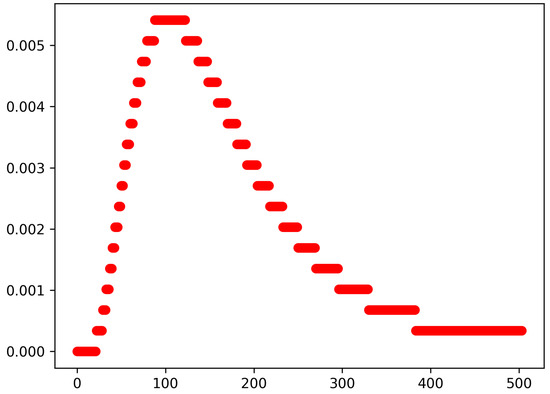
Figure 1.
The empirical density function of the sequence .
4.3. The Effect of Network Size on Approximation Accuracy
In this test, we experimentally observe the effect of network size on approximation accuracy. For a sequence of networks with increasing network size, we compare the degree distributions returned by the approximation method (Algorithm 4) to the exact degree distributions computed by Algorithm 2. We use the total variation distance for comparison. When the approximator uses the Poisson or the binomial distributions, we can directly use the total variation distance; however, when the Gaussian distribution is used for approximation, we use the following discretization to obtain a discrete probability distribution: if X is a continuous random variable with cdf, then its discretized version has a pdf:
To create the test IRG parametrizations, we used the biased static edge voting model using lognormal and range parametrization methods. For both cases, the network sizes are 50, 100, 300, 500, 1000, 1500, 2000, 2500, and 3000.
We denote the biased static edge voting model with parametrization and by , and the IRG generated from using (66) by . It is clear that in , for all different nodes a and b, . Similarly, we denote the static edge voting model with parametrization by , and the IRG generated from using (66) by . The values of and for the parametrization for each n can be found in Table 1. Because of the construction, has a block structure. It contains clusters, and within a cluster, the nodes have the same degree distribution. In Table 1, we collected basic statistics about the clusters for the used parametrizations.

Table 1.
Node cluster size statistics of different parametrizations. Size: number of nodes. Parametrization: Parameters of the lognormal sequence parametrization methods. Nr of clusters: number of node clusters. Mean: mean size of node clusters. Sd: standard deviation of node cluster size. Min; max: minimum and maximum node cluster size.
Let us denote the exact degree distribution of computed with Algorithm 2 by , where T can be R or . Similarly, we denote the approximated degree distribution of computed with Algorithm 4 by , where T can be R or and G stands for the used approximation distribution: P (Poisson), B (binomial), or G (Gaussian). For example, we denote the approximated degree distribution of using the Poisson distribution by . We calculated the total variation distance between the approximated and the exact degree distribution:
The calculated values are collected in Table 2 and Table 3. We also plotted the total variation distances in the function of the network size in Figure 2 and Figure 3. We can observe that in the case of the parametrization, the approximation error monotonically decreases with the network size, and we achieve the best approximation using the Gaussian approximation. At the parametrization, we can observe an initial fluctuation in the approximation error, and after this, there is a monotone decreasing trend in the approximation error in function of the network size. In this case, we obtain the smallest approximation error when we use the binomial distribution.
Table 2.
Total variational distance between the approximated and the exact degree distributions when the IRG is created using parametrization.
Table 3.
Total variational distance between the approximated and the exact degree distributions when the IRG is created using parametrization.
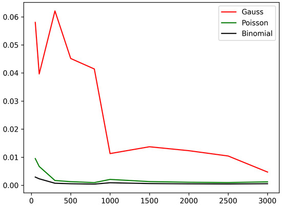
Figure 2.
Total variational distance between the approximated and the exact degree distribution in the function of network size when the IRGs are generated by parametrization of the biased static edge voting model.
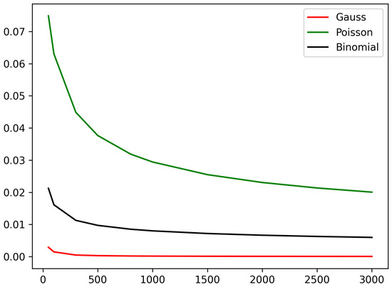
Figure 3.
Total variational distance between the approximated and the exact degree distribution in the function of network size when the IRGs are generated by parametrization of the biased static edge voting model.
4.4. The Effect of Cluster Size on Approximation Accuracy
In this experiment, we test how the accuracy of the approximation method depends on the cluster size. denotes the IRG model generated from the biased edge voting model with parametrization using (66). This IRG is “very inhomogeneous” in the sense that all edge probabilities are different; therefore, the degree distribution of each node is different. We compute the exact degree distribution of using Algorithm 2 and denote the result by . We plotted in Figure 4.
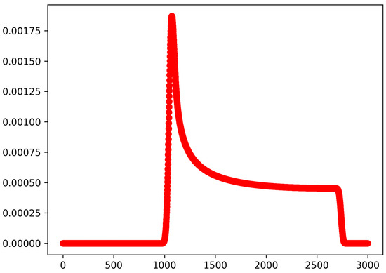
Figure 4.
The exact degree distribution of the IRG generated by the biased static edge voting model with parametrization.
We denote the number of nodes by n ( in the current setting) and identify the nodes by their parameter in the static edge voting model used to generate the . This means that for any node, the parameter of the node in the generator biased edge voting model was a. Let us fix a cluster size and suppose that n is divisible by S. We define a partition of as:
The degree distributions of all nodes within a cluster of partition are different. We tested the approximation method described in Section 3.3, where the node clusters are given by , and the S cluster size is in = {1500, 1000, 750, 600, 500, 300, 200, 100, 75, 60, 50, 30, 20, 10, 5, and 1}. For example, if the S cluster size is 1000, then we have 3 node clusters: . We computed the approximated degree distribution of using Algorithm 4 and denoted the result distributions by , where S denotes the cluster size and D represents the type of distribution used in the approximation, which can be P (Poisson), B (binomial), or G (Gaussian). For all S cluster sizes from , we calculated the total variation distance between the exact degree distribution (plotted in Figure 4) and the approximated degree distributions:
The results are collected in Table 4 and plotted in Figure 5. We can observe that the approximation error decreases as the cluster shrinks (or the number of clusters increases). If the cluster size is huge, then the Poisson approximation gives the smallest approximation error, while if the clusters are small, the Gaussian approximation gives the best results, although in the case of small clusters, the difference between the approximators is small.
Table 4.
Total variational distance between the approximated and the exact degree distribution when the IRG is created using parametrization and the clusters are given by .
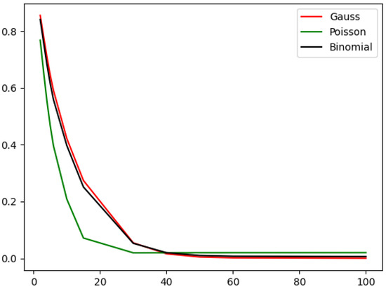
Figure 5.
Total variational distance between the approximated and the exact degree distribution in the function of cluster numbers, where the IRG is generated using the parametrization and the clusters are given by .
5. Discussion
Inhomogeneous random graph is a random graph model where the links of the graph are drawn independently and the link probabilities can be different. It can be seen as the generalization of the Erdős–Rényi random graph [15], where the edges are drawn independently, but the probability that any different two nodes are linked is a fixed p value. The degree distribution of a deterministic or random graph with n nodes is defined as the probability that the degree of a uniformly chosen node equals to k for all . The degree distribution has a central role in network science, not only because it is needed to compute several other network properties [1], but also because the shape of the degree distribution mostly determines the outcome of many important network processes, such as the spread of viruses [5], diffusion of innovations [6,7], or attacks against critical infrastructure [2,3,4]. The degree distribution of many real-world networks have fat tails; therefore, the ER random graph model is not suitable to model real world networks, because its degree distribution is binomial [15]. Therefore, many alternative random graph models have been proposed to be able to model real world networks, such as the stochastic block model [8], generalized random graphs [12], Chung–Lu random graphs [16], the Norros–Reittu model [17], and the static edge voting model [14] (Section 4.2), which we used to generate the appropriate IRG parametrisations to test our algorithms in Section 4. Using different parametrizations of the IRG model, one can achieve random network models with very different degree distributions. IRG is interesting not only as the generalization of the ER random graph but also as a tool to analyse other random graph models, such as the stochastic block model, generalized random graphs, or the static edge voting model.
In this paper, we focused on the calculation of the degree distribution of the IRG model. In Section 3.2, we discussed an algorithm to compute the exact degree distribution utilizing the DFT-CF method [19] developed by Yili Hong. The proposed algorithm (Algorithm 2) is highly parallelizable since the sub-step given in Algorithm 3 can be called independently. Furthermore, if the IRG model has a block structure, Algorithm 2 can take advantage of it. In Section 3.3, we presented a method to approximate the degree distribution of the IRG model. There are several reasons why one would apply approximation even if an exact computational method is available. One reason is that approximation is computationally cheaper than the exact method. A second reason is that the approximation method may also be used in the case when the IRG is not fully defined. At the beginning of Section 3.3, we discussed the general scheme of the proposed approximation method, which is presented in Algorithm 4. The idea of the approximation method is simple: we group the nodes of the network according to their statistical behaviour. For each node group, we approximate the common behaviour of the nodes within the group, and finally, we aggregate these group approximations. As a result, we obtain a mixture model, which we use as an approximation of the exact degree distribution. Similarly to the exact algorithm, it can be implemented effectively in a multi-thread environment. In Algorithm 4, we did not specify how to approximate the common behaviour of a node group, because it can be done in many ways, but in the subsequent subsections, we analysed three possible ways: using the Poisson distribution (Section 3.3.1), the binomial distribution (Section 3.3.2), and the Gaussian distribution (Section 3.3.3). Furthermore, we derived an upper bound for the approximation error for all three cases: Equation (48) for the Poisson and the binomial approximations, and Equation (60) for the Gaussian approximation.
Determining which distribution to use for optimal results is a natural question. Unfortunately, we do not have a clear answer to this. During the numerical experiments in Section 4, we found that the structure of the IRG and the granularity of the clustering influences which distribution will lead to the most accurate approximation. In Section 4.3, we tested the approximation method on IRG models having a block structure (see Figure 2 and Table 2), where within each block, the nodes obey the same degree distribution. In this case, we could observe that using the binomial distribution gave the most accurate results. However, in the case where the degree distribution of each node was different and we did not apply grouping, using the Gaussian distribution gave the best results (see Figure 3 and Table 3). In Section 4.4, we tested the effect of the clustering granularity on the approximation precision. We fixed an IRG model where the degree distribution of each node is different and applied the approximation with clustering, where the cluster size was different for each test case. We found that for larger cluster sizes, the usage of the Poisson distribution gave the most accurate estimate, and for smaller cluster sizes, the Gauss distribution gave the best results (see Figure 5 and Table 4).
The approximation method can be extended or improved in several ways. In this study, we analysed the usage of Poisson, binomial and Gaussian distributions. However, there are other distributions that we could use in a similar way. One obvious possibility is using the PB distribution itself. Another candidate for this is the translated Poisson distribution [20,33] or the Pólya approximation of the PB distribution [34]. Another direction can be the optimal selection of the group approximation method. We have seen in Section 4.3 and Section 4.4 and in the previous paragraph that the structure of the IRG and the granularity of the clustering influences which distribution will lead to the most accurate approximation. It is an open question if we can implement a selection method to find the optimal approximator distribution.
Author Contributions
Conceptualization, R.P.; methodology, R.P.; software, R.P.; validation, R.P.; investigation, R.P.; writing—original draft preparation, R.P.; writing—review and editing, L.K. and R.P.; supervision, L.K.; project administration, L.K.; funding acquisition, L.K. All authors have read and agreed to the published version of the manuscript.
Funding
Project no. 2019-1.3.1-KK-2019-00007 has been implemented with the support provided from the National Research, Development and Innovation Fund of Hungary, financed under the 2019-1.3.1-KK funding scheme. This project has been supported by the Hungarian National Research, Development and Innovation Fund of Hungary, financed under the TKP2021-NKTA-36 funding scheme.
Data Availability Statement
The source code of the numerical experiments is available at https://github.com/rpethes/IRG (accessed on 11 February 2023).
Conflicts of Interest
The authors declare no conflict of interest.
Appendix A
We calculate if . First, derive the antiderivative of . From linearity of integral:
Let’s continue with the indefinite integral . Applying the substitution :
The antiderivative of is [35], therefore:
Therefore:
Since and :
References
- Barabási, A.-L. Network Science; Cambridge University Press: Cambridge, UK, 2016. [Google Scholar]
- Albert, R.; Jeong, H.; Barabási, A.-L. Attack and error tolerance of complex networks. Nature 2000, 406, 378. [Google Scholar] [CrossRef] [PubMed]
- Cohen, R.; Erez, K.; ben-Avraham, D.; Havlin, S. Resilience of the Internet to random breakdowns. Phys. Rev. Lett. 2000, 85, 4626. [Google Scholar] [CrossRef] [PubMed]
- Cohen, R.; Erez, K.; ben-Avraham, D.; Havlin, S. Breakdown of the Internet under intentional attack. Phys. Rev. Lett. 2001, 86, 3682. [Google Scholar] [CrossRef] [PubMed]
- Pastor-Satorras, R.; Vespignani, A. Epidemic spreading in scalefree networks. Phys. Rev. Lett. 2001, 86, 3200–3203. [Google Scholar] [CrossRef] [PubMed]
- Valente, T.W. Network Models of the Diffusion of Innovations; Hampton Press: Cresskill, NJ, USA, 1995. [Google Scholar]
- Rogers, E.M. Diffusion of Innovations; Simon and Schuster: New York, NY, USA, 2010. [Google Scholar]
- Holl, P.W.; Laskey, K.B.; Leinhardt, S. Stochastic blockmodels: First steps. Soc. Netw. 1983, 5, 109–137. [Google Scholar]
- Karrer, B.; Newman, M.E.J. Stochastic blockmodels and community structure in networks. J. Phys. Rev. E 2011, 83, 016107. [Google Scholar] [CrossRef]
- Barabási, A.; Oltvai, Z.N. Network biology: Understanding the cell’s functional organization. Nat. Rev. Genet. 2004, 5, 101–113. [Google Scholar] [CrossRef]
- Buhl, J.; Gautrais, J.; Reeves, N.; Solé, R.V.; Valverde, S.; Kuntz, P.; Theraulaz, G. Topological patterns in street networks of self-organized urban settlements. Eur. Phys. J.-Condens. Matter Complex Syst. 2006, 49, 513–522. [Google Scholar] [CrossRef]
- Tom, B.; Deijfen, M.; Martin-Löf, A. Generating simple random graphs with prescribed degree distribution. J. Stat. Phys. 2006, 124.6, 1377–1397. [Google Scholar]
- Van Der Hofstad, R. Random Graphs and Complex Networks; Cambridge University Press: Cambridge, UK, 2016. [Google Scholar]
- Róbert, P.; Kovács, L. Voting to the link: A static network formation model. Acta Polytech. Hung. 2020, 17, 207–228. [Google Scholar]
- Erdős, Paul and Alfréd Rényi On the evolution of random graphs. Publ. Math. Inst. Hung. Acad. Sci. 1960, 5, 17–60.
- Chung, F.; Chung, F.R.; Graham, F.C.; Lu, L. Complex Graphs and Networks; No. 107; American Mathematical Soc.: Providence, RI, USA, 2006. [Google Scholar]
- Ilkka, N.; Reittu, H. On a conditionally Poissonian graph process. Adv. Appl. Probab. 2006, 38, 59–75. [Google Scholar]
- Barabási, A.; Albert, R. Emergence of scaling in random networks. Science 1999, 286, 509–512. [Google Scholar] [CrossRef] [PubMed]
- Hong, Y. On computing the distribution function for the Poisson binomial distribution. Comput. Stat. Data Anal. 2013, 59, 41–51. [Google Scholar] [CrossRef]
- Tang, W.; Tang, F. The Poisson binomial distribution—Old & New. Stat. Sci. 2022, 1, 1–12. [Google Scholar]
- Cooley, J.W.; Tukey, J.W. An algorithm for the machine calculation of complex Fourier series. Math. Comput. 1965, 19, 297–301. [Google Scholar] [CrossRef]
- Saks, S. Theory of the Integral; Warszawa–Lwów: G.E. Stechert & Co.: New York, NY, USA, 1937. [Google Scholar]
- Total Variation. Available online: https://handwiki.org/wiki/Total_variation (accessed on 21 January 2023).
- Rudin, W. Functional Analysis, 2nd ed.; McGraw-Hill: New York, NY, USA, 1991. [Google Scholar]
- Barbour, A.D.; Hall, P. On the rate of Poisson convergence. In Mathematical Proceedings of the Cambridge Philosophical Society; Cambridge University Press: Cambridge, UK, 1984; Volume 95. [Google Scholar]
- Janson, S. Coupling and Poisson approximation. Acta Appl. Math. 1994, 34, 7–15. [Google Scholar] [CrossRef]
- Adell, J.A.; Jodrá, P. Exact Kolmogorov and total variation distances between some familiar discrete distributions. J. Inequalities Appl. 2006, 2006, 1–8. [Google Scholar] [CrossRef]
- Ehm, W. Binomial approximation to the Poisson binomial distribution. Stat. Probab. Lett. 1991, 11, 7–16. [Google Scholar] [CrossRef]
- Choi, K.P.; Xia, A. Approximating the number of successes in independent trials: Binomial versus Poisson. Ann. Appl. Probab. 2002, 12, 1139–1148. [Google Scholar] [CrossRef]
- Billingsley, P. Probability and Measure; John Wiley & Sons: Hoboken, NJ, USA, 2008. [Google Scholar]
- Petrov, V.V. Sums of Independent Random Variables; De Gruyter: Berlin, Germany, 2022. [Google Scholar]
- Spivak, M. Calculus, 4th ed.; Cambridge University Press: Cambridge, UK, 2008. [Google Scholar]
- Röllin, A. Translated Poisson approximation using exchangeable pair couplings. Ann. Appl. Probab. 2007, 17, 1596–1614. [Google Scholar] [CrossRef]
- Skipper, M. A Pólya approximation to the Poisson-binomial law. J. Appl. Probab. 2012, 49, 745–757. [Google Scholar] [CrossRef]
- Inverse Trigonometric Functions. Available online: https://en.wikipedia.org/wiki/Inverse_trigonometric_functions (accessed on 21 January 2023).


Disclaimer/Publisher’s Note: The statements, opinions and data contained in all publications are solely those of the individual author(s) and contributor(s) and not of MDPI and/or the editor(s). MDPI and/or the editor(s) disclaim responsibility for any injury to people or property resulting from any ideas, methods, instructions or products referred to in the content. |
© 2023 by the authors. Licensee MDPI, Basel, Switzerland. This article is an open access article distributed under the terms and conditions of the Creative Commons Attribution (CC BY) license (https://creativecommons.org/licenses/by/4.0/).