Abstract
The analysis of global epidemics, such as SARS, MERS, and COVID-19, suggests a hierarchical structure of the epidemic process. The pandemic wave starts locally and accelerates through human-to-human interactions, eventually spreading globally after achieving an efficient and sustained transmission. In this paper, we propose a hierarchical model for the virus spread that divides the spreading process into three levels: a city, a region, and a country. We define the virus spread at each level using a modified susceptible–exposed–infected–recovery–dead (SEIRD) model, which assumes migration between levels. Our proposed controlled hierarchical epidemic model incorporates quarantine and vaccination as complementary optimal control strategies. We analyze the balance between the cost of the active virus spread and the implementation of appropriate quarantine measures. Furthermore, we differentiate the levels of the hierarchy by their contribution to the cost of controlling the epidemic. Finally, we present a series of numerical experiments to support the theoretical results obtained.
MSC:
49K15
1. Introduction
Global epidemics provide a serious medical challenge worldwide. Millions of mortality cases each year are estimated to be directly related to infectious diseases [1]. Attempts to suppress the spread of infections are usually divided into pharmaceutical and non-pharmaceutical interventions: for example, several different vaccines against the novel coronavirus were developed quickly and were available within months of the onset of the epidemic; on the other hand, measures were taken to reduce the interregional and urban mobility of citizens, and the so-called lockdowns [2]. The relationship between these measures and the trade-off in choosing the appropriate response to an epidemic is the subject of much research on epidemic prevention [3,4,5].
The main tool for studying the effectiveness of various intervention policies is the mathematical modelling of the spreading processes [6,7,8,9]. Both types of interventions are reflected in the work of researchers—both pharmaceutical [10,11] and non-pharmaceutical [3,12,13,14] interventions. In our model, we combine these types of interventions, introducing the treatment as a controlled parameter and vaccination as an exogenous one, while allowing the population to enter a state of self-isolation or quarantine. Importantly, we divide the population into several related levels, the size and configuration of the links between which allow us to interpret them as hierarchical levels.
The idea of differentiating populations in epidemic models according to different characteristics is not novel. In the COVID-19 period, many predictive models were based on the classical SEIR, but were a tuple of such models, each relating to a different age group (see, for example [15,16,17,18,19]. On the other hand, so-called spatial models of the epidemic spread, which also distinguish populations on a territorial basis, became widespread: this gave rise first to the metapopulation or multi-group/multi-cluster epidemic models [20,21,22], and later to network models (an overview of such models is provided, for example, in [23]).
In the current research, we were motivated by the unprecedented outbreak of COVID-19 that began in one location in China and spread throughout the world [24]. We assumed the epidemic process could be divided into several hierarchical levels or clusters: a city, a region, and a country. Depending on the size of the population in each level/cluster, the pathogen’s spread rate will differ. These assumptions lead to a hierarchical model with three levels and the possibility of migration between levels. Epidemics are assumed to originate from the first cluster, which is the smallest, and spread to the second and third clusters based on infection and migration rates. In this paper, we formulate the hierarchical epidemic model with controls, considering the quarantine and vaccination as countermeasures against the spread of the virus. The model assumes that quarantine measures can only be applied at the first level of the system, while vaccination and treatment can be applied at any level. We focus on the first cluster in the proposed model, as it has the potential to halt the spread of infection at the local level and prevent further transmission. Our aim is to investigate the effectiveness of a combination of different control strategies and compare their effectiveness.
In our previous work [25], we investigated the unidirectional spread of infection: from the initial level to the subsequent ones. Such dynamics were interpreted as the migration of individuals through land/air transport from the local level to the next. However, there is also an inverse relationship: even under the threat of infection, individuals migrate between levels and, among other things, can return to the source of infection due to compelling individual reasons: be it economic reasons, such as a place of study or work, or personal reasons, for example, the permanent residence of relatives and friends. Therefore, in this model, we modified the mechanism for the transition of individuals between levels. At the same time, the infection continues to initialize on the first layer and spreads in the direct path—from the first level, through the second and to the third, and in the opposite direction—from the third through the second back to the first. A difference from the previous work is the addition of a dead subgroup and analysis of the basic reproductive number for our model. We also added the vaccination process, which is one of the effective methods of preventing the spread of the epidemic.
We present the optimal control problem for the hierarchical epidemic model with a intra-level migration and analyze the structure of the optimal protective measures. The analysis of the model includes the construction of the basic reproduction number to estimate the impact of the different parameters on the propagation of the pathogen in the different clusters. A series of numerical experiments are proposed to support the received theoretical results.
This paper is organized as follows: Section 2 introduces the initial model, Section 3 analyzes the system and the basic reproduction number, Section 4 formulates the optimal control problem and presents the structure of the optimal control strategies, Section 5 provides numerical simulations to validate the theoretical results, and Section 6 summarizes the main findings and concludes the paper.
2. Deterministic Epidemic Model
In contrast to classical SIRS models, which divide populations into three groups, this section presents a modified SQEIRD model (susceptible–quarantined–exposed–infected–recovered–dead) with three levels. The model considers one virus circulating in a population of size N and enables us to capture epidemic processes occurring on different levels. These levels can be defined as individual regions, villages, cities within a country, or different countries.
We assume that if an epidemic is initiated in a small village (the first cluster), it can extend to a city, region, or country (the second and third clusters). We formalize this epidemic situation in a mathematical model. Virus propagation starts at the first level of the hierarchy and continues on the i-th levels, , based on migration rates. The spreading process is modeled using a susceptible–quarantined–exposed–infected–recovered–dead (SQEIRD) model at the first level hierarchy. This model divides the population into six subgroups: susceptible (S), quarantined (Q), exposed (E), infected (I), recovered (R), and dead (D). The susceptible agents are at risk of contracting the virus, and the recovered agents are immune. The quarantined agents are isolated and cannot come into contact with potentially infected agents, making them immune to infection. In this model, vaccination is used in the susceptible groups as a protection measure. WHO reports have demonstrated that vaccination is the most effective way to protect the population from infectious diseases. There is a risk of breaking quarantine rules and coming into contact with an exposed or infected agent, which increases the probability of infection.
The pathogen comes from infected and exposed subgroups into contact with susceptible and quarantine individuals that they have never before encountered. Members of the recovered subgroup receive the immunity as a result of a disease or vaccination. We assume that a subset of the exposed group in the population can transmit the virus without developing symptoms. Unlike the first cluster, the second and third clusters consist of the following subgroups: susceptible , exposed , infected , recovered , and dead . The susceptible group in all clusters can transition to the exposed group at a rate of , . Exposed agents develop symptoms and become infected at the rate of , . The self-recovery rates are the same in all clusters, and are defined as , . The parameter indicates the rate at which susceptible agents choose isolation and become quarantined. With probability p, residents from the Quarantine group can contact an agent from the Exposed group and become exposed with a rate of . Vaccination is represented by a parameter , which allows susceptible agents to become immune to the virus and belong to the recovered subgroup. The death rate at level i is denoted by . Additionally, we assume that migration occurs between clusters, and that migration rates are , , and . The transition scheme is illustrated in Figure 1.
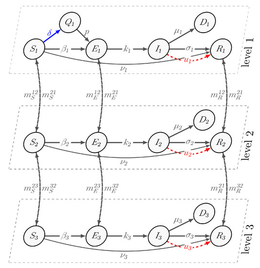
Figure 1.
The scheme of transition between groups S, Q, E, I, R, D, and hierarchical levels.
We describe the epidemic process as a set of nonlinear differential equations, where denotes the population size at level i at time t. Specifically, represents the number of susceptible individuals, represents the number of quarantined individuals, represents the number of exposed individuals, represents the number of infected individuals, represents the number of recovered individuals, and represents the number of dead individuals. The following conditions must be satisfied: , for , and .
Based on the above definitions, the variables , , , , , and indicate the proportions of susceptible, quarantined, exposed, infected, recovered, and dead individuals at time , where
At the start of the epidemic (), the majority of individuals are in the susceptible state, and only a small fraction are infected. The initial states for all levels are as follows:
- , , , ;
- , ;
- .
The set of nonlinear differential equations describes the spread of the virus in each cluster/level of the population. On the first level:
On the second level:
On the third level:
3. Basic Reproduction Number
This section employs the next generation method (NGM) [26,27] to estimate the basic reproduction number in the model (1)–(3), which represents the average number of cases of an infectious disease that arise via transmission from a single infected individual and approximates the asymptotic behavior of an epidemic process. The value of is crucial in evaluating the infection propagation in the entire population, as the number of infected individuals will asymptotically decrease if , and increase otherwise.
The NGM method involves transforming the original system into , where the matrices F and V are given by and , respectively. Here, i refers to the indices of all infected state variables in the initial system of differential equations.
In the model (1)–(3), all states can be divided into two groups: infected and non-infected states. Specifically, the infected states are , and therefore, the matrices F and V have a size of , according to NGM. These matrices are presented below.
Disease-free equilibrium:
According to the NGM, the maximum value of the absolute eigenvalues of is equal to the reproduction number . Numerically estimating various parameter combinations, we found that migration only has a significant impact when or differs across levels . The diagrams below depict how varies with different parameters. In the following numerical experiments, we used the following parameter values, unless otherwise specified: , , , , .
As shown in the left diagram of Figure 2, the reproduction number, , varies linearly with the infection rate, , and decreases as the control increases. On the other hand, the right diagram of Figure 2 depicts as a function of the migration rate, , and control, which takes the shape of an almost constant hyperbola when the migration rate exceeds 0.5. This diagram also demonstrates that the reproduction number decreases as the control increases, and can fall below 1 even without the control if the migration rate exceeds 0.5.
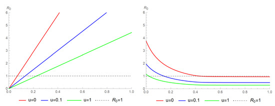
Figure 2.
The diagram on the left illustrates how the reproduction number depends on the infection rate, , for different constant controls, . Meanwhile, the diagram on the right demonstrates how the reproduction number varies with the migration rate, , for different constant controls, u.
4. Optimal Control Problem
The focus of the present study is to formulate an optimal control problem aimed at minimizing the damage caused by virus outbreaks and enhancing the protection of the population. The model employed in this study assumes that quarantine and treatment measures can shield the population from viral transmission. At each level of the hierarchical structure, treatment is applied as a control strategy , , for infected nodes (), if the epidemic extends across all levels due to migration rates. To estimate the infection costs, the method proposed in [10,11,12] is adopted, which includes direct losses suffered by an infected person, such as treatment expenses, loss of productivity, and incapacity. The treatment costs, which indicate the value spent by the government to facilitate the health care system’s ability to treat infected individuals and enhance the probability of their recovery, are considered as external costs.
Cost functions: The costs associated with infections and treatments are represented by functions and , respectively, at any given time t. These functions must satisfy certain conditions. The functions are non-decreasing, twice-differentiable, and convex, with and for , where . Similarly, the functions are twice-differentiable and increasing in , with and for when .
The functional for the aggregated system costs on the time interval is defined as follows:
where
The goal of the optimal control problem is to minimize the costs given by the functional J:
By applying Pontryagin’s maximum principle [28,29], we can construct the Hamiltonian and adjoint functions. The generalized Hamiltonian of the system is given as follows: . Hamiltonian of the first level:
Hamiltonian of the second level:
Hamiltonian of the third level:
The adjoint functions of the first level are defined as follows: , , , , and .
The transversality conditions are given by:
Analogously, adjoint functions , , , and of the second level are:
with the transversality conditions given by
Adjoint functions , , , and of the third level:
with the transversality conditions given by
The existence of continuous and piece-wise continuously differentiable co-state functions
which satisfy (9)–(14) at every time , together with continuous functions , , and , is guaranteed by Pontryagin’s maximum principle:
Following the Pontryagin’s maximum principle [11,28,29,30,31], we should analyze the behaviour of the derivative . We obtain that
We denote the last terms in (16) as switching functions , :
Proposition 1.
Assuming that functions are concave, the optimal control structure is expressed as follows for :
Proposition 2.
If are strictly convex functions, the optimal control structure is as follows for any
where .
To prove these propositions, we can rewrite the Hamiltonian in terms of the function . After that, we obtain:
The optimization problem can be decomposed into three subproblems, where we consider the optimal controls , and separately. This can be achieved by solving:
For any admissible control , and for all according to (20), we have:
As is an admissible control, we obtain:
To determine the optimal control structure using Pontryagin’s maximum principle, we consider the following derivatives:
Given that are increasing functions and , we can maximize the Hamiltonian by ensuring that for , as stated in the proposition. Using Equation (17) and the fact that for all , we can rewrite this condition as for .
To complete the proof of the proposition, we need to establish Lemma 1:
Lemma 1.
For all , we have , .
The proof of Lemma 1 consists of two parts. First, we consider the case when and show that the derivatives of the functions , , are non-positive. Second, we prove by contradiction the negativity of these functions on the whole interval . The complete proofs of Lemma 1 follow the same technique as that in [11,30].
Note that since are increasing functions, the Hamiltonian is convex in , if are also concave, i.e., , according to Equations (6)–(8). As a result, there are two different options for that maximize the Hamiltonian, where .
If or , then the optimal control is (see Figure 3(left)). Otherwise, the optimal control is (see Figure 3(right)).
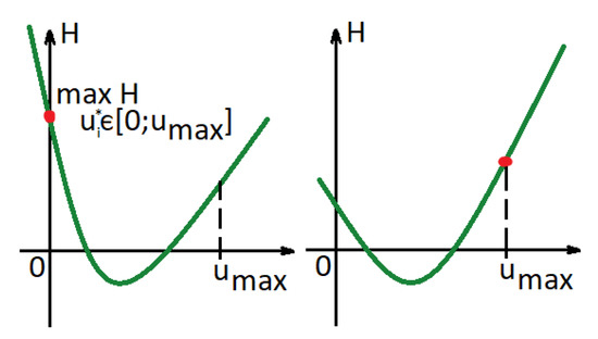
Figure 3.
Hamiltonian function in a case in which functions are concave.
4.1. Functions Are Concave
Assuming is a concave function with , it follows from (6)–(8) that the Hamiltonian is a convex function of for . There exist two possible values of that maximize the Hamiltonian, where .
For the optimal control parameters are defined as follows:
4.2. Functions Are Strictly Convex
Assuming is a strictly convex function (), the Hamiltonian is a concave function. We consider the derivative:
where , , and . There exist three different types of points at which the Hamiltonian reaches its maximum (Figure 4). To find them, we need to consider the derivatives of the Hamiltonian at and . If the derivatives (26) at are non-increasing (), then the value of the control that maximizes the Hamiltonian is less than 0, and according to our restrictions (), the optimal control will be equal to 0 (Figure 4 (left)). If the derivatives at are increasing (), this implies that the value of the control that maximizes the Hamiltonian is greater than . Hence, the optimal control will be 1 (Figure 4 (right)). Otherwise, we can find the value of (see Figure 4 (middle)):
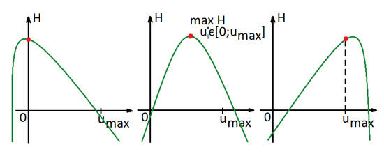
Figure 4.
Hamiltonian function in a case in which functions are convex.
5. Numerical Simulation
In this section, we conduct a series of numerical experiments to validate our findings. We consider a country with a population of 10,000,000, where the first level has 1,500,000 residents, the second level has 3,000,000 residents, and the third level has 5,500,000 residents. The time interval is one year ( days).
We start with the following initial distribution among susceptible, exposed, and infected groups: , , and , which correspond to 10,000 exposed and 1000 infected residents at . The transmission rate is , and the self-recovery rate is , which takes approximately 21 days for a resident to recover from the virus without any treatment [32]. The incubation period is for . We assume that symptoms appear after about 6 days, and exposed residents become infected. The cost functions for the infected group are , and the treatment cost functions are defined as for . In this model, we assume that the maximum value of the control is . More details about the parameters and initial data used in the experiments can be found in Table 1.

Table 1.
Parameters used for simulations in experiments.
Experiment 1. In the current experiment, we present the SQEIRD model under the assumption that the quarantine and vaccination are not possible for susceptible individuals (, , and ). Using the specially developed procedure and taking into consideration the cluster structure of the population, we obtain the result that the epidemic starts and reaches its maximum faster on the first level than on levels 2 and 3 in the uncontrolled case. At the second and the third clusters, the epidemic starts with delays. Figure 5 and Figure 6 demonstrate this fact.
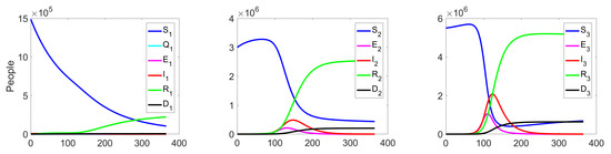
Figure 5.
Experiment 1. Spread of the virus in three different clusters in an uncontrolled case.
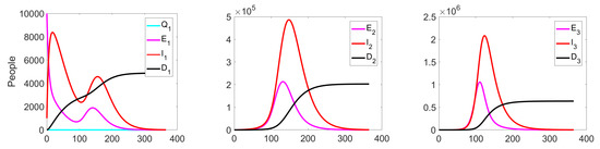
Figure 6.
Experiment 1. Number of Exposed, Infected, and Dead in uncontrolled case.
The behaviour of the system in the controlled case is shown in Figure 7. We can notice a significant decrease in the number of the infected at all levels, which leads to a reduction in costs (see Figure 8c).
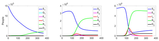
Figure 7.
Experiment 1. Spread of the virus in three different clusters in a controlled case.
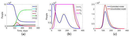
Figure 8.
Experiment 1. (a) Sum of the fractions of all levels in controlled case; (b) the structure of the optimal treatment policies , ; (c) aggregation costs in uncontrolled and controlled cases.
Figure 9 shows the change in the fractions of the exposed, infected, and dead population at all three levels. Since we do not apply any quarantine measures, the fraction is equal to zero on all considered intervals .
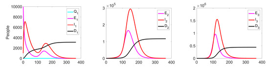
Figure 9.
Experiment 1. Number of exposed, infected, and dead in controlled case.
Figure 8 summarize the changes in all fractions of the population (Figure 8a), the optimal treatment policies structure (Figure 8b), and the aggregate system costs. In the uncontrolled case, the costs are equal to monetary units (m.u.), while in the controlled case, they are m.u. (Figure 8c).
Experiment 2. In the current experiment, we consider the SQEIRD model with quarantine and vaccination. We assume that the government has an access to a vaccine that forms an acquired immunity to the virus and also has imposed quarantine measures.
This experiment shows the effects of vaccination and quarantine measures on the development of an epidemic situation. The behavior of the system in the controlled case is shown in Figure 10.
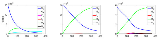
Figure 10.
Experiment 2. Spread of the virus in three different clusters in the controlled case.
Figure 11 shows the change in the fractions of the quarantined, exposed, infected, and dead population at all three levels. According to the quarantine measures, the citizens should stay at home, but there is a small fraction of residents that do not comply with these measures, which leads to their infection.
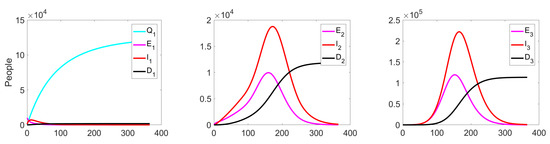
Figure 11.
Experiment 2. Number of Exposed, Infected, and Dead in controlled case.
Figure 12a shows the aggregate changes in all fractions of the population, while Figure 12b represents the structure of the optimal treatment policies , . The controlled case results in a significantly lower aggregated system cost of m.u. compared to the uncontrolled case’s cost of m.u. (Figure 12c).
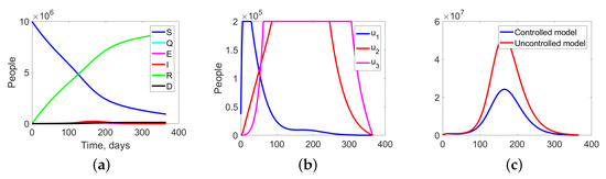
Figure 12.
Experiment 2. (a) Sum of the fractions of all levels in controlled case; (b) the structure of the optimal treatment policies , ; (c) aggregation costs in uncontrolled and controlled cases.
The implementation of quarantine measures and vaccination in the optimal control strategy leads to a reduction in the overall epidemic spread, with a maximum number of infected individuals of on the third level, which is much lower than the peak observed in Experiment 1. Additionally, the peak of infected residents on the third level occurs later, on the 168th day, as opposed to Experiment 1, where it occurred on the 126th day. These results suggest that optimal controllers can effectively conserve the health system’s resources, including medical staff and equipment, and prevent its collapse.
Experiment 3. In this experiment, we examine the impact of agent responsibility on the system’s behavior.
First, we consider a scenario in which all individuals are responsible for their actions (Experiment 3a). It is assumed that taking responsibility for their actions has a positive effect on the overall epidemic spread and minimizes the overall costs. Residents voluntarily remain in quarantine throughout the time interval T = [0;365]. The transition from the susceptible subgroup to quarantine (voluntary self-isolation) occurs at a rate of , which is higher than in Experiment 2 (). However, in contrast to the previous case, the transition rate from quarantine to the exposed subgroup is equal to , which is lower than in the previous experiment. All other system parameters remain the same. In this section of the experiment, we investigate the impact of agent responsibility on the behavior of the system. In Experiment 3a, we assume that all individuals are responsible for their actions, and residents voluntarily remain in quarantine until the end of the interval T = 365. The transition rate from the susceptible subgroup to the quarantine subgroup (voluntary self-isolation) is , which is higher than in Experiment 2 (). However, unlike the previous case, the transition rate from the quarantine to exposed is , which is lower than in Experiment 2. The other parameters of the system remain the same.
Our results demonstrate that the peak number of infected agents is lower in Experiment 3a () than in the case where residents leave quarantine independently without the government’s consent (). The total system costs in the uncontrolled case are m.u., while in the controlled case, they are m.u. Comparing these costs with those of the previous experiment confirms the hypothesis that the general responsibility of residents in the population leads to lower overall epidemic costs.
In Experiment 3b, we assume that all individuals in the population are irresponsible and prefer to violate the quarantine isolation rules. Under this assumption, the transition rate from susceptible to quarantined subgroups is , which is lower than in Experiments 2 and 3a. At the same time, quarantined individuals become exposed at a higher rate of compared to the case of responsible residents. All other parameters remain the same. The peak number of infected agents is equal to . It can be noted that the irresponsibility of residents leads to the rapid spread of the virus and a larger number of infected individuals even in the controlled case. Aggregate system costs in the uncontrolled case are equal to m.u., compared to m.u. in the controlled case. Comparing the costs with the previous experiment, the hypothesis of the general responsibility of residents in the population is also confirmed. The irresponsible residents increase the aggregated cost of the epidemic.
Experiment 4. In this experiment, we conduct a series of experiments, in each of which, we switch the control on and off at different levels. After that, we compare the resulting costs at each individual level. All parameters are taken the same as in Experiment 2. In this case, we run a series of experiments, in which we turn the control on and off at different levels. We then compare the resulting costs at each level. Costs at level i are , . We decided to look at five different cases:
- Switching on optimal control at all three levels;
- Switching on optimal control at levels 1 and 2;
- Switching on optimal control at level 1 only;
- Switching on optimal control at levels 2 and 3;
- Without any control (uncontrolled case).
We decided to investigate the effect of control at different levels on the total cost of the epidemic. Table 2 shows the relative costs at each level and the total costs J. We took the uncontrolled case as the baseline and compared all the other costs to it, by dividing our costs by the costs in the uncontrolled case.
Table 2.
Costs on each level relative to the costs in uncontrolled case.
As a result, two theses can be identified. The first thesis is the more obvious one. Switching on the optimal control at a level results in a reduction in cost at that level compared to the cost in the case without the control. The second thesis is a little less obvious. If we take into account the total costs in each of the experiments, the following trend can be observed. Switching on the optimal control on the third level leads to a reduction in overall costs. This effect is due to the fact that the migration rate is greater from level 1 to level 2 and from level 2 to level 3 than in the opposite direction. Many agents migrate to level 3 to avoid the epidemic, but at the same time, asymptomatic agents in the exposed subgroup migrate and bring the epidemic to this level.
6. Conclusions
In this study, a multilevel modification of the susceptible–quarantine–exposed–infected–recovered–dead (SQEIRD) model has been proposed to describe the spread of a virus across three population clusters with quarantine measures and vaccination. The optimal control structure and feasible controls have been determined for a specific class of cost functions. The numerical simulations have demonstrated that compliance with quarantine requirements at the first level and vaccination at all levels can reduce the overall epidemic spread and system costs. The impact of different parameters on the basic reproduction number R0 in the modified system has been analyzed. In the future, specific cases of the epidemic spread in different countries using appropriate statistical datasets will be investigated. Additionally, the hierarchical SQEIRD model will be explored in complex networks with different topologies and using vaccination as a control strategy. Overall, this study provides insights for designing effective control strategies to mitigate the impact of epidemics.
Author Contributions
Conceptualization and methodology, E.G., V.T. and I.P.; software, V.T. and D.F.; formal analysis, E.G., V.T. and D.F.; investigation and writing—original draft preparation, E.G., V.T., D.F. and I.P; writing—review and editing, E.G., V.T. and I.P.; visualization, V.T., D.F. and I.P.; supervision and project administration, E.G. All authors have read and agreed to the published version of the manuscript.
Funding
The research has been partially supported by RFBR according to the research project 1 20-31-90133. The research has been partially supported by Saint Petersburg State University according to the research project 1 Pure id 93926006.
Institutional Review Board Statement
Not applicable.
Informed Consent Statement
Not applicable.
Data Availability Statement
Data are contained within the article.
Conflicts of Interest
The authors declare no conflict of interest.
Abbreviations
The following abbreviations are used in this manuscript:
| MDPI | Multidisciplinary Digital Publishing Institute |
| RFBR | Russian Foundation for Basic Research |
References
- World Health Organization. World Health Statistics 2022: Monitoring Health for the SDGs, Sustainable Development Goals. 2022. Available online: https://www.who.int/publications/i/item/9789240051157 (accessed on 1 December 2022).
- Flaxman, S.; Mishra, S.; Gandy, A.; Unwin, H.J.T.; Mellan, T.A.; Coupland, H.; Whittaker, C.; Zhu, H.; Berah, T.; Eaton, J.W.; et al. Estimating the effects of non-pharmaceutical interventions on COVID-19 in Europe. Nature 2020, 584, 257–261. [Google Scholar] [CrossRef] [PubMed]
- Alvarez, F.; Argente, D.; Lippi, F. A Simple Planning Problem for COVID-19 Lockdown; Working Paper 26981; National Bureau of Economic Research: Cambridge, MA, USA, 2020. [Google Scholar]
- Eichenbaum, M.; Rebelo, S.; Trabandt, M. The Macroeconomics of Epidemics; Working Paper 26882; National Bureau of Economic Research: Cambridge, MA, USA, 2020. [Google Scholar]
- Farboodi, M.; Jarosch, G.; Shimer, R. Internal and External Effects of Social Distancing in a Pandemic; Working Paper 27059; National Bureau of Economic Research: Cambridge, MA, USA, 2020. [Google Scholar]
- Bailey, N.T.J. The Mathematical Theory of Infectious Diseases, 2nd ed.; Hafner: New York, NY, USA, 1975. [Google Scholar]
- Capasso, V. Mathematical Structures of Epidemic Systems; Springer: Berlin/Heidelberg, Germany, 1993; Volume 97. [Google Scholar]
- Evans, A.S.; Kaslow, R.A. Viral Infections of Humans: Epidemiology and Control; Springer: New York, NY, USA, 1997. [Google Scholar]
- Ndeffo Mbah, M.L.; Gilligan, C.A. Resource allocation for epidemic control in metapopulations. PLoS ONE 2011, 6, e24577. [Google Scholar] [CrossRef] [PubMed]
- Fu, F.; Rosenbloom, D.I.; Wang, L.; Nowak, M.A. Imitation dynamics of vaccination behaviour on social networks. Proc. R. Soc. B Biol. Sci. 2011, 278, 42–49. [Google Scholar] [CrossRef] [PubMed]
- Altman, E.; Khouzani, M.; Sarkar, S. Optimal control of epidemic evolution. In Proceedings of the INFOCOM, Shanghai, China, 10–15 April 2011; pp. 1683–1691. [Google Scholar]
- Acemoglu, D.; Chernozhukov, V.; Werning, I.; Winston, M.D. Optimal Targeted Lockdowns in a MultiGroup SIR Model. Am. Econ. Rev. Insights 2021, 3, 487–502. [Google Scholar] [CrossRef]
- Fenichel, E. Economic considerations for social distancing and behavioural-based policies during an epidemic. J. Health Econ. 2013, 32, 440–451. [Google Scholar] [CrossRef] [PubMed]
- Merler, S.; Ajelli, M.; Fumanelli, L.; Gomes, M.F.C.; Piontti, A.P.Y.; Rossi, L.; Chao, D.L.; Longini, I.M.; Halloran, M.E.; Vespignani, A. Spatiotemporal spread of the 2014 outbreak of Ebola virus disease in Liberia and the effectiveness of non-pharmaceutical interventions: A computational modelling analysis. Lancet Infect. Dis. 2015, 15, 204–211. [Google Scholar] [CrossRef] [PubMed]
- Matrajt, L.; Leung, T. Evaluating the effectiveness of social distancing interventions to delay or flatten the epidemic curve of coronavirus disease. Emerg. Infect. Dis. 2020, 26, 1740. [Google Scholar] [CrossRef] [PubMed]
- Noll, N.B.; Aksamentov, I.; Druelle, V.; Badenhorst, A.; Ronzani, B.; Jefferies, G.; Neher, R.A. COVID-19 Scenarios: An interactive tool to explore the spread and associated morbidity and mortality of SARS-CoV-2. MedRxiv 2020. [Google Scholar] [CrossRef]
- Rainisch, G.; Undurraga, E.A.; Chowell, G. A dynamic modeling tool for estimating healthcare demand from the COVID19 epidemic and evaluating population-wide interventions. Int. J. Infect. Dis. 2020, 96, 376–383. [Google Scholar] [CrossRef] [PubMed]
- Garriga, C.; Manuelli, R.; Sanghi, S. Optimal Management of an Epidemic: An Application to COVID-19; A Progress Report; Mimeo: New York, NY, USA, 2020. [Google Scholar]
- Gubar, E.A.; Taynitskiy, V.A.; Policardo, L.; Carrera, E.J.S. Optimal Lockdown Policies driven by Socioeconomic Costs. arXiv 2021, arXiv:2105.08349. [Google Scholar]
- Bailey, N.T.J. Macro-modelling and prediction of epidemic spread at community level. Math. Model. 1986, 7, 689–717. [Google Scholar] [CrossRef]
- Baleanu, D.; Ghassabzade, F.A.; Nieto, J.J.; Jajarmi, A. On a new and generalized fractional model for a real cholera outbreak. Alex. Eng. 2022, 61, 9175–9186. [Google Scholar] [CrossRef]
- Nowzari, C.; Preciado, V.M.; Pappas, G.J. Analysis and Control of Epidemics: A Survey of Spreading Processes on Complex Networks. IEEE Control Syst. Mag. 2016, 36, 26–46. [Google Scholar]
- Pastor-Satorras, R.; Castellano, C.; Van Mieghem, P.; Vespignani, A. Epidemic processes in complex networks. Rev. Mod. Phys. 2015, 87, 925. [Google Scholar] [CrossRef]
- Nishiura, H.; Kobayashi, T.; Miyama, T.; Suzuki, A.; Jung, S.M.; Hayashi, K.; Kinoshita, R.; Yang, Y.; Yuan, B.; Akhmetzhanov, A.R.; et al. Estimation of the asymptomatic ratio of novel coronavirus infections (COVID-19). Int. J. Infect. Dis. 2020, 94, 154–155. [Google Scholar] [CrossRef] [PubMed]
- Gubar, E.; Taynitskiy, V.; Fedyanin, D.; Petrov, I. Hierarchical Epidemic Model on Structured Population: Diffusion Patterns and Control Policies. Computation 2022, 10, 31. [Google Scholar] [CrossRef]
- Diekmann, O.; Heesterbeek, A.P.; Roberts, M.G. The construction of next-generation matrices for compartmental epidemic models. J. R. Soc. Interface 2010, 7, 873–885. [Google Scholar] [CrossRef] [PubMed]
- Van den Driessche, P. Reproduction numbers of infectious disease models. Infect. Dis. Model. 2017, 2, 288–303. [Google Scholar] [CrossRef] [PubMed]
- Pontryagin, L.; Boltyanskii, V.; Gamkrelidze, R.; Mishchenko, E. The Mathematical Theory of Optimal Processes; Interscience: Moscow, Russia, 1962. [Google Scholar]
- Sethi, S.P.; Thompson, G.L. Optimal Control Theory: Applications to Management Science and Economics; Springer: Berlin, Germany, 2006. [Google Scholar]
- Taynitskiy, V.; Gubar, E.; Zhu, Q. Optimal Control of Heterogeneous Mutating Viruses. Games 2018, 9, 103. [Google Scholar] [CrossRef]
- Rowthorn, R.; Flavio, T. The Optimal Control of Infectious Diseases Via Prevention and Treatment; Technical Report 2013, Cambridge-INET Working Paper; Faculty of Economics, University of Cambridge: Cambridge, UK, 2020. [Google Scholar]
- Lauer, S.A.; Grantz, K.H.; Bi, Q.; Jones, F.K.; Zheng, Q.; Meredith, H.R.; Azman, A.S.; Reich, N.G.; Lessler, J. The incubation period of coronavirus disease 2019 (COVID-19) from publicly reported confirmed cases: Estimation and application. Ann. Intern. Med. 2020, 172, 577–582. [Google Scholar] [CrossRef] [PubMed]


Disclaimer/Publisher’s Note: The statements, opinions and data contained in all publications are solely those of the individual author(s) and contributor(s) and not of MDPI and/or the editor(s). MDPI and/or the editor(s) disclaim responsibility for any injury to people or property resulting from any ideas, methods, instructions or products referred to in the content. |
© 2023 by the authors. Licensee MDPI, Basel, Switzerland. This article is an open access article distributed under the terms and conditions of the Creative Commons Attribution (CC BY) license (https://creativecommons.org/licenses/by/4.0/).