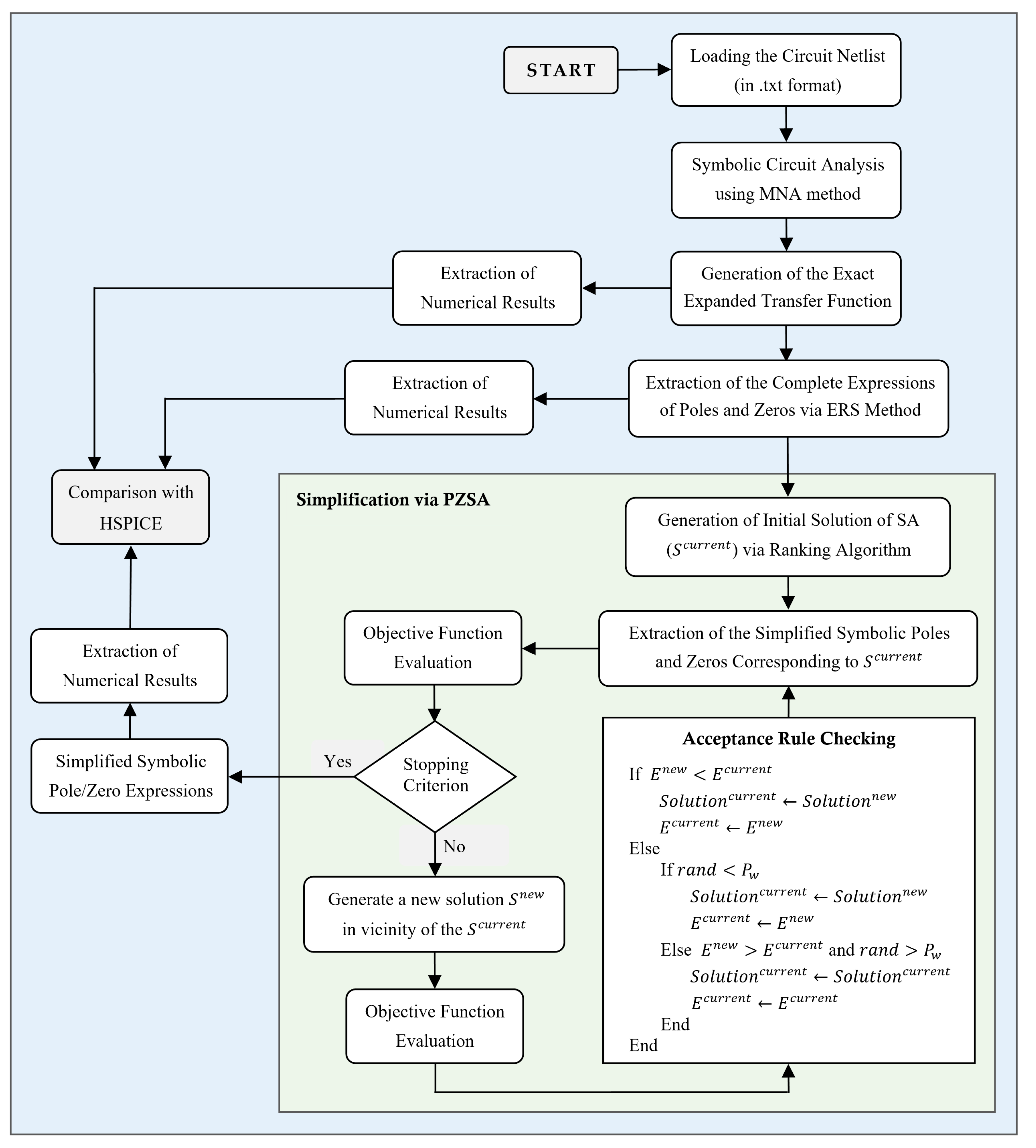
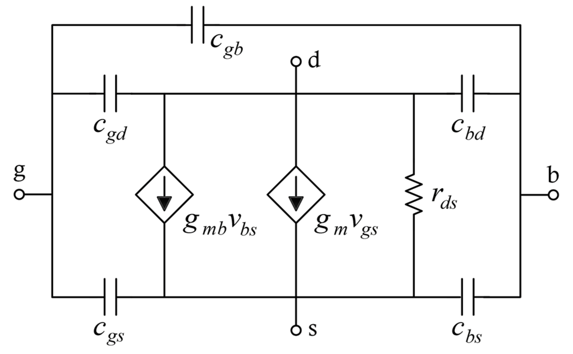
3.1. Symbolic Pole/Zero Extraction via ERS
After the netlist pre-processing, the circuit is solved using MNA [
1], and consequently, the exact symbolic TF is achieved in expanded form. Then, the obtained exact pole/zero expressions are approximately calculated using the proposed ERS method, which is an enhanced version of the traditional root splitting algorithm. Generally, an expanded TF could be converted into the factorized form according to Equation (8), where
is a function of
(real or complex conjugate) zeroes
,
, …,
, and
is a function of
(real or complex conjugate) poles
,
, …,
.
In the ERS algorithm, only poles and zeroes located in the interval [
are extracted, where
and
are the minimum and maximum user-specified frequencies for the pole/zero extraction, respectively. If the user does not specify the frequency range, it is considered as the default range of [
, where
is the unity gain frequency of the exact expression in the nominal point. In the following section, the pole extraction procedure for
is described. By comparing Equations (1) and (8),
can be calculated as:
Assuming
to be dominant and all other poles (typically occurred in OTAs) to be located at much higher frequencies, i.e.,
, the first pole can be split, and thus,
can be approximately written as:
By equating the
coefficients of
in Equation (10) to those in Equation (9), the dominant real pole
can be approximated given as:
Consequently, by assuming the condition in Equation (12), we can simplify the rightmost expression of Equation (10) as Equation (13). By equating the
coefficients of Equation (13) to the same
coefficients in Equation (9), the parameters
can be calculated as Equation (14).
and thus, the leftmost expression in Equation (10) can be expressed as:
The circumstances of
coefficients in the original denominator
, for which Equation (15) is valid, are:
Equation (15) shows that
can be simplified into a product of a first-order polynomial (i.e., first dominant pole) and a high-order polynomial corresponding to other high-frequency poles. In a more general case, assuming the first
poles (
) to be successively dominant in pairs (i.e.,
dominates
,
dominates
, and so on,
dominates
),
can be approximated as follows:
By similar approximations as performed in the previous case,
can be simplified according to:
By equating the
coefficients of Equations (18) and (9), the
first poles are derived as Equation (19). Additionally, the parameters
can be expressed as Equation (20). Thus,
can be simplified into the multiplication of
+1 polynomials:
first-order polynomials (representing the
first poles) and a high-order polynomial, as Equation (21). The conditions on
coefficients of
, for which Equation (21) is valid, can be expressed as Equations (22) and (23).
In the general case, let us extend the above formulations to the case that all the
poles are dominant reciprocally, in which
can be approximated as follows:
Under the assumption that all poles are dominant in pairs (i.e.,
dominates
,
dominates
, and so on), the following conditions are satisfied:
Therefore, the rightmost expression in Equation (24) can be approximated as Equation (26). By equating
coefficients of Equation (26) and Equation (9),
can be approximately expressed as Equation (27), where each pole
can be calculated according to Equation (28).
The interesting point is that all poles are derived from
coefficients of the denominator of the transfer function. The above formulations operate under the assumption that all poles are real. In other words, the approach fails for closely spaced or complex conjugate poles. Therefore, the method should be extended to cases where two consecutive poles are located in a cluster. Assuming that
and
constitute a pair of poles (real or conjugate), they remain split off in the expression
and can be expressed via a second-order polynomial
, where
and
can be calculated as follows:
The condition for which the poles
and
are real is
. If the condition has been satisfied, the real poles
and
can be expressed as Equation (30). Otherwise, these poles can be represented as complex conjugate poles according to Equation (31).
It should be emphasized that all the above formulations could be used to extract simplified zeroes
from the numerator
of the expanded TF. In ERS, the pole
(or zero
) can be separated using Equation (27) if the conditions in Equations (32) and (33) are met, where
(
) is the absolute of the numerical value of
-th pole (
-th zero) extracted via the ERS method and
(
) is the absolute of the
-th pole (
-th zero) of the exact function of Equation (1). These are numerically achieved by the calculation of the roots of the transfer function.
(
) refers to the set of poles (zeroes) which are in the range of the interval [
. Additionally,
is a pre-determined constant parameter used to specify the maximum allowable root displacement for each ERS root compared with the exact one.
The ERS pole/zero extraction method comprises evaluation and extraction steps. In the evaluation step, all poles and zeroes within the interval [
are assumed to be reciprocally dominant. Thus, their ERS values are numerically obtained according to Equation (27). In the extraction step, the conditions of Equations (32) and (33) are checked for all extracted poles and zeroes. Then, each pole (zero) that has satisfied the mentioned condition can be symbolically extracted according to Equation (27). Otherwise, a pair of real or complex conjugate poles (zeroes) remains split off, and the condition
is checked for them. If the condition has been satisfied, the poles (zeroes) are a pair of real poles (zeroes) and can be calculated by Equation (30); otherwise, they are considered as complex conjugate poles (zeroes) which are extracted by means of Equation (31). To gain further insight into the details of the ERS method, the pseudo-code of the symbolic pole/zero extraction method is provided in Algorithm 1.
| Algorithm 1. Symbolic Pole/Zero Extraction using ERS |
| Inputs: |
| Symbolic exact expanded transfer function |
| Numerical values of the circuit parameters in the nominal point |
| ) |
| Output: |
| Symbolic expressions of poles and zeros |
| Numerical Analysis: |
| 1. ) |
| 2. Numerically evaluate the exact expanded transfer function in the nominal point |
| 3.
|
| 4. ) by their magnitude |
| Extraction of Symbolic Zeros: |
| 5.
|
| 6. Numerically estimate the position of zero j as |
| 7.
|
| 8.
|
| 9. else |
10. in one cluster
11. |
| 12.
|
| 13.
|
| 14.
|
| 15. else |
| 16.
|
17. end if
18. end if
19. end for |
| Extraction of Symbolic Poles: |
| 20.
|
| 21.
|
| 22.
|
| 23.
|
| 24. else |
25. in one cluster
26. |
| 27.
|
| 28.
|
| 29.
|
| 30. else |
| 31.
|
32. end if
34. end if
35. end for |


