Abstract
Community detection remains a challenging research hotspot in network analysis. With the complexity of the network data structures increasing, multilayer networks, in which entities interact through multiple types of connections, prove to be effective in describing complex networks. The layers in a multilayer network may not share a common community structure. In this paper, we propose a joint method based on matrix factorization and spectral embedding to recover the groups not only for the layers but also for nodes. Specifically, the layers are grouped via the matrix factorization method with layer similarity-based regularization in the perspective of a mixture multilayer stochastic block model, and then the node communities within a layer group are revealed by clustering a combination of the spectral embedding derived from the adjacency matrices and the shared approximation matrix. Numerical studies show that the proposed method achieves competitive clustering results as the number of nodes and/or number of layers vary, together with different topologies of network layers. Additionally, we apply the proposed method on two real-world multilayer networks and obtain interesting findings which again highlight the effectiveness of our method.
Keywords:
community detection; multilayer network; layer similarity; mixture multilayer stochastic block model MSC:
05C82
1. Introduction
Network analysis has emerged in many areas of research and applications, from sociology and ecology to economics [1,2]. For networks, nodes represent the entities of interest, and connecting edges represent the specific relationship that exists among nodes. As the complexity of real datasets increases, various interactions among the elementary components of these systems have emerged. For example, people may contact each other as workmates in a company and as friends on Facebook; different countries may trade in a variety of products. Traditional monolayer networks, which record only one type of interaction between nodes, are less capable to describe the multiple modes of interactions encountered and to understand the topology of the real datasets precisely. Fortunately, several network models have been in existence as various extensions of monolayer networks. One such example are the multilayer networks in which multiple modes of interactions are considered and each specific interaction forms a layer [3]. In this paper, we focus on the multilayer networks with layers sharing a common set of nodes and without inter-layer edges [4].
Community detection is a fundamental issue when analyzing network data. For monolayer network, community detection aims to cluster nodes into communities, and thus there exist more edges connecting nodes in the same community and fewer edges joining nodes across communities [5]. The community detection problem has significant applications due to the fact that entities in a community are likely to share common properties; for example, people in a community may come from the same place and/or they may share other similar interests [6]. Thus, revealing the community structure in a network can provide a better understanding of the overall functioning of the network. There exists a substantial volume of research about community detection techniques on monolayers, such as probabilistic methods [7,8] and criteria-based approaches [9,10]. For a comprehensive review of these works we refer to [11].
The community detection methods originally proposed for monolayer networks can be used directly to analyze multilayer networks in two ways. One way is to aggregate the layers into a graph and then apply traditional community detection methods on the aggregated network [12,13]. The other way is to use the traditional community detection methods on each layer independently and the clustering results are then merged [14,15]. Several other researchers have also proposed community detection methods for multilayer networks, including probability models [16,17,18,19], spectral methods based on various versions of aggregation adjacency matrices or Laplacian matrices [20,21], matrix factorization methods [22] and criteria based methods such as minimizing a squared objective function or maximizing a modularity function [23,24,25]. Most of these methods aim to detect communities that are common across layers and ignore the inhomogeneous nature of network layers. However, for many real multilayer networks, different layers may have different community structures, and some of the layers are interdependent while others are not. For instance, in an international trade multilayer network in which products represent layers and countries are nodes, the trade patterns among countries related to processed foods may be different from those related to unprocessed foods; on the other hand, the trade activities among countries related to different processed foods may be similar. These findings suggest that we should jointly find groups for layers and assign community memberships to nodes for each layer group.
A few recent works have focused on addressing the community detection problem in inhomogeneous multilayer networks. For example, Ref. [26] introduce a multilayer SBM which clusters layers into groups, the so-called strata, and assume that layers in each strata share a common community structure; Ref. [27] introduce a common subspace independent-edge multiple random graph model allowing a shared latent structure across layers, being layer-specific in each layer, and propose a joint spectral embedding of adjacency matrices to simultaneously estimate underlying parameters for each layer; Ref. [28] investigate the so called “Mixture MultiLayer Stochastic Block Model” (MMLSBM) and propose a regularized tensor decomposition to reveal the communities for the layers and nodes. Ref. [29] propose an alternating minimization algorithm(ALMA) that simultaneously recovers the layer partitions and node partitions. Although the methods for finding layer groups in the mentioned works are a bit different, given the layer groups, these works apply classical cluster methods either on the aggregated adjacency matrices or an estimated matrix of that layer group to find the node assignments. More related works we refer to are [30,31,32].
In this work, we are interested in inhomogeneous multilayer networks under the mixture multilayer stochastic block model (MMLSBM) setting. We consider a two-step procedure to detect the layer groups (between-layer clustering) as well as the node communities within a layer group (within-layer clustering). Unlike commonly used methods that describe the multilayer networks using tensor-wise data in the literature, we instead use the vectorization of the model. This technique can reduce the systematic errors due to the improper setting of parameters in the estimation of the tensor approximations. A combination of the Matrix Factorization and Spectral Embedding method (MFSE) is proposed to handle the joint community detection problem. The present paper makes the following contributions. First, under a vectorized perspective, we propose a matrix factorization based method to recover the layer communities. Moreover, since layers that are very structurally similar are more likely to belong to the same group, we integrate layer similarity regularization into the matrix factorization based objective function. Under the MMLSBM setting, each layer can be described as a stochastic block model (SBM) model and two layers have the same connection probability matrix once they belong to the same layer community. From the least squares perspective, the underlying membership matrix C of the layers is optimized by minimizing the objective function , where is a vectorized version of the adjacency tensor and the l-th row of matrix Q can be treated as the potential representation of the l-th layer community and is the regularization term. Subsequently, we employ the spectral embedding method to recover the node communities in each layer group. For a given layer group, we simultaneously apply the spectral embedding on the adjacency matrices and on the shared structural matrix derived from Q in that group. The final node latent representations are a combination of two types of spectral embeddings. Then, classical clustering methods can be carried out on the joint spectral embedding to search the node assignments. In addition, an efficient singular value decomposition is used to give a recommended value of the number of layer groups as well as the number of node communities in each layer group.
2. Model Framework
2.1. Notations
For a matrix A, let be the Frobenius norm and denote its transpose by . Let and be the i-th row and j-th column of a matrix A, respectively. Denote the Kronecker product of the matrices of matrices A and B by . Some more notations used throughout this paper are collected in Table 1.

Table 1.
Notation definitions.
2.2. Discussion of the Framework
We consider a multilayer network with L layers on the same set of n nodes. For the l-th layer, denote its adjacency matrix by , where if the nodes i and j are connected and otherwise, further, if the l-th layer is undirected and otherwise.
In the MMLSBM setting, are independent Bernoulli random variables with and . The probability matrices give a tensor form . In this paper, we assume that the probability connection tensor can be partitioned into groups. In particular, there exists a label function and a corresponding clustering matrix such that
where is the connectivity matrix satisfying . We aim to recover the network groups as well as the within-layer community assignments .
2.2.1. Between-Layer Cluster
Methods
Adopting the vectorized versions of and , it follows from [33] that
Denote and recall that C is the membership matrix of the layers, i.e., for , if and 0 otherwise. We thus rewrite Equation (1) as
where can be considered as the shared structure matrix of M layer groups.
Similarly, we introduce the matrix . Note that can not be observed directly but can be; combining Equations (1)–(3) and from the perspective of the least-squares method, we propose to estimate the potential layer cluster matrix via the following objective function
In the estimation step, we relax the restrictions on C, i.e., if layer l belongs to group m, and impose the non-negativity together with on C. For the non-negative feature of the matrices and , we can solve the optimization problem of Equation (4) by a nonnegative matrix factorization method.
Intuitively, the layers with high pairwise structural similarity tend to be partitioned into a group. Some effort has been devoted to designing various kinds of indices to measure the similarity between layers [34,35]. In this paper, we use the Pearson linear correlation coefficient to quantify the degree of correlation between two layers l and m [36]. The Pearson correlation coefficient is defined as
where represents the mean degree and is the standard deviation of the layer . There is no doubt that . The closer is to 1 (), the more positively (negatively) correlated the two layers are. Additionally, layers l and m are almost linearly independent if closes to 0.
Above all, a layer similarity based regularization is defined as
where is the Pearson linear correlation and represents the l-th row of matrix C. A simple calculation leads to the following matrix format of Equation (5)
where is the trace function, is the layer similarity matrix and stands for the Laplacian matrix of the layer similarity matrix. is a diagonal matrix representing the degree matrix of S.
By integrating the regularization Equation (6) into Equation (4), we now formalize the between-layer cluster problem as a non-negative matrix factorization problem with layer similarity regularization:
where is a trade-off parameter for the regularization term. In this paper, for , we set the entities which are less than 0 to 0, and choose the parameter in Equation (7) by the cross validation method.
Updating Rules
Note that is not convex with respect to C and Q together; it is thus difficult to find the global minimum of the loss function. To this end, an iterative algorithm is adopted to pursue the solution of Equation (7). In addition, we introduce Lagrange multipliers and for the non-negative constraints on C and Q, respectively. Then the objective function Equation (7) is rewritten as
After that, for and , we multiply by and on both sides of Equations (11) and (12), respectively. Since the KKT conditions imply that and , we obtain the optimal solutions of and as follows:
and
Now, we can recover the communities of network layers by applying K-means algorithm on the rows of . For each m, the estimated represents the shared structural information of layers in the m-th layer group; we transform into M separate matrices. Specifically, for , we consider matrices given by
We stress that represents the shared behavior of node i in the m-th layer group.
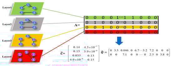
A toy example is further used to describe the procedure of Equation (7). As shown in Figure 1, the simple multilayer network consists of four layers and five nodes. Each row of the matrix represents the vectorized version of the adjacency matrix related to the layer. Applying the updating rules in Equations (13) and (14), we obtain the estimated layer membership matrix and the estimated shared structure information matrix . After that, we use K-means on to obtain the layer groups. Then, by Equation (15), we construct two matrices and based on two rows of , respectively. Each constructed matrix is treated as the potential representation of the related layer group.
2.2.2. Within-Layer Community Detection
Given the layer membership matrix and the shared structure matrix , the issue that we focus on is how to use the structural information within a layer to detect node assignments. Refs. [28,29] applied a classical clustering method either on the aggregated adjacency matrices or an estimated embedding matrix associated to that layer group. To better describe the consistent topology structural across layers within a layer group, we propose to use an aggregated spectral embedding derived from both the observed adjacency matrices in that layer group and of the shared on the task of clustering nodes within a layer group.
Once the group layers are fixed, we average the adjacency matrices in the m-th group as . Then, a standard spectral embedding method is applied on . We list the detailed steps below.
- (Sa):
- Calculate the graph Laplacian
- (Sb):
- Find orthonormal eigenvectors corresponding to the eigenvalues that are largest in absolute value of and put them in a matrix .
- (Sc):
- Form the normalized version by normalizing each row of to have unit length. Then, is considered to be the spectral embedding derived from .
Following the steps (Sa)–(Sc) of the spectral embedding, we are coming to find the embedding representations of nodes from . Denote the graph Laplacian by and the corresponding normalized embedding matrix by .
Based on the above, for the m-th layer group, we add the node representations obtained in with the to obtain extended node representations:
The within-layer community detection is then carried out by applying a K-means algorithm on . Up to now, we formalize a two-step community detection method for multilayer networks based on Matrix Factorization and joint Spectral Embedding (MFSE) which is outlined as Algorithm 1.
Remark 1
(Initializations of C and Q). It is known that random initializations may lead the algorithms into non-informative local minimals. The Pearson correlation matrix S illustrates the structural similarity among layers and thus it can provide a glancing estimation of the membership of the layers. Here, we apply K-means on the layer similarity matrix S and take the centers returned by the K-means algorithm as the initialization of C. In our proposed objective function, each row of Q stands for the potential representations of nodes in a specific layer group, following the way of initializing C; after carrying out K-means on , the initialization of Q is given by the centers returned by the K-means algorithm.
Remark 2
(Pre-determination of M and ). Much work has been carried out for determining the number of communities in the community detection problem ([37,38]), either by maximizing specific objective function or searching all candidates. Among these, the eigengap heuristic method proves to be effective in applications ([39,40]). In this paper, we select the number of layer groups M and number of node communities of the m-th layer group by the eigengap heuristic method. For M, we compute the eigendecomposition of the layer similarity matrix S and then rank the eigenvalues . In practice, there is usually a significant drop between and and we set the number of layer groups as M.
Once the layer groups are fixed, we first obtain the averaged adjacency matrix in the m-th layer group and then apply eigen-decomposition on . After that, is chosen as the number of communities if the eigenvalue is relatively larger than , i.e., the gap between and is much greater than those of other adjacent eigenvalues.
| Algorithm 1 MFSE Algorithm |
| Input: The adjacency matrices ; number of layer groups M; number of the node groups ; tuning parameter . Output: The network groups and the within-layer node communities . Algorithm:
|
3. Theoretical Guarantees
Some additional assumptions are required to analyze the convergence issues. We collect them as follows:
- (A1)
- for ;
- (A2)
- with representing the -th largest eigenvalue of ;
- (A3)
- cluster of layers and local communities balance condition: there exist positive constants such that
Note that Assumption (A1) restricts the sparsity of the network, Assumption (A2) requires that the -th eigenvalue of is not too small and Assumption (A3) is the so-called balanced network condition and is very common in the problem of community detection ([41]).
We need to obtain the estimators and of and based on the observed . First of all, we give a theoretical result on the consistency of the estimators from the objective function . We denote the estimators in the iteration by .
Theorem 1.
converges to a critical point of .
The proof of Theorem 1 is given in Appendix A.
We denote by the permutation function of . Given the true partition of the network layers and the estimated partition , the misclassfication error rate of between-layer clustering can be defined as
Theorem 2.
Suppose that Assumption (A3) holds, there exists a sufficiently small function depending on n and L such that the between-layer clustering error satisfies , where is a positive constant depending on ε.
The proof of Theorem 2 is given in Appendix B.
For the m-th layer group, the cluster centroids sought by K-means algorithm are defined as , satisfying . Let
be the set of misclustered nodes, where represents the parameter centroid corresponding to the i-th node while is the estimated centroid, and is an orthonormal rotation.
Theorem 3.
Assume that the smallest eigenvalue of is larger than and Assumptions (A1)- (A2) hold. There exist constants and for any , with probability at least ; the proportion of misclustered nodes in the m-th layer group satisfies .
The proof of Theorem 3 is given in Appendix C.
4. Experiments
In this section, we assess the performance of the proposed MFSE method through simulated and real-world multi-layer networks. For synthetic multilayer networks, we compare our method with the TWIST method ([28]) and the ALMA method ([29]). Specifically, TWIST focuses on the MMSBM model and applies Tucker decomposition on the observed adjacency tensor to obtain its low-rank approximations. TWIST finds both the global and the local memberships of nodes, together with the memberships of layers. ALMA is an alternating minimization algorithm which aims at revealing the layer partition as well as the node partitions. We remark that both MFSE and ALMA aim at recovering the community assignment of layers together with the nodes. To make the comparison fair, all three competitive methods are only dedicated to detecting the layer partition and the node partition which are also named as “between-layer clustering” and “within-layer clustering”, respectively. For both synthetic multilayer networks and real-word networks, the between-layer clustering error is assessed by (Equation (17)) and the proportion of misclassified nodes within layers (the within-layer clustering error) is evaluated by (Equation (18)).
4.1. Simulation Study
In this part, we test our method on synthetic multilayer networks. We carry out three simulations to evaluate the performance of the proposed method by varying the number of layers L, the number of nodes n and network sparsity parameter , respectively. The clustering results of all methods in three simulations averaged over 500 replications. Below, we elaborate on each of the simulation scenarios.
The purpose of the first simulation is to examine the ability of the proposed method to discover both layer and node clusters as the number of nodes n varies. Imagine a MMLSBM with layers, layer groups and node communities for each layer group. The underlying community assignments of layers and nodes are generated by the multinomial distributions with equal class probabilities for the layers, and for the nodes within a layer group. For completeness, we take into account both assortative and disassortative SBM models ([42]) in the tests. A SBM model is assortative if and disassortative if for , with representing the connection probability ([41]). We set the connection matrices for three layer groups as
where and . Notice that values of govern the strength of the assortative (disassortative) feature of the network. Roughly speaking, the network is assortative if and disassortative if , and the community structure becomes obscure as closes to 1. We increase the number of nodes n from 40 to 400 and record the between-layer clustering error results and within-layer clustering error results of three methods in Figure 2a,b. As expected, both types of errors rates for all three methods decrease substantially as n becomes large, implying the effect of number of nodes on clustering errors. As , the plots demonstrate that MFSE always achieves superior or comparative performances in both between-layer and within-layer clustering.
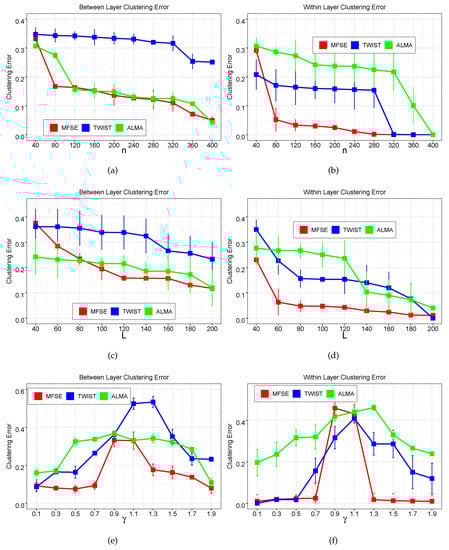
Figure 2.
(a,b) Between-layer clustering results and within-layer clustering results returned by three methods as the number of nodes n increases; (c,d) Between-layer clustering results and within-layer clustering results returned by three methods as the number of layers L increases; (e,f) Between-layer clustering results and within-layer clustering results returned by three methods as varies. Each data point shows the average result and the error bar determines the range of one standard deviation from the average.
In the second simulation, we evaluate the performances of three methods as the number of layers varies. The generated MMLSBM is similar to that in the first simulation except is fixed. We set the number of layers L to increase from 40 to 200. The clustering errors are reported in Figure 2c,d. For all methods, both types of errors decrease as L increases, which is consistent with the theoretical results of these methods. Specifically, for between-layer clustering, MFSE outperforms TWIST and ALMA once , and MFSE continues to obtain superior results for the within-layer clustering.
The last simulation studies the impact of parameter which controls the ratio of the connection probabilities of the inter-groups of nodes versus intra-groups of nodes. The settings are the same as previous simulation scenarios except and are fixed. We set , and the performances of all methods on two types of clustering with increasing from 0.1 to 1.9 are investigated. The results of this comparison are presented in Figure 2e,f. Notice that the smaller the , the more pronounced the within-group and between-group distinction becomes. Additionally, the larger (>1) indicates the stronger disassortative feature of the network. Further, the within-layer clustering becomes harder when closes to 1, which also makes the between-layer clustering difficult. The performances of the three methods in Figure 2e,f agree with those findings.
In summary, for between-layer clustering, the proposed method MFSE achieves better results in all parameter settings and ALMA almost gives the second best results. For within-layer clustering, MFSE still gives superior or comparable performances in different settings. We claim that TWIST works notably even in the cases where the between-layer errors are higher than those of ALAM. This could be due to the fact that TWIST recovers the node partitions by clustering the adjacency matrices in that layer group, while ALAM clusters the low-rank approximation of the adjacency tensor in that layer group which may leave out some direct structure information. We use both direct adjacency matrices and the low-rank approximations to reveal the node memberships within a layer group, which makes our method more effective in various model settings.
4.2. Real-World Network Data
In this section, we demonstrate the merits of MFSE in community detection on two real-world multilayer networks.
4.2.1. FAO data
The data are collected from the Worldwide Food Trading Networks data that are available at https://www.fao.org/faostat/en/#data/TM. The data was collected since 1986 and the last update was given in 23 December 2022. In our analysis, the data was accessed on 1 January 2010, before 31 December 2010. The dataset contains export/import trading among 245 countries/regions for more than 300 products. In the multilayer network, layers represent different types of commodities and nodes represent countries. Two countries have a link if there exist import/export relationships of a product between them. We convert the original directed and weighted networks to undirected and unweighted ones by ignoring the directions and weights. We first remove the layers with links less than 1135 (the third quartile) and retain the layers with average degree greater than 10 (the second quartile). Finally, we choose the countries that are active in trading at least 90% of the selected products, reducing a multilayer network consisting of 46 layers and 100 nodes.
Subsequently, we use Algorithm 1 to recover the partitions of layers (products) and nodes (countries) of the multilayer network. By applying the eigengap heuristic method, we choose and record the between-layer clustering results in Table 2.
Table 2.
Between-layer clustering results obtained by MFSE.
From Table 2, we see that the first layer group consists mostly of solid and liquid beverage products as well as processed food products with a certain shelf life, and the second group contains mostly cereals and raw materials for food products, together with processed food products with a long shelf life.
Applying the eigengap heuristic method again, we choose , which is consistent with the number of continents (Africa, Americas, Asia, Europe, and Oceania) and can be considered as a natural partition of countries. Figure 3 shows the node communities recovered by MFSE. We have the following comments: (1) for both layer groups, there exist close trading activities among some developed and developing countries in Asia and Oceania, for example, China, Japan, Australia, New Zealand, etc, see Community 1 in Figure 3a,b, respectively; (2) for the products in group 1, since North America and Europe are not far apart by ocean transportation, countries in these two regions have more continual demands for trade than the countries in the Americas which have a longer shipping distance, please refer to Communities 2 and 3 in Figure 3a; (3) for the products in group 2, the considerable shelf life of some products allows for close trade among countries with long marine transportation distance, such as among countries in North America and South America (Community 3 in Figure 3b); (4) the countries in Southeast Europe (Community 4 in Figure 3a,b, respectively) have their independent trade patterns regardless of the types of products, probably due to the Free Trade Agreement which was carried out in 2006.
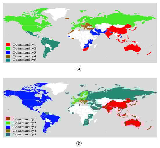
Figure 3.
(a) Node communities found in layer group 1 by MSFE; (b) Node communities found in layer group 2 by MSFE.
4.2.2. AU-CS Network
The network is constructed from a dataset that describes five online and offline relationships including Facebook, leisure, work, coauthor and lunch among 61 employees of a university research department ([43]). The employees are represented by nodes and one specific relationship is represented by one layer, together with links standing for an existing relation between nodes. Thus, a five-layer multilayer network with 620 edges is formed. As a pre-processing step, we computed the eigenvalues of the graph Laplacian based on the layer-similarity matrix and chose by eigengap heuristic. After that, by using the eigengap heuristic method again, we chose as the numbers of node communities in two layer groups, respectively. We apply Algorithm 1 on the data and list the between-layer clustering result in Table 3. The intuition of these layer partitions is that the employees have a natural co-occurrence of work and lunch interactions as colleagues; for example, they may work together and have lunch together in the canteen. Simultaneously, it is natural to group together the online/offline relationships based on personal/research interests.
Table 3.
Between-layer clustering results obtained by MFSE on AU-CS network.
Then, we investigate the within-layer clustering results. Unlike the FAO data, we may not explain intuitively the node partitions and have no idea about the groundtruth communities. For completeness, we use the density metric to evaluate the quality of the clustering method. The density at the l-th network layer is defined as follows:
where, for the l-th layer, and represent the i-th node, the k-th node community and the edge set, respectively. Additionally, to make the results comparable, we introduce a standard Spectral Clustering based method (SPC-Mean) in the literature which uses the Mean adjacency matrix to recover the node communities. We record the densities of each layer returned by the proposed MFSE method and SPC-Mean method in Table 4. We further plot the adjacency matrix of each layer returned by MFSE (Figure 4) where nodes are arranged according to the community labels. Table 4 shows that MFSE gives highly competitive densities for all layers on the AU-CS network and Figure 4 implies that the connection patterns of the first three layers are significantly different from those of the remaining two layers.
Table 4.
Densities obtained by MFSE and SPC-Mean on each layer of AU-CS network.
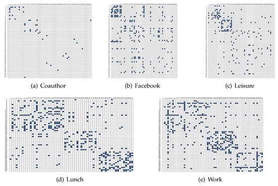
Figure 4.
(a–e) Adjacency matrices of five layers on AU-CS network with nodes arranged according the community labels obtained by MFSE.
5. Conclusions
In this paper, we propose a matrix factorization and spectral embedding based community detection method for multilayer networks. The proposed method recovers the layer groups by clustering the low-rank approximate of a vectorized version matrix derived by the adjacency matrices. After that, the node communities within a layer group can be recovered by both the observed adjacency matrices and a shared structural matrix in that layer group. We give the theoretical guarantees of the method and the simulation results confirm the fact that the proposed method performs efficiently under different model settings. Notice that the layers of networks may have various degrees of sparsity in many real applications; it is thus of interest to extent our method to more sparse scenarios in future studies. Another direction worth exploring is where one can generalize the matrix factorization-based representation incorporating node attributes to extract communities in multilayer networks.
Author Contributions
Conceptualization, F.T.; methodology, F.T.; software, X.Z.; validation, X.Z.; formal analysis, X.Z.; investigation, F.T.; resources, C.L.; data curation, C.L.; writing—original draft preparation, C.L.; writing—review and editing, C.L.; visualization, C.L.; supervision, C.L.; project administration, F.T.; funding acquisition, F.T. and X.Z. All authors have read and agreed to the published version of the manuscript.
Funding
This work is supported by the National Natural Science Foundation of China (12201235, 11971214), Natural Science Foundation of Anhui Province (2108085QA14), the Excellent Young Talents Fund Program of Higher Education Institutions of Anhui Province (gxyqZD2022044) and Qinglan Project of Jiangsu Province.
Data Availability Statement
Not applicable.
Acknowledgments
The authors would like to thank the editor, associate editor and referees.
Conflicts of Interest
The authors declare no conflict of interest.
Abbreviations
The following abbreviations are used in this manuscript:
| MFSE | Matrix factorization and spectral embedding method |
| MMLSBM | Mixture multilayer stochastic block model |
| TWIST | Tucker decomposition with integrated SVD transformation |
| ALMA | Alternating minimization algorithm |
Appendix A
The proof of Theorem 1 is based on the following lemmas and the Kurdyka–Lojasiewicz property.
Lemma A1.
There exists a constant such that for
Proof.
Since and the sequence of of is monotone decreasing, the result is obtained. □
Lemma A2.
For each , it holds that where and is the largest eigenvalue of .
Proof.
Denote . For each , we have
where ⊗ is the Kronecker product of two matrices.
Similarly, we have
□
Lemma A3.
For any and , it holds that , where .
Proof.
It follows from Equation (11) that
On the other hand,
Let be a point and a point set, respectively. Define as the shortest distance between x and Denote the class of all concave and continuous functions satisfying: (1) ; (2) is continuous differentiable on and (3) for all . Now, we are presenting the Kurdyka–Lojasiewicz (KL) property.
Definition A1.
(Kurdyka–Lojasiewicz (KL) property [44]) Let be a proper lower semicontinuous function. For if there exists an , a neighborhood of and a function such that for all , it holds that
then κ satisfies the KL property at . Further, if κ satisfies the KL property at each point in , we then call κ a KL function.
Proof of Theorem 1.
The proof of Theorem 1 is based on the sufficient conditions provided by Lemmas A1–A3 and the KL property in Definition A1. An analogous analysis of convergence about the integrative matrix factorization problem was completed in [45]. The proof of Theorem 1 can be conducted according to Theorem 1 in [45]. We omit the details here. □
Appendix B
The proof of Theorem 2 requires the following lemma simplified from [32], which provides an error bound for any -approximate K-means solution.
Lemma A4.
Let with K distinct rows satisfying with γ a positive constant. Let and be an solution to K-means problem with input ; then, the number of errors in is no larger than for some constant depending only on ε.
Proof of Theorem 2.
It follows from Theorem 1 that there exist a sufficiently small function depending on n and L such that Note that with . Combining this fact with Lemma A4, we conclude that the misclassification rate is not larger than □
References
- Girvan, M.; Newman, M.E.J. Communitystructureinsocial and biological networks. Proc. Natl. Acad. Sci. USA 2002, 99, 7821–7826. [Google Scholar] [CrossRef]
- Javed, M.A.; Younis, M.S.; Latif, S.; Qadir, J.; Baig, A. Community detection in networks: A multidisciplinary review. J. Netw. Comput. Appl. 2018, 108, 87–111. [Google Scholar] [CrossRef]
- Kim, J.; Lee, J.G. Community detection in multi-layer graphs: A survey. ACM Sigmod Rec. 2015, 44, 37–48. [Google Scholar] [CrossRef]
- Kivelä, M.; Arenas, A.; Barthelemy, M.; Gleeson, J.P.; Moreno, Y.; Porter, M.A. Multilayer networks. J. Complex Netw. 2014, 2, 203–271. [Google Scholar] [CrossRef]
- Hric, D.; Darst, R.K.; Fortunato, S. Community detection in networks: Structural communities versus ground truth. Phys. Rev. E 2014, 90, 062805. [Google Scholar] [CrossRef] [PubMed]
- Traud, A.L.; Kelsic, E.D.; Mucha, P.J.; Porter, M.A. Comparing community structure to characteristics in online collegiate social networks. SIAM Rev. 2011, 53, 526–543. [Google Scholar]
- Mariadassou, M.; Robin, S.; Vacher, C. Uncovering latent structure in valued graphs: A variarion approach. Ann. Appl. Stat. 2010, 4, 715–742. [Google Scholar] [CrossRef]
- Amini, A.A.; Chen, A.; Bickel, P.J.; Levina, E. Pseudo-likelihood methods for community detection in large sparse networks. Ann. Stat. 2013, 41, 2097–2122. [Google Scholar] [CrossRef]
- Newman, M.E.J. Modularity and community structure in networks. Proc. Natl. Acad. Sci. USA 2006, 103, 8577–8582. [Google Scholar] [CrossRef]
- Karrer, B.; Newman, M.E. Stochastic blockmodels and community structure in networks. Phys. Rev. E 2011, 83, 016107. [Google Scholar] [CrossRef]
- Fortunato, S.; Darko, H. Community detection in networks: A user guide. Phys. Rep. 2016, 659, 1–44. [Google Scholar] [CrossRef]
- Taylor, D.; Caceres, R.S.; Mucha, P.J. Super-resolution community detection for layer-aggregated multilayer networks. Phys. Rev. X 2017, 7, 031056. [Google Scholar] [CrossRef] [PubMed]
- Taylor, D.; Shai, S.; Stanley, N.; Mucha, P.J. Enhanced detectability of community structure in multilayer networks through layer aggregation. Phys. Rev. Lett. 2016, 116, 228301. [Google Scholar] [CrossRef] [PubMed]
- Dong, X.; Frossard, P.; Vandergheynst, P.; Nefedov, N. Clustering on multi-layer graphs via subspace analysis on grassmann manifolds. IEEE Trans. Signal. Proces. 2013, 62, 905–918. [Google Scholar] [CrossRef]
- Tang, L.; Wang, X.; Liu, H. Community detection via hetero- geneous interaction analysis. Data Min. Knowl. Discov. 2012, 25, 1–33. [Google Scholar] [CrossRef]
- Xu, K.S.; Hero, A.O. Dynamic stochastic blockmodels for time-evolving social networks. IEEE J. Sel. Top. Signal Process. 2014, 8, 552–562. [Google Scholar] [CrossRef]
- Han, Q.; Kevin, X.; Edoardo, A. Consistent estimation of dynamic and multi-layer block models. In Proceedings of the International Conference on Machine Learning, Miami, FL, USA, 9–11 December 2015; pp. 1511–1520. [Google Scholar]
- Tang, R.; Tang, M.; Vogelstein, J.T.; Priebe, C.E. Robust estimation from multiple graphs under gross error contamination. arXiv 2017, arXiv:1707.03487. [Google Scholar]
- De Bacco, C.; Power, E.A.; Larremore, D.B.; Moore, C. Community detection, link prediction, and layer interdependence in multilayer networks. Phys. Rev. E 2017, 95, 042317. [Google Scholar] [CrossRef] [PubMed]
- Dong, X.; Frossard, P.V.; Ergheynst, P.; Nefedov, N. Clustering with multi-layer graphs: A spectral perspective. IEEE. Trans. Signal. Proces. 2012, 60, 5820–5831. [Google Scholar] [CrossRef]
- Bhattacharyya, S.; Chatterjee, S. Spectral clustering for multiple sparse networks: I. arXiv 2018, arXiv:1805.10594. [Google Scholar]
- Tang, W.; Lu, Z.; Dhillon, I.S. Clustering with multiple graphs. In Proceedings of the Ninth IEEE International Conference on Data Mining, Miami, FL, USA, 6–9 December 2009; pp. 1016–1021. [Google Scholar]
- Lei, J.; Chen, K.; Lynch, B. Consistent community detection in multi-layer network data. Biometrika 2020, 107, 61–73. [Google Scholar] [CrossRef]
- Mucha, P.J.; Richardson, T.; Macon, K.; Porter, M.A.; Onnela, J.P. Community structure in time-dependent, multiscale, and multiplex networks. Science 2010, 328, 876–878. [Google Scholar] [CrossRef]
- Bazzi, M.; Porter, M.A.; Williams, S.; McDonald, M.; Fenn, D.J.; Howison, S.D. Community detection in temporal multilayer networks, with an application to correlation networks. Multiscale Model. Simul. 2016, 14, 1–41. [Google Scholar] [CrossRef]
- Stanley, N.; Shai, S.; Taylor, D.; Mucha, P.J. Clusteringnetwork layers with the strata multilayer stochastic block model. IEEE. Trans. Netw. Sci. Eng. 2016, 3, 95–105. [Google Scholar] [CrossRef]
- Arroyo, J.; Athreya, A.; Cape, J.; Chen, G.; Priebe, C.E.; Vogelstein, J.T. Inference for multiple heterogeneous networks with a common invariant subspace. J. Mach. Learn. Res. 2021, 22, 6303–6351. [Google Scholar]
- Jing, B.Y.; Li, T.; Lyu, Z.; Xia, D. Community detection on mixture multilayer networks via regularized tensor decomposition. Ann. Stat. 2021, 49, 3181–3205. [Google Scholar] [CrossRef]
- Fan, X.; Pensky, M.; Yu, F.; Zhang, T. ALMA: Alternating Minimization Algorithm for Clustering Mixture Multilayer Network. J. Mach. Learn. Res. 2022, 23, 6303–6351. [Google Scholar]
- Le, C.M.; Levin, K.; Levina, E. Estimating a network from multiple noisy realizations. Electron. J. Stat 2018, 12, 4697–4740. [Google Scholar] [CrossRef]
- Chen, S.; Liu, S.; Ma, Z. Global and individualized community detection in inhomogeneous multilayer networks. Ann. Stat. 2022, 50, 2664–2693. [Google Scholar] [CrossRef]
- Lei, J.; Lin, K.Z. Bias-adjusted spectral clustering in multi-layer stochastic block models. J. Am. Stat. Assoc. 2022, 1–13. [Google Scholar] [CrossRef]
- Gupta, A.K.; Nagar, D.K. Matrix Variate Distributions; Chapman Hall/CRC Press: Boca Raton, FL, USA, 2000. [Google Scholar]
- De Domenico, M.; Granell, C.; Porter, M.A.; Arenas, A. The physics of spreading processes in multilayer networks. Nat. Phys. 2016, 12, 901–906. [Google Scholar] [CrossRef]
- De Domenico, M.; Biamonte, J. Spectral entropies as information-theoretic tools for complex network comparison. Phys. Rev. X 2016, 6, 041062. [Google Scholar] [CrossRef]
- Nicosia, V.; Latora, V. Measuring and modeling correlations in multiplex networks. Phys. Rev. X 2015, 92, 032805. [Google Scholar] [CrossRef] [PubMed]
- Yang, L.; Cao, X.; Jin, D.; Wang, X.; Meng, D. A unified semi-supervised community detection framework using latent space graph regularization. IEEE Trans. Cybern. 2015, 45, 2585–2598. [Google Scholar] [CrossRef] [PubMed]
- Ma, X.; Gao, L.; Yong, X.; Fu, L. Semi-supervised clustering algorithm for community structure detection in complex networks. Phys. A 2010, 389, 187–197. [Google Scholar] [CrossRef]
- Luxburg, V. A tutorial on spectral clustering. Stat. Comput. 2007, 17, 395–416. [Google Scholar] [CrossRef]
- Lu, H.; Sang, X.; Zhao, Q.; Lu, J. Community detection algorithm based on nonnegative matrix factorization and pairwise constraints. Phys. A 2020, 545, 123491. [Google Scholar] [CrossRef]
- Amini, A.A.; Levina, E. On semidefinite relaxations for the block model. Ann. Stat. 2018, 46, 149–179. [Google Scholar] [CrossRef]
- Tang, F.; Wang, C.; Su, J.; Wang, Y. Spectral clustering-based community detection using graph distance and node attributes. Computation. Stat. 2020, 35, 69–94. [Google Scholar] [CrossRef]
- Rossi, L.; Magnani, M. Towards effective visual analytics on multiplex and multilayer networks. Chaos. Soliton. Farct. 2015, 72, 68–76. [Google Scholar] [CrossRef]
- Attouch, H.; Bolte, J.; Svaiter, B.F. Convergence of descent methods for semi-algebraic and tame problems: Proximal algorithms, forward-backward splitting, and regularized gauss-seidel methods. Math. Programm. 2013, 137, 91–129. [Google Scholar] [CrossRef]
- Liu, J.; Wang, J.; Liu, B. Community detection of multi-Layer attributed networks via penalized alternating factorization. Mathematics 2020, 8, 239. [Google Scholar] [CrossRef]
- Lei, J.; Rinaldo, A. Consistency of spectral clustering in stochastic block models. Ann. Stat. 2015, 43, 215–237. [Google Scholar] [CrossRef]
- Binkiewicz, N.; Vogelstein, J.T.; Rohe, K. Covariate-assisted spectral clustering. Biometrika 2017, 104, 361–377. [Google Scholar] [CrossRef] [PubMed]


Disclaimer/Publisher’s Note: The statements, opinions and data contained in all publications are solely those of the individual author(s) and contributor(s) and not of MDPI and/or the editor(s). MDPI and/or the editor(s) disclaim responsibility for any injury to people or property resulting from any ideas, methods, instructions or products referred to in the content. |
© 2023 by the authors. Licensee MDPI, Basel, Switzerland. This article is an open access article distributed under the terms and conditions of the Creative Commons Attribution (CC BY) license (https://creativecommons.org/licenses/by/4.0/).