3.1. Transformer in Federated Learning
This research develops a vision-based privacy-preserving and effective fire detection system to address the security issue of image information leakage in fire detection and to detect fires while protecting privacy. A significant portion of client camera data cannot be made public due to privacy concerns; hence, current solutions suffer from the problem of sparse datasets. Due to the limited amount of the dataset, the high-dimensional input space corresponding to the tiny sample size is sparse, making it challenging for neural networks to discover mapping correlations from it. Training the neural network can so easily result in overfitting. In this paper, generated Gaussian noise is utilized to enhance the model’s robustness and generalization to diverse input, hence facilitating neural network learning.
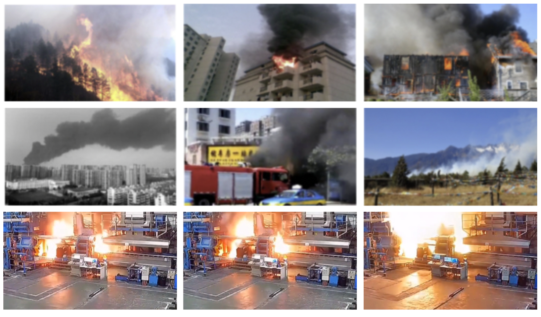
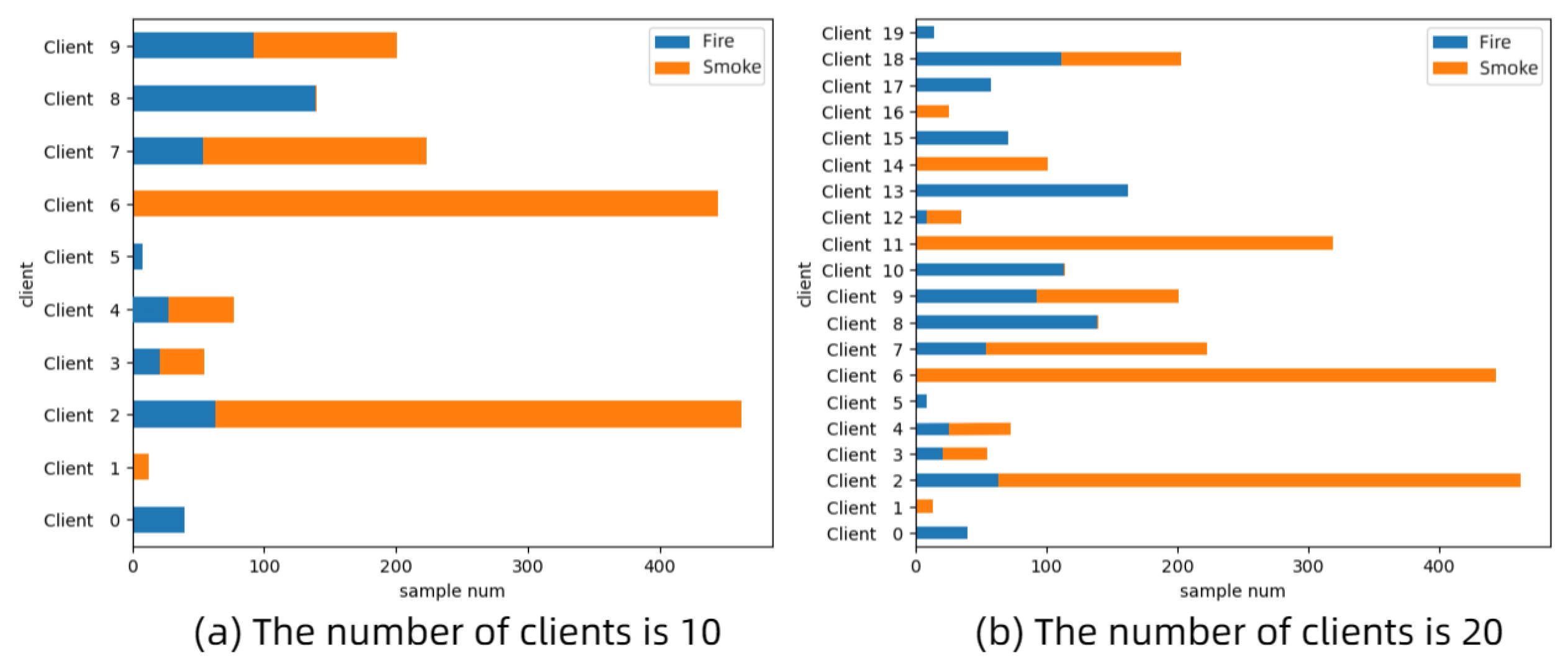
In addition, the objective of federated learning is to train machine learning models using private data from a large number of distributed devices. Data heterogeneity in the scenario of fire detection is generated by factors such as the employment of different cameras, monitored settings, and levels of illumination. Parallel federated learning approaches display unguaranteed convergence and model weight scattering as a result of the spread of training data among numerous clients. Therefore, we employ the transformer instead of a conventional neural network for federated learning to address this issue.
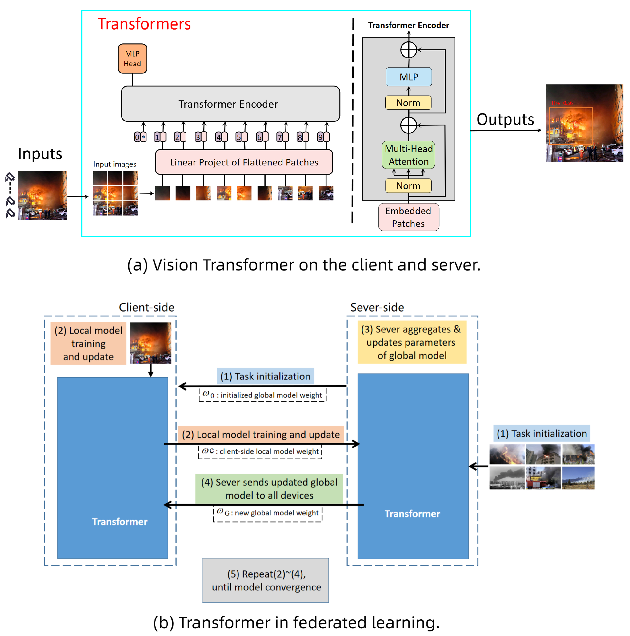
The architecture of our method is demonstrated in the
Figure 1. Transformer, an attention-based encoder-decoder architecture, has revolutionized not only the field of natural language processing (NLP), but also the field of computer vision. The input to the transformer family of models is a sequence of tokens, denoted by
, and this token word embedding is represented by the matrix
. There are stacked multiple layers in the transformer, and the transformer computes the output of the final
lth layer
. The core part of the transformer is the multi-headed attention mechanism, and the computation process of the
h th attention head can be expressed as
Here, and denotes the attention weight of to . They are the Query (Q), the Key (K), the Value (V), and attention (A). Q, K, and V are three different weight matrices by the embedding vector X which is multiplied by 3 different weight matrices , , . Usually there are multiple heads; the number is denoted as , and then the computation result of the multi-head attention mechanism is denoted as , where represents the splicing operation.
In comparison to convolutional neural networks (CNN), visual transformer (ViT) focuses on superior modeling skills to produce an exceptional performance on ImageNet, COCO, and other datasets. The multi-head self-attention (MSA) block, the position encoding block, and the multi-layer perceptron (MLP) block make up ViT’s structural components [
24]. The following are the formulas for ViT.
Prior to the first MSA, the input is added with the position encoding block. LN is the layer-normalization layer. The following is the formulation of the MSA mechanism.
The floating-point operations per second (FLOPs) of MSA and MLP are and , respectively, when the hidden dimension of MLP is by default set to . The ViT with L blocks has FLOPs.
Recent research has shown that replacing traditional neural networks in federated learning with transformer can considerably reduce catastrophic forgetting, expedite convergence, and build superior global models, especially when dealing with heterogeneous data [
23]. The transformer model’s enhanced robustness to heterogeneous data, which significantly reduces the catastrophic forgetting of previous devices during training on various new devices, is the main area of improvement. Visual transformer (ViT) is resistant to a variety of corruptions, a characteristic attributable in part to the self-attention process. Self-attention enhances naturally forming clusters in the token, as confirmed by Zhou D et al. [
25].
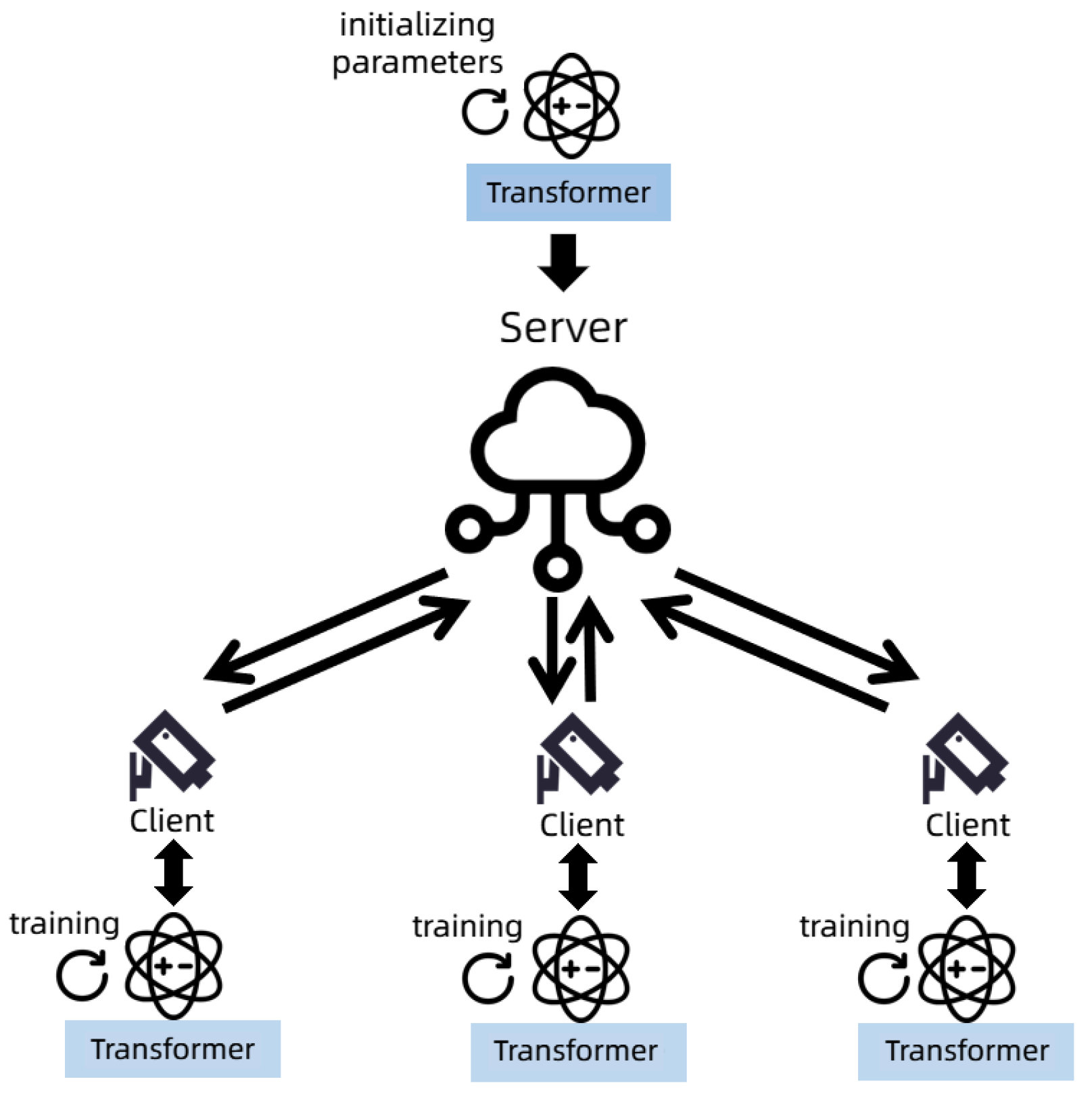
As shown in
Figure 2, it is the improved architecture in this paper. In the federated learning architecture, we use the transformer model to replace the traditional neura network.
Transform is the basic object detection algorithm of the whole system. The main body of a transmission is the parameters of the transformer model. Here are the steps:
- 1.
The server trains first and sends the model parameters to the client;
- 2.
The clients continue training with their local dataset on this basis;
- 3.
The server aggregates and updates parameters;
- 4.
The server distributes the global model to the clients;
- 5.
Repeat, until model convergence.
3.2. Improved Federated Learning Algorithm
Federated learning for edge networks in machine vision-based fire detection systems necessitates interaction with multiple edge nodes. Furthermore, client and server wireless communications are frequently sluggish or unreliable, and bandwidth resources are more limited; so, we wish to reduce the number of client–server communication rounds. The amount of the dataset on each device, however, is less than the total size of the dataset, and the processor speed of the edge device is relatively quick. Consequently, the calculation cost of many model types is typically ignored in comparison to the cost of communication. In this instance, the number of communication rounds is a performance bottleneck for the entire learning framework [
26].
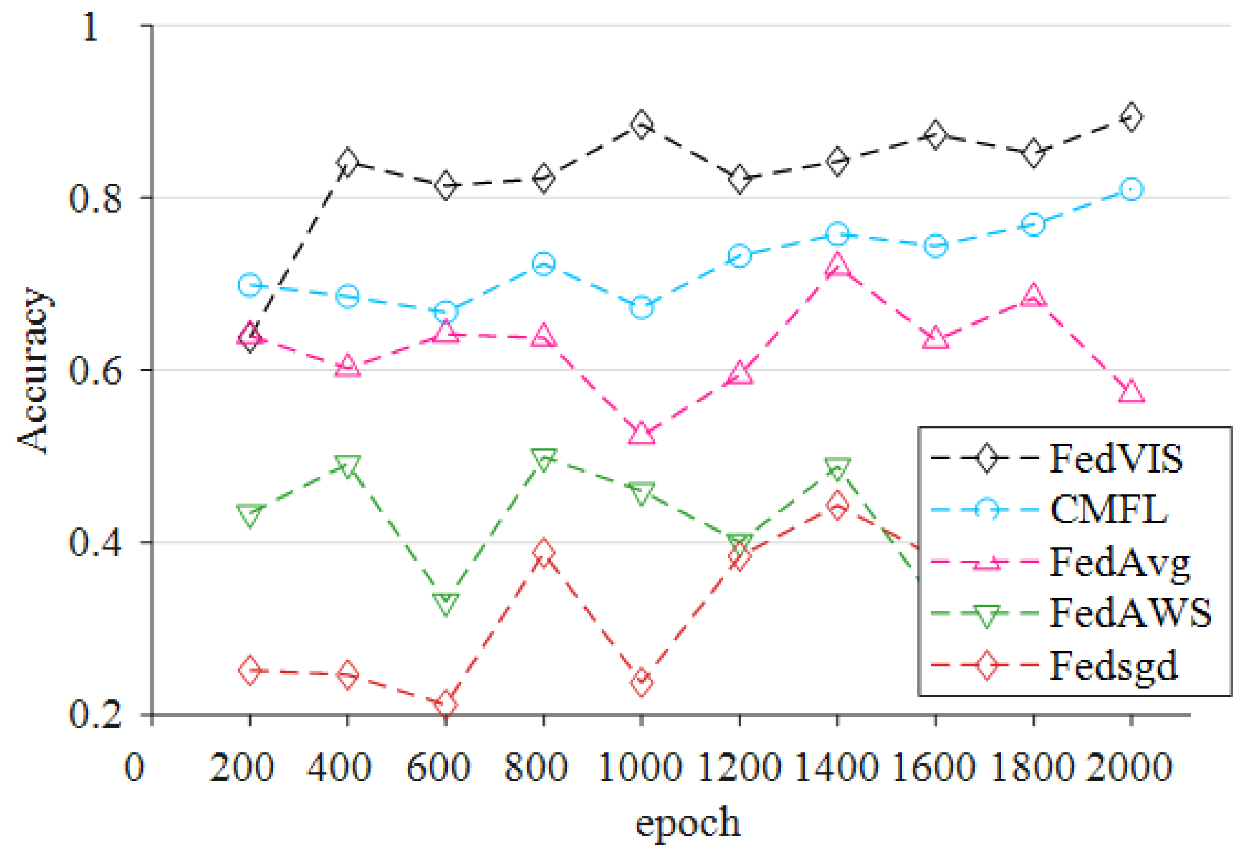
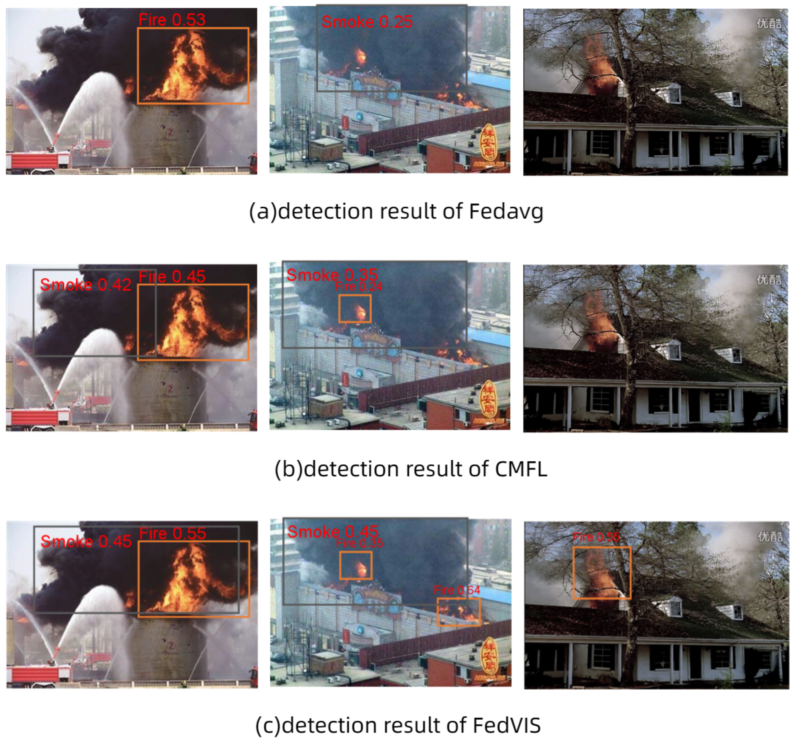
In order to ensure that the correctness of the final global model is not compromised, even if communication costs are saved, this research offers an enhanced federated learning approach called FedVIS. The gradient selection method and the federated dropout algorithm are used to lower the communication cost of federated learning. Furthermore, it reduces the downlink communication overhead between the central server and the client. In addition, it may be effortlessly linked with the uplink communication overhead handling mechanism. It reduces the cost of communication without diminishing the accuracy of the final global model. Simultaneously, the model’s complexity is lowered, hence increasing its generalizability. We selected to upload K gradient values based on the literature cited in [
27]. The criterion for selection is the Pearson product-moment correlation coefficient, which evaluates the association between the global gradient and the client gradient. Then, only the gradient with the highest correlation is uploaded. This allows the gradient value uploaded by the client to be constrained to be closer to the global gradient value. It reduces not only the cost of calculations but also the cost of communication, based on the concept of maintaining model convergence. In addition, it theoretically guarantees model convergence when data are not independent and distributed equally, and it is more durable and stable in heterogeneous federated networks. In addition, in the Federated Dropout algorithm [
28], each client learns smaller submodels, which are subsets of the global model rather than training updates to the complete global model locally. Consequently, the communication burden in federated learning is greatly decreased. Compared to other federated learning algorithms, the FedVIS algorithm has the following advantages:
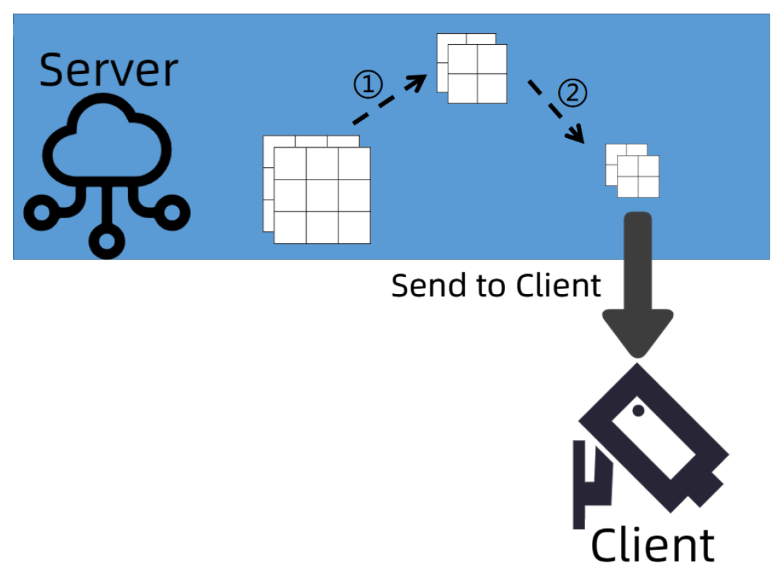
(1) Saving the server-to-client communication overhead. This study introduces the Federated Dropout technique to significantly reduce communication costs. Instead of training the update of the global model locally, each client simply trains the update of a submodel. In the conventional Dropout method, a random binary mask is multiplied with the hidden units in order to reject a percentage of the desired neurons each time training is relayed through the network. Because the mask differs between processes, each process must calculate the gradient relative to a unique submodel. Based on the number of neurons deleted from each layer, these submodels can have varied sizes (structures). To reduce communication overhead in federated learning, we cancel a predetermined amount of activations on each fully linked layer such that all submodels have the same simple architecture.
As shown in
Figure 3, we choose a random activation from each layer to discard, producing a submodel with a 2 × 2 dense matrix.
Therefore, only the necessary coefficients are transferred to the client and repackaged into smaller dense matrices.
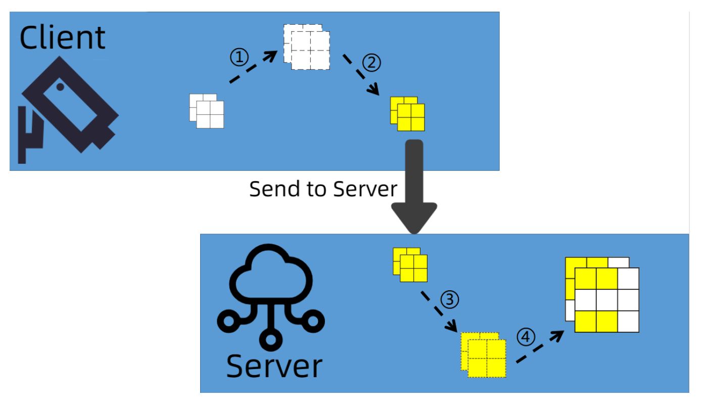
(2) The cost of local computation is reduced further in federated learning. Additionally, the size of client-to-central server updates is decreased, and the local training procedure requires fewer gradient updates. As depicted in
Figure 4, in addition to saving the communication cost from server to client, Federated Dropout also brings two other benefits. First, the scale of client-to-central server updates has also decreased. Secondly, the local training process now only needs to run fewer gradient updates [
28]. At present, all matrix multiplication methods are of smaller dimensions (relative to the full connection layer) or only need to use a few filters (for the convolution layer). Therefore, the use of Federated Dropout further reduces the local computing costs in federated learning.
The client, uninformed of the original model’s design, trains its sub-model and provides its updates; then, the central server maps the updates back to the global model. For the convolutional layer, zeroing out the activation does not result in any space savings; therefore, a portion of the filter is eliminated. Therefore, all current matrix multiplications are of lower dimensionality or employ fewer filters.
(3) Choosing partial gradient uploads for each client will speed up the training. In the Internet context, where the uplink speed is significantly slower than the download connection speed, the interactive communication time is primarily focused on the gradient data upload phase. According to the research [
29], it is shown that 99% of ladder interaction communication is redundant in machine learning models with distributed architecture. These duplicate gradients impose a non-negligible communication burden on the parameter server, which can be substantial. In addition, the data between devices is diverse due to differences in fire monitoring camera models, monitoring conditions, and other aspects. If the gap between each client’s optimized model and the initial global model supplied by the server is too great, the local model will diverge from the original global model. It will slow the global model’s convergence. Based on the FedAvg loss function, LI Tian et al. [
28] developed a proximal term to ensure that the model parameters produced by the client after local training are not too different from the initial server values. In the FedVIS algorithm, only gradients having a high correlation with the global gradient are selected for uploading to the server, thereby further accelerating training and decreasing communication time.
Specifically, the global gradient vector
w is first solved on the server side, and then the Pearson coefficients of
and
can be derived sequentially after the client side calculates the gradient vector
g in each training.
where
is the absolute value of the 1st element of the gradient vector
g and
is the absolute value of the
j th element of the gradient vector
g. The ratio of the covariance and standard deviation of two variables is known as the Pearson correlation coefficient. This coefficient is used to analyze the degree to which two variables are related to one another. Then, all the obtained Pearson correlation coefficients are stored in the array
, and the gradient vector corresponding to the K Pearson correlation coefficients with the largest value are taken to the array
, and only these K gradient vectors are uploaded to the server side. This not only decreases the cost of transmission but also prevents insignificant updates from impacting the use of processing resources and the final detection performance. Algorithm 1 is the final FedVIS pseudo-code designed in this paper.
Algorithm 1 FedVIS
B: local batch size; R: number of server-side iterations; E: number of local iterations; g: gradient vector (indexed by j) computed by the client; v: gradient value threshold; : server-side initialized global gradient vector |
Server global optimization:- 1:
Initialization of all server-side parameters; - 2:
for each round t = 1, 2, … R do - 3:
Server constructs submodels by Federated dropout( ), zeroing a fixed number of activations at each fully connected layer and dropping a fixed percentage of filters at the convolution layer; - 4:
Update all parameters to the client; - 5:
end for
Client local optimization: //execute on chosen client k- 6:
←(divide local client data by size B); - 7:
G = [], TK = [];/*G stores Pearson coefficients , and index ind. stores gradient vectors */ - 8:
for each local epoch i from 1 to E do - 9:
Client computes the gradient vector - 10:
for in g do - 11:
; /*Pearson coefficients , according to Equation ( 9) */ - 12:
Sort G by ; /*Sort from largest to smallest. */ - 13:
end for - 14:
for to K do - 15:
; /* ’s elements are gradient vectors. “ind” is the index of g. */ - 16:
end for - 17:
Upload the gradients in to the server; - 18:
end for
|


