Invoice Discounting Using Kelly Criterion by Automated Market Makers-like Implementations

Abstract

Funding shortages are a persistent issue, particularly for small and medium-sized enterprises (SMEs), and the problem tends to worsen cyclically. The market for factoring and invoice discounting aims to address delays in payment for commercial invoices. These involves sellers present unpaid invoices to financial organizations, typically banks, who provide an advance payment. The implementations of the factoring services without intermediaries in blockchain of the state of the art are all based on the publication on-chain of all the invoices, use know your customer (KYC) mechanisms, and over-collateralize the invoices. This article proposes a new, decentralized approach to lending services that completely eliminates intermediaries and does not require strong KYC, yet it is reasonably resilient. The approach uses liquidity pools and associated heuristics to create a model of risk compensation. In this model, a formula measures the contributed collateral to an invoice and the risk of a late invoice or non-payment, using the Kelly criterion to calculate the optimal premium for funding said invoice in the liquidity pool. The algorithm’s performance is tested in many scenarios involving several invoice amounts, collaterals, payment delays, and non-payment rates. The study also examines premium distribution policies and hack scenarios involving bogus, non-payable invoices. The outcome is a decentralized market that uses the Kelly criterion and is reasonably resilient to a wide range of invoicing scenarios, including 5% non-payment rates and 10% bogus invoices, yet provides a sound profit to liquidity providers. The algorithm’s resilience is enhanced by several premium distribution policies over partially collateralized invoices from 50 to 70%, resulting in optimal premium withdrawal policies every 30 days, making it the first protocol for loanable funds that does not require over-collateralization to be profitable and resilient.

1. Introduction

It is important to study how to improve funding of companies, as [1] exposed a strong positive relationship between access to finance and job growth. Overall, firms with access to a loan exhibit employment growth between 1 to 3 percentage points larger than firms with no access to finance. In the case of SME (Small and Medium Enterprises), they are the top job creators, but they suffer from a lack of funding and late payments to their invoices. No wonder the global market of invoice discounting will grow at a steady rate over the next few years [2]. Invoice discounting represents 10% of banks’ provided credit, a major source of working capital finance globally [3]. It seems it will become even greater in the next crisis, due to their cyclical nature. In particular, invoice discounting is an effective way to help companies troubled by late payments (when invoices are paid in one to three months). Over the recent decades, in the European Union alone, the factoring market has surpassed loans and other forms of funding [3]. Moreover, invoice discounting has another benefit, in that the customer (debtor) is not informed that the supplier (creditor) is being financed. From the suppliers’ point of view, this confidentiality is good for easing negotiations, as they hide the weakness of using working capital finance.

According to [4], small companies in the financial market are not being adequately served, despite the recognition that this market has the potential to meet their liquidity needs. The difficulty lies in assessing the authenticity of the parties involved in the invoice marketplace and determining whether an invoice has already been factored. These challenges make it easy for fraudulent activities, such as double pledging or selling non-existent invoices, to take place. Such fraudulent practices can cause problems for buyers who may be contacted by fraudulent factors demanding payments for invoices that have already been factored by legitimate sellers. Moreover, even in the absence of fraud, paying the invoice to the wrong organization can lead to several problems.

A possible solution to this problem could be a centralized system where all invoices could be stored and verified by interested parties. However, despite the factoring market’s existence for centuries, no such entities have emerged due to the need for confidentiality. Buyers, factors, and sellers are reluctant to share information about past invoices, as disclosing them can work against you for a number of reasons. The study presented in [4] proposes a third-party solution to address the shortcomings of centralized systems. As mentioned in [5], preventing an invoice from being factored twice is a crucial feature of a factoring system. Blockchain technology has the potential to revolutionize various financial processes such as inter-company transactions, procure-to-pay, order-to-cash, rebates, warranties, and financing (including trade finance, letters of credit, and invoice factoring). Recent surveys such as [6,7,8,9,10] suggest that wherever paper-based systems are prevalent, blockchain can offer a promising alternative.

1.1. Invoice Discounting and Factoring

Invoice discounting provides the advantage of accelerating cash flow from customers to suppliers, as suppliers receive advance payments from the bank rather than waiting for customer payment. This allows businesses to invest in growth and expansion. However, faster invoice discounting services need to be provided while preventing double spending and minimizing risk. Blockchain frameworks have the potential to address these issues and transform the invoice discounting process by providing increased transparency and reducing risk for all parties involved, including suppliers, customers, and financial institutions.

Factoring is a financial transaction where a business sells its accounts receivable (i.e., invoices) to a third party at a discount to meet its immediate cash needs. Factoring faces issues related to inter-mediation and trade finance and supply chain, where decentralized finances offer potential solutions. Several studies [11,12,13,14,15] have explored promising approaches to tackle these challenges.

This paper aims to delve into novel alternative approaches to invoice discounting or factoring by radically decentralizing how invoices are utilized. Instead of storing all invoices on a ledger, we plan to develop solutions that leverage algorithms implemented as dApps or smart contracts to score companies, decentralize crowd funding, and introduce byppay, a new solution to invoice compensation with debt-soothing effects. Our approach will only declare invoices related to the clients and suppliers of an actor on a ledger, using a full mechanism of Proof of Existence (PoE). The inherent benefits of such a decentralized approach to invoice compensation are bolstered, as discussed in [12,16].

1.2. State of the Art of Blockchain for Funding

Discounters can benefit from decentralization and the adoption of blockchain in several ways [17,18,19]. Firstly, there is an immutable and time-stamped record of every invoice emitted by a company, including the debtor’s receipt and verification against which a discounter would fund. As a result, the overall invoice discounting process is streamlined. Secondly, the trust and security mechanisms of blockchain enable the elimination of on-site audits of receivables, debtors, notification, and month-end reconciliation processes. Additionally, blockchain facilitates fast and cost-effective value transfer, particularly for cross-border payments [20].

Furthermore, the debtor’s verification of invoice validity and receipt of goods and services significantly reduces the risk of dispute and non-payment. The debtor also has an incentive to acknowledge and confirm invoices promptly, since their confirmation record is visible to their suppliers on the blockchain, which can influence payment terms and contract prices. Moreover, blockchain technology’s immutable nature helps to prevent invoice fraud by eliminating the consensus for double invoicing transactions. Finally, time stamping an invoice has legal value, protecting the first assignee from subsequent assignees who try to assign the same invoice more than once without notice, thereby safeguarding the assignee’s value.

1.3. Proof of Existence

The paper cited in [2] presented evidence suggesting that the adoption of distributed ledger-based approaches could enhance the invoice discounting service. However, in our view, the current approaches, using blockchain, remain centralized in nature, relying on a full declaration of invoices made available online for graph analysis. We propose a different approach: a bottom-up, agent-based implementation that is more suitable for decentralized implementation and which fits pretty well with Blockchain/Distributed Ledger Technologies (DLTs).

Distributed intelligence algorithms and multi-agent paradigms require a proper framework that the computing and ledger possibilities of DLT platforms such as Ethereum or Polygon, Polkadot, BitcoinSV, and Binance Smart Chain, among others, are ideal for developing such intelligence. Many distributed bottom-up behaviors and strategies are open for research, including coalition formation techniques and distributed autonomous organizations that require the proper platforms and environments to develop fully. Actors such as [21] that use the BitcoinSV platform or [22] that use blockchain to enhance the PoE.

1.4. On Collateral

Our solution requires no third parties and no collateral (but invoices are the basic asset) and is anti-cyclical, similarly to the complementary currencies such as WIR Bank (https://www.wir.ch, accessed on 15 September 2022) [23]. In fact, currencies are the oldest information system of humanity, and today we have the means to create a new information systems using new forms of payment that will complete the strength of the currencies.

However, using collateral and liquidity pools will indeed boost the invoice discounting, factoring or byppay adoption. Thus, this project covers the areas of distributing intelligence with a DLT, and adopts new DeFi (Decentralized Finances) to cover risks or enhance liquidity of the invoices as assets, real-world assets, which are tokenized on a ledger. Instead of transacting with a counterparty, following the logic of conventional financial operations, DeFi users interact with software programs that pool the resources of other DeFi users [24].

The DeFi implementation is backed by the ideas of value in the Internet of Value (IoV), where tokenized invoices back the value and their rights are traded among peers (invoices as a type of real assets as considered in [8]). With the proposed implementation of collateral, some of the IoV systemic risks are solved, remarkably the over-collateralization will not be necessary, as stated in our contributions to the recent reports of [9,25].

1.5. Liquidity Pools

Regarding liquidity pools for crowd funding of factoring, there are decentralized Protocols for Loanable Funds (PLF) that enable users to borrow or lend digital assets [26,27,28]. Automated smart contracts act as intermediaries by locking the assets deposited by the lender and providing borrowers with liquidity in exchange for collateral. These smart contracts are also known as Lending Pools [29]. In the state of the art, Lending Pools lock a pair of tokens, a loanable token, and a collateral token. Lenders earn interest rates based on the supply and demand of the provided liquidity. However, as there is no guarantee of repayment, borrowers must over-collateralize their position. Additionally, when returning the borrowed amount, the borrowers must pay an interest rate, which is proportionally divided among the lenders and the governance token. Furthermore, borrowers will be charged an extra fee when they are liquidated [26].

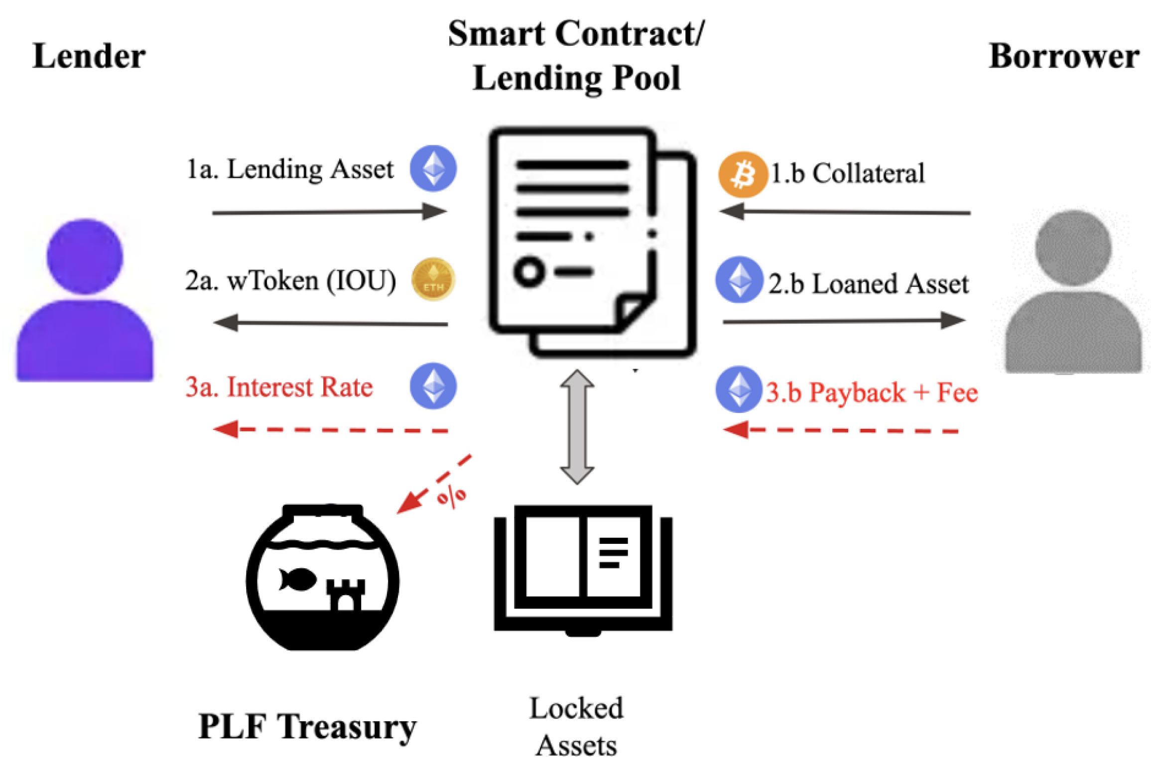
Figure 1 shows a graphic schematic of the process. Starting from the left, Lenders deposit their crypto-assets, such as Ethereum, to earn additional profits. They receive a wrapped token or IOU from the PLF as proof of their deposit. The smart contract acts as a middleman and manages the deposited assets, loans, and liquidations. Borrowers are required to deposit collateral before obtaining a loan. At the end of the loan term, the borrower is obligated to return the borrowed amount plus an interest rate. This interest rate is split pro rata among all lenders, while the remaining interest generated is revenue for the PLF.

Table 1. DeFi Protocols Comparison.

DeFi Protocol	Smart Contract	Investor	User	Financial Service
Protocols for Loanable Funds (PLF)	Lending Pool	Lender	Borrower	Loan
Decentralized Exchange (DEX)	Liquidity Pool	Liquidity Provider	Buyer/Trader	Exchange
Yield Aggregators	Vault	Vault User	-	Asset Management

presents a comparison between DLF and other DeFi protocols such as Decentralized Exchanges and and Yield Aggregators.

1.6. From Over-Collateralization to Risk Appraisal

The current initiatives involve liquidity pools and related DeFi implementations, where any tokenized asset (i.e., insurances, factoring, lending, guaranties of service, and more) is backed by collateral in the search of collateralizing the risk, by means of any of the new digital assets or virtual currencies [25]. Their drawback lies in the over-collateralization, and the volatility caused by new forms of inter-dependency at an unprecedented level is a systemic risk in the future internet of value.

In our opinion, the over-collateralization does not fit properly with invoices risk management, as they are assets with value already appraised in a currency and their risk is related to their liquidity. The euros that will be paid through an invoice are a sort of a stable coin—invoice-euro, for example—so the conversion invoice-euro is pegged to the euro at a discount; say 0.5, 1, or 2 percent or more according to the mora or invoice non-payment rates. It is not a monetary risk, nor a crazy market valuation, but pure risk management that is well known in financial markets which use sophisticated tools.

Unlike the solutions of liquidity pools in the state of the art that use crowd source and oracle approaches to rate risk, we look for alternative formulas that appraise the risk in a fully automated way.

In this reality, there is room to study partly collateralized invoices novel mechanisms using risk management tools that are worthy of exploration and creation in a decentralized implementation that should avoid over-collateralization. These techniques, including the Black–Scholes or the Kelly Criterion [30], are currently studied for their implementation in risk appraisal and management. The work proposed here is interested in the Kelly Criterion for calculating the optimal diversification of investments for creating a portfolio, given a volume of money available for investment, and given some known risk, as it forecasts the optimal benefit achievable.

In the case of decentralized markets with liquidity pools for invoices, provided that we know the volume of money in advance, because it is the liquidity pool’s amount of money, we chose to reformulate the Kelly Criterion so that one might decide whether a given invoice that is partly collateralized can be accepted to be fully collateralized by the liquidity pool, and at what benefit to collect from to compensate the risk. This benefit will be the premium required as a fee for every invoice accepted in the liquidity pool. As this is a new usage of the Kelly Criterion, we named it the Reverse Kelly Criterion as a new formula that calculates the premium to be granted given an invoice with some collateral, as we will see in the following section containing all the details. So this is the goal of our paper: to invent a resilient PLF mechanism that does not require over-collateralization. Let us see how we can do it.

2. Reverse Kelly AMM (rkAMM) Design

Electronic markets use algorithms that decide the price and the amount of liquidity supplied in markets. However, this automation is not complete, as algorithms are managed by humans who intervene to improve their design, or turn them off entirely if conditions become unfavorable, leading to liquidity withdrawals that can exacerbate market volatility. Instead, an Automated Market Maker (AMM) is a type of market that employs a single algorithm to facilitate trades. It is a straightforward, fixed, and predictable approach [31]. AMMs use a constant product rule to swap assets: the product of the reserves of the two assets must remain the same before and after any currency exchange or swap occurs. This concept of holding the value of a function, such as the product of asset reserves during exchanges, evolved into the concept of constant function market making. The fundamental design of constant function market makers was established in [32]. Then, a simple formula, $x·y=k$, set prices and quantities for thousands of different assets using few hundreds lines of code. The AMM today [31] executes upwards of USD 50bn per month in digital assets. The most popular AMM, Uniswap, uses a year of data acquired directly from the public Ethereum blockchain containing over 39 million transactions.

In an AMM, anyone can become a Liquidity Provider (LP) by transferring their digital assets to pools. Fund liquidity can be increased, thus increasing the pool size or creating new ones. In exchange, they receive revenue from a fixed fee on trades (called swaps) by those who demand liquidity from the AMM. Fee revenue is shared equally among LPs in proportion to their investment—so LP returns vary based on the amount of liquidity in a pool (or the pool’s volume or size). LPs can only add or remove liquidity, and prices are set by the AMM algorithm, unlike traditional market makers that can also vary in terms of prices [31].

An algorithm has been conceived following the main guidelines of an AMM for the full collateralization of invoices. As previously stated, AMM were designed to trade two assets by their balance x and y in a liquidity pool to keep up a constant k, as $x·y=k$, so that incoming x means withdrawing y to keep the $x·y$ constant at k. There are several variants of the same scheme [33] to add resilience and utility to the AMM implementation, which must follow their axioms.

In our implementation, we also have liquidity providers that contribute and withdraw their funds at a fee, so that the liquidity pool has some volume V to grant the remaining collateral demanded by the invoices to become fully funded, and premium is required in exchange to compensate the risk aiming at some benefit. From this point of view, it works as a standard community fund for securing risk of participants, but with liquidity providers instead and securing particular assets, such as invoices, that are backed by some collateral. Thus, collateral $c_1$ is added to the pool along with the premium p and, in exchange, the remaining collateral $c_2$ exits, $V·p=k\left(V\right)$, meaning that the constant k is recalculated by the Kelly criterion. Thus, k changes with the new liquidity volume V, and thus with the premium collected.

As briefly introduced, we use the Kelly criterion to calculate the premium contribution to the liquidity pool for missing collateral for a 100% backing invoice, after acknowledging that it is partially backed by some collateral. It is named rkAMM: Reverse Kelly AMM. Performance curves for the rkAMM have been simulated with streams of hundreds of invoices and subsequently analyzed. In its implementation, we have considered the minting of NFTs with the inclusion of terms such as “backing %” of the invoices, risk, and elaboration, which are useful for applying the Kelly Criterion investment formula, among other considerations.

We assumed that for an invoice of amount X, the collateral q is a percentage of X, and the remaining non-collateralized amount is $p=1-q$. We will show how these assumptions have been worked out in the rkAMM.

The Kelly criterion, sometimes referred to as the Kelly strategy or Kelly bet, is a mathematical formula that determines the optimal size for a bet when the expected returns are known. It involves maximizing the expected value of the logarithm of wealth or expected geometric growth rate, as described in [30]. Due to its ability to produce higher wealth compared to any other strategy in the long run (when the number of bets can be infinite), the criterion is also known as the scientific gambling method. The formula has been practically demonstrated in gambling and used to explain diversification in investment management. Rediscovered for its usage in multiple portfolios [34], in the case of digital assets, it was proposed to be used today for risk assessment of derivative products [35]. Here, we saw the opportunity to use the Kelly criterion for “assessing” the liquidity pools for invoice funding.

We use the Kelly criterion to calculate how much premium should be required to contribute to a liquidity pool of size V for an invoice amount of X with a collateral of p, thus demanding the remaining $q=1-p$ collateral out of the rkAMM, as depicted in Figure 2.

We plan to use the rkAMM connected to Byppay [36] because byppay is a system that curates invoices in the sense that groups of three companies acknowledge each other’s rights (invoices) and swap the rights among players to compensate said invoices. Whenever a Byppay among three companies A, B, and C is created, where C invoiced B and B invoiced A so that the chain of payments happened to be from A to B and B to C, schematically A > B > C. In a byppay A > C, that means that A pays directly to C and compensates the A > B and B > C payments. The Proof of Existence (PoE) of the invoices involved in the Byppay considers the mutual knowledge among A and C through B, the common acquaintance of A and C. This PoE and A rating must be sufficient for most of the Byppay cases that require no early payments. This Byppay flow is shown in Figure 3.

If the Byppay is open to third parties other than A, B, and C, then some collateral might be required to B to enhance the PoE and stake of the AB invoice, and the collateralization flow might let the door open to third parties that trust B, or trust A, or trust both, to add collateral to that invoice, privately or openly as a marketplace.

Everyone contributing with collateral will receive some fees; say, a 2% fee out of his piece of contribution to the collateral of the invoices being byppaid. Invoices will be paid some time later, usually in one to three months on average; therefore, the contributed collateral pays off an annual percentage yield (APY) average of 8% to 24%. Contributors of collateral will have advance knowledge of the due date of the invoices to calculate their benefits. Additionally, the greater the connection and knowledge of A and B, the more oracles they would need to rate/score companies, which might fit well on this stage of the byppay flow.

The byppayable invoices with strong collateralization (say, from 50% collateral) are eligible for the rkAMM, and the C will secure the remaining collateral by means of premium to be contributed to said liquidity pool, and then C will receive the full AB amount in advance, while the full amount of the AB invoice will be paid by A to the liquidity pool on the due date.

Whenever A pays, all collateral from the marketplace is returned to the liquidity providers with an additional 2%, and the rkAMM liquidity pool retrieves the collateral provided again with an additional 2%, while B obtains the collateral he might have contributed at the 2% extra, deductible from the fees and bonuses that could have released for the entire Byppay process.

2.1. rkAMM Definition

As introduced, a model inspired by an AMM is proposed to automatically comply with invoice compensation. It is an underlying protocol to conduct exchanges in a decentralized manner through an autonomous trading mechanism. This allows users to exchange their assets without involving centralized financial authorities. Kelly’s formula risk assessment criteria will be used.

The following two assets will be considered:

• The reserve for collateral allocated in the AMM as a liquidity pool, known as Q.
• The reserve of premium collected in the AMM, known as $Premium$.

The collateral serves as a liquidity asset used to complete the compensation of invoices to pay while, in general terms, the premium serves as a protection mechanism of the AMM against the loss of lent collateral and, hopefully, some benefit. Thus, the premium is considered the amount to be paid based on the risk the AMM assumes when lending collateral.

These assets (Q and $Premium$) are exchanged among agents by interacting with the AMM. Agents withdraw liquidity Q at a premium P to compensate the non-collateralized amount of their invoices. This premium contributed by agents is used to compensate the losses the AMM may experience during its operation. The steady remaining premium will be the benefit attributed to the intrinsic performance of the AMM. Additionally, the liquidity providers are enabled to deposit liquidity into the AMM, which allows them to receive a proportional profit out of the accumulated premium based on their shares on the AMM liquidity pool Q according to proposals of [37]. Different premium withdrawal policies and periods are discussed in later sections.

$$Profi{t}_{Premium}=Collecte{d}_{Premium}-Collatera{l}_{UnpaidInvoices}$$

In case there is no liquidity available to collateralize an invoice, the AMM will cover the collateralization of the invoice with the premium collected. Once invoices are fully paid, the remaining premium as profit is expected to be withdrawn in different percentages and periods that will be decided in this paper after several simulations to seek the best withdrawal policy.

2.2. rkAMM Formula

Let us explain the formula of collateral and premium exchanges. To do this, we start with Kelly’s investment formula (Equation (1)):

$$f={\displaystyle \frac{p}{a}}-{\displaystyle \frac{q}{b}}$$

(1)

The following assumptions are made:

• f is the ratio between the amount of collateral requested and the total volume of the rkAMM. The total volume of the rkAMM is computed as the sum of the available collateral Q and, eventually, the accumulated premium at the time.
• p is the collateralized percentage of an invoice. We chose that p is the probability of the invoice to be paid.
• q is the non-collateralized percentage of an invoice amount. We assumed that q is the probability of the invoice to be unpaid.
• $a=q$ given that q is the lack of collateral of an invoice to be fully collateralized by the rkAMM, we interpreted it as the amount of money that could be lost; that is, a, which is known as the partial loss in Kelly’s investment formula.
• From the above: $p=1-q$
• b in Kelly’s investment formula is defined as the partial win. We interpreted this value as the ratio between potential profit and potential loss.

Simplifying the Equation (1) using the assumptions above:

$$f=\frac{1-q}{q}-\frac{q}{b}$$

(2)

For our purpose, the variable to clear is b, which is the ratio of potential profit and potential loss. Thus, solving b from Equation (2):

$$b=\frac{q^2}{1-q(f+1)}$$

(3)

The good news is that, in an invoice, the ratio f and probabilities p and q are always known.

$$f=\frac{NonCollateralize{d}_{Amount}}{Volum{e}_{rkAMM}}=\frac{q·Invoic{e}_{TotalAmount}}{Volum{e}_{rkAMM}}$$

(4)

The potential loss is known, since it is the amount of collateral that the rkAMM lends to the user, which is equal to the non-collateralized amount. Then, the potential profit is what we have called the $premium$. So far, all the variables are known, except for the $premium$.

The variable to clear is the potential profit, which is the premium, since it is the amount the rkAMM can earn if the user repays the collateral and the invoice in full. That is why it is a potential profit, because the rkAMM is assuming a risk based on an amount, which is compensated by a premium, which will not be repaid but kept for the collateral and liquidity providers who assumed the risk.

So, we can formulate the following equation of b, whose value is known from solving Equation (3):

$$b=\frac{PotentialProfit}{PotentialLoss}=\frac{Premium}{q·Invoic{e}_{TotalAmount}}$$

(5)

Clearing the $premium$ variable:

$$Premium=b·q·Invoic{e}_{TotalAmount}$$

(6)

In summary, we have the following values on Equation (6):

• $premium$: variable to calculate.
• b: calculated from Equation (3) since f and q are known.
• q: known since it is the amount to be collateralized.
• $Invoic{e}_{TotalAmount}$: known as an invoice parameter.

2.3. Illustrative Example

Firs, the rkAMM initial condition is presented in

Table 2. Initial rkAMM situation.

rkAMM Initial Condition	Value
Liquidity available	1800
Premium deposited	0
Volume (Liquidity + Premium)	1800

.

Then, an invoice that has a p collateral and is demanding q over the total amount is applying for the rkAMM service. This scenario is contemplated in

Table 3. Invoice amounts.

Invoice	%	Amount
Collateralized amount (p)	60	1200
Non-collateralized amount (q)	40	800
Total	100	1200

.

Using Equation (4), the value of f is:

$$f=\frac{NonCollateralize{d}_{Amount}}{Volum{e}_{rkAMM}}=\frac{800}{1800}=0.444...$$

Since $q·Invoic{e}_{TotalAmount}=NonCollateralize{d}_{Amount}$.

Then, from Equation (3), the value of b is:

$$b=\frac{q^2}{1-q(f+1)}=\frac{0.4^2}{1-0.4(0.444+1)}=0.3789\to 37.89\%$$

Recall that $q·Invoic{e}_{TotalAmount}$ is proportional but essentially different from q because with p, q, and b and a, we are working with probabilities and ratios.

From Equation (5), we have:

$$b={\displaystyle \frac{PotentialProfit}{PotentialLoss}}=\frac{Premium}{q·Invoic{e}_{TotalAmount}}=\frac{Premium}{800}=0.3789$$

Clearing premium from the previous equation as in Equation (6):

$$Premium=800·0.3789=303.16\left(\mathrm{euro}\right)$$

Finally, the rkAMM goes on as follows and the intermediate situation can be seen in

Table 4. Intermediate rkAMM situation after accepting an invoice (collateralization).

rkAMM Intermediate Condition	Value (Euro)
Liquidity available	1000
Premium deposited	303.16
Volume (Liquidity + Premium)	1303.16

.

At this point, collateral is withdrawn from the pool and $premium$ has been deposited. What will happen if the payer does not repay the invoice will be matter of study with several scenarios that will be covered in the next section.

So, following this example, at some point, the user or his client will repay the collateral, which is EUR 800. Finally, the rkAMM situation is shown in

Table 5. Final rkAMM situation after collateral repaid.

rkAMM Final Condition	Value (Euro)
Liquidity available	1800 (1000 + 800)
Premium deposited	303.16
Volume (Liquidity + Premium)	2103.16

:

The rkAMM has made a profit because it has assumed the risk by supporting the non-collateralized amount of the invoice for some time in between the collateral provided by the rkAMM; the collateral is later repaid at the invoice due date, sooner or later.

3. Simulations Setup

A set of simulations have been developed based on five scenarios to study typical situations that may occur. Invoices used in the scenarios have the structure shown in

Table 6. Invoice attributes definition.

Value	Description
Id Invoice	Invoice identifier
Non-coll. %	Value between 5% and 49%
Non-coll. amount	Value between 100 and 2000 (euro)
Collateralized date	Day when the invoice is collateralized
Collateralized status	True if the invoice is collateralized/False otherwise
Payment delay days	Value between 30 and 120 (days)
Paid status	True if the non-coll. amount is repaid/False otherwise

:

Key attributes such as invoice amounts or the percentages of collateral or nonpayment are modified at each scenario to analyze the behavior of the rkAMM. The complete set of attributes used to simulate the scenarios is shown in

Table 7. Attributes used to simulate default (non-payment) and hack scenarios.

Description	Value	Comment	Fixed or Variable Parameter (across Different Scenarios)
Number of simulations	100	Number of simulations to determine the common behavior of the rkAMM	Fix
Initial collateral $Q_0$	10,000 (euro)	This amount is the initial liquidity in the LP.	Fix
Initial premium	0	N/A	Fix
Number of invoices	500	Max. value of invoices to process	Fix
Range of % from invoices to collateralize	5–49%	Max. and min. values allowed for invoice collateralization	Variable only for scenario 5 and Hack scenarios
Range of amount from invoices to collateralize	100–2000 (euro)	Max. and min. amounts allowed to be collateralized. As the initial collateral $Q_0$ is fixed to 10,000, we set the simulations in the range 0.1–20% of the initial liquidity	Variable only for scenario 4
Invoice payment period range	30–120 (days)	Max. and min. delays in days for the payment of invoices	Variable only for scenario 3
Range of liquidity contribution by LPs	0–0	Max. and min. amounts of liquidity contribution to the rkAMM	Variable only for scenario 1
Non-payment probability	0%	The probability that collateral on an invoice will never be paid back	Variable only for scenario 2 and Hack scenarios
Hack probability	0%	The probability of including false invoices that will never be paid may affect the performance of the rkAMM	Variable only for Hack scenarios
Probability of contribution by LPs	0%	The probability that an LP makes a liquidity deposit to the rkAMM	Variable only for scenario 1
Maximum days	500	Days on which invoice entries are allowed	Fix to the number of invoices
Additional days	30	Extra days for simulations to reach the steady state of the rkAMM	Fix
Number of days of the simulation	650	Total days of simulation. Max. days + Max. delay invoice payment + Additional days	Fix to maximum (days + delays) + additional days

.

In this research, neither predictive nor classification models are used, since the rkAMM does not need to predict future behavior of invoice sets and does not need to classify them. Simulations only intend to study the final outcome of the rkAMM based on sets of invoices generated randomly through uniform distribution.

At every scenario, many sets (from 100 sets) of invoices are generated to obtain solid statistical ground.

3.1. Scenarios

The five scenarios for the simulations are:

Scenario 1—Here, we experiment with the growing contribution of collateral by liquidity providers (LP) on a growing rate of the volume of collateral (Q) in the rkAMM, in the pool. As the Probability of Contribution is fixed at 50% every day, the Range of Liquidity contribution is being experimented in three conditions: 1% of initial Q at every contribution for scenario 1.1 (Very Low), 5% of initial Q for case 1.2 (Low), 10% of initial Q for case 1.3 (Medium), and 25% of initial Q for case 1.4 (Max).

Scenario 2—Here, we experiment with sets of non-payments back to the rkAMM. The attribute changed in this scenario is the non-payment probability, in three cases: 2% of invoices for case 2.1 (Low), 5% for case 2.2 (Medium), and 20% for case 2.3 (Max).

Scenario 3—Here, we experiment with Increasing Delay in invoice payments. The payment period ranges from what is considered short to long. Payment period ranges are: 30–60 days for case 3.1 (Short), 60–90 days for case 3.2 (Medium), and 90–120 days for case 3.3 (Long).

Scenario 4—Here, we experiment with the $Amount$ to be collateralized, which will depend on a variable percentage of the initial volume of collateral ($Q_0$) in the rkAMM. The Demanded collateral to the pool is in three cases: 1% of initial $Q_0$ for case 4.1 (Low), 10% of initial $Q_0$ for case 4.2 (Medium), and 25% of initial $Q_0$ for case 4.3 (Max).

Scenario 5—Different % to be collateralized. This is slightly different from scenario 4, as here, we work with the percentage only and not with the amount to be collateralized. Although they are, of course, directly related, the sensitivity of the pool to the amount of collateral comes out with different outputs. The range of % collateral p of invoices is set to three cases. Range of % collateral p: 55% for case 5.1 (Low), 75% for case 5.2 (Medium), and 90% for case 5.3 (Max).

In addition to the scenarios proposed above, there is an additional set consisting of those situations in which there are malicious actors trying to take advantage of the rkAMM operation. These scenarios foresee a hack of the rkAMM; that is, there is a high number of false, bogus invoices. A false invoice is considered one for which the collateral given away by the rkAMM will never be paid back. The purpose of this hack from the attacker’s point of view is to drain the rkAMM liquidity.

Hack scenario—To hack the rkAMM, the following attributes from the default scenario are modified to produce a set of hacking cases:

• Range of % from invoices to collateralize: 49% (Max), 30% (Medium), and 10% (Low)
• Non-payment probability: 10% (Low), 50% (Medium), and 100% (Max) crossed with all the ranges of % from invoices to collateralize.

3.2. Technical Description of the Simulator

The simulator has been developed in Python. For the analysis and presentation of the experiment metrics, common analysis and data visualization libraries have been used.

The invoices have been structured in a list of dictionaries to execute the simulations. Each invoice is defined by a dictionary of seven keys and values, and this dictionary in turn occupies a position in a list of invoices.

Regarding the functions of the simulation, those that allow modification of the volumes of liquidity, collateral, and premium have been defined. In addition, a function has been developed to calculate the premium based on the requested collateral, as explained in Section 2.2 of this document.

To implement the simulation, there is a main function that randomly generates a set of invoices based on the previously defined parameters in Table 6. The flow of invoices is steady at one invoice per day of any random amount and collateral within the range of parameters described for the simulations in Table 7. When they are accepted in the liquidity pool, then premium is contributed, and collateral is withdrawn on the same day. Otherwise, when they are not accepted, they are simply discarded, and the next day comes for the next invoice.

The simulation also performs daily synchronization of the liquidity contributions of random amounts in the range established by the parameters. The invoices that are repaid achieve this with a random day within a minimum number of days (often 30 days are chosen) and a maximum of 120 days. On the other hand, invoices that are not repaid are programmed for a delay large enough for a due date well after the simulation, with a maximum delay of 100,000, since Python 3 int does not have a maximum size and using math.inf may impact the efficiency of our code.

Then, the number of days for each simulation is the number of the stream of invoices (one invoice per day), plus the maximum delay of 120 days and an additional number of few extra days. For instance, for a stream of 500 invoices, a maximum delay of 120 days, and 30 extra days, the limit is $500+120+30=650$ days per simulation.

Every scenario is defined by the parameters mentioned in Table 7. A batch of 100 simulations per scenario are run; thus, the metrics are calculated as an average per batch.

To simulate several scenarios of unpaid invoices, a random number of invoices will be chosen not to be repaid, so that they pay the premium to be accepted in the rkAMM and obtain collateral that is, however, never returned to the rkAMM. The rkAMM will try to compensate the losses by means of the premium, and we will see how resilient it is at the end of the run of all simulations.

The rkAMM also contemplates the possibility of withdrawing the premium collected: the withdrawal period and the premium percentage to be withdrawn can be set up.

Last, but not least, the hack of the system, consisting of extenuating the rkAMM by a flow of bogus invoices, is intentionally left unpaid. This is achieved by increasing the hack probability that is directly proportional to the non-payment probability of invoices.

3.3. Repository of the rkAMM

There is a GitHub repository (https://github.com/ballesterosbr/rkAMM, last access on 7 February 2023) of the rkAMM for running and testing the simulations.

4. Results

Several batches of simulations of the behavior of the rkAMM based on the scenarios defined in Section 3.1 of this document were performed. Each batch is a case in a scenario, and performances will be analyzed. The plots of the liquidity and the premium will be presented for the most relevant scenarios.

4.1. Limitations

As stated, in the event that the rkAMM does not have liquidity nor premium to collateralize an invoice, this invoice is discarded, a day passes through, and the next invoice will be evaluated. When the rkAMM regains the collateral granted to a former collateralized invoice or the amount to be collateralized for a new invoice is less than the available liquidity in the rkAMM, the invoice might be granted for collateralization.

In the simulations, the profit percentage shows the result of the rkAMM. This benefit will be distributed among those LPs that have deposited liquidity into the rkAMM, so it is expected that this will have an impact on the rkAMM profit.

After inspecting the scenarios, our proposal of the rkAMM implies that the invoice percentage to collateralize is advised to never be greater than 49% or lower than 5%.

4.2. Metrics

A set of metrics is defined to describe the behavior of the rkAMM and analyse the results of the simulations: plots of the volume of the rkAMM, the premium collected, the premium withdrawn, and the resulting liquidity as an addition of the volume and the remaining premium. To better understand the metrics,

Table 8. Baseline scenario output. Scenario 5 and 30 days of withdrawal period.

Value	No Premium Withdrawn	Premium Withdrawn	Premium vs. No Premium Withdrawn	Description
Number of simulations	100.0	100.0	0.0%	Number of simulations conducted.
Simulation time period (days)	650.0	650.0	0.0%	Total number of days on which the simulation has been conducted.
Total of invoices	500.0	500.0	0.0%	Number of invoices to be processed by the rkAMM.
Average of accepted invoices (collateralized)	350.96	179.34	−48.9%	Number of invoices accepted by the rkAMM.
% of accepted invoices (collateralized)	70.19	35.87	−48.9%	% of invoices accepted by the rkAMM.
Average of paid invoices (capital returned)	350.96	179.34	−48.9%	Number of accepted invoices for which collateral has been returned.
% of paid invoices (capital returned)	100.0	100.0	0.0%	% of accepted invoices for which collateral has been returned.
Average of unpaid invoices (capital not returned)	0.0	0.0	0.0%	Number of accepted invoices for which the collateral has not been returned.
% of unpaid invoices (capital not returned)	0.0	0.0	0.0%	% of accepted invoices for which the collateral has not been returned.
Average loss due to unpaid invoices)	0.0	0.0	0.0%	Amount (in EUR) lost due to unpaid invoices.
Total collateral covered	329,583.29	124,772.17	−62.14%	Total amount of collateral borrowed by the rkAMM.
Total collateral covered x (i.c.)	32.96	12.48	−62.14%	Total amount of collateral borrowed by the rkAMM with respect to the initial collateral $Q_0$.
Total premium withdrawn	0.0	33,161.86	100.0%	Total premium withdrawn.
Total premium withdrawn x (i.c.)	0.0	3.32	100.0%	Total premium withdrawn with respect to the initial collateral $Q_0$.
Remaining rkAMM premium	10,344.89	0.0	−100.0%	Remaining premium in the rkAMM after the simulation ends.
Remaining rkAMM premium x (i.c.)	1.03	0.0	−100.0%	Remaining premium in the rkAMM after the simulation ends with respect to the initial collateral $Q_0$.
Final rkAMM volume	98,416.65	29,049.41	−70.48%	Total volume of the rkAMM after simulation.
rkAMM profit	88,416.65	52,211.27	−40.95%	rkAMM profit without including initial collateral $Q_0$.
rkAMM profit percentage	884.17	522.11	−40.95%	rkAMM profit percentage without including initial collateral $Q_0$.

shows an example. At the end of a batch of 100 simulations of the three cases of scenario 5, we have the averaged measures.

The set of

Table 9. rkAMM results. Every day, 50% of the premium obtained is withdrawn.

Scenario	% Accepted Invoices		% Unpaid Invoices		Avg. Loss due to		Total Collateral Covered		Total Premium with.		Remaining Premium		rkAMM Profit
#	(Collateralized)		(Capital Not Returned)		Unpaid Invoices		x (i.c.)		x (i.c.)		x (i.c.)		Percentage
	No With.	With.	No With.	With.	No With.	With.	No With.	With.	No With.	With.	No With.	With.	No With.	With.
1.1	69.39	36.29	0.0	0.0	0.0	0.0	32.45	12.62	0.0	3.43	1.01	0.0	872.63	537.8
1.2	87.42	69.22	0.0	0.0	0.0	0.0	43.69	31.48	0.0	7.03	4.02	0.0	1601.63	1556.73
1.3	93.55	86.47	0.0	0.0	0.0	0.0	47.95	43.29	0.0	7.91	5.46	0.0	2407.74	2437.59
1.4	99.18	97.5	0.0	0.0	0.0	0.0	52.04	50.75	0.0	7.9	6.86	0.0	4901.76	4897.91
2.1	56.1	22.94	1.9	2.02	4512.98	1472.62	24.46	7.0	0.0	1.96	0.28	0.0	554.43	199.11
2.2	51.57	21.56	5.11	4.99	11,049.93	3097.52	21.69	6.37	0.0	1.76	0.19	0.0	447.58	160.02
2.3	36.52	15.0	19.98	19.76	26,130.04	8128.02	13.09	4.07	0.0	1.07	0.05	0.0	117.39	34.6
3.1	80.55	35.11	0.0	0.0	0.0	0.0	39.97	12.42	0.0	3.3	2.81	0.0	748.97	359.58
3.2	52.98	22.82	0.0	0.0	0.0	0.0	23.54	7.36	0.0	1.97	0.29	0.0	561.77	213.34
3.3	32.34	16.04	0.0	0.0	0.0	0.0	13.08	5.27	0.0	1.4	0.02	0.0	340.62	150.89
4.1	100.0	100.0	0.0	0.0	0.0	0.0	5.0	5.0	0.0	0.74	0.73	0.0	72.62	73.62
4.2	48.68	18.1	0.0	0.0	0.0	0.0	24.34	9.05	0.0	4.01	0.31	0.0	578.46	457.26
4.3	21.6	8.21	0.0	0.0	0.0	0.0	27.0	10.27	0.0	5.14	0.22	0.0	728.34	608.29
5.1	96.87	30.29	0.0	0.0	0.0	0.0	50.2	10.16	0.0	8.05	13.61	0.0	2182.86	903.32
5.2	32.56	22.87	0.0	0.0	0.0	0.0	10.79	6.84	0.0	0.72	0.03	0.0	114.05	72.34
5.3	23.46	22.94	0.0	0.0	0.0	0.0	7.12	6.85	0.0	0.08	0.01	0.0	8.49	8.18

i.c. = initial collateral Q₀; No With. = No Premium Withdrawn; With. = Premium Withdrawn.

,

Table 10. rkAMM hack scenario results. Every day, 50% of the premium obtained is withdrawn.

Hack	% Accepted Invoices		% Unpaid Invoices		Avg. Loss due to		Total Collateral Covered		Total Premium with.		Remaining Premium		rkAMM Profit
Prob.	(Collateralized)		(Collateralized)		Unpaid Invoices		x (i.c.)		x (i.c.)		x (i.c.)		Percentage
	No With.	With.	No With.	With.	No With.	With.	No With.	With.	No With.	With.	No With.	With.	No With.	With.
10%	99.94	47.72	9.78	9.91	51,136.77	19,804.32	52.3	20.08	0.0	26.79	16.33	0.0	2300.96	3008.99
	32.63	18.19	10.16	9.93	10,627.94	5147.54	10.52	5.12	0.0	0.89	0.04	0.0	80.26	38.79
	19.16	18.51	9.8	9.54	5211.17	4895.74	5.38	5.21	0.0	0.06	0.01	0.0	−45.71	−42.75
50%	99.95	13.96	50.19	50.13	264,936.55	22,607.54	52.8	4.52	0.0	6.55	1.74	0.0	483.79	572.29
	11.4	6.68	49.93	49.64	14,482.67	9884.92	2.92	1.96	0.0	0.32	0.01	0.0	−94.93	−66.01
	7.39	7.11	49.24	48.86	10,009.92	9823.79	2.01	2.0	0.0	0.02	0.0	0.0	−97.73	−95.88
100%	98.99	2.35	100.0	100.0	515,511.86	10,923.77	51.55	1.09	0.0	0.84	0.33	0.0	−66.94	−16.02
	2.75	2.15	100.0	100.0	11,719.05	9992.76	1.17	1.0	0.0	0.15	0.01	0.0	−99.44	−84.9
	2.27	2.24	100.0	100.0	10,077.26	9962.26	1.01	1.0	0.0	0.01	0.0	0.0	−99.61	−98.48

i.c. = initial collateral Q₀; No With. = No Premium Withdrawn; With. = Premium Withdrawn. Colored values refer to those cases in which the rkAMM profit percentage is negative.

,

Table 11. rkAMM results. Every 30 days, 50% of the premium obtained is withdrawn.

Scenario	% Accepted Invoices		% Unpaid Invoices		Avg. Loss due to		Total Collateral Covered		Total Premium with.		Remaining Premium		rkAMM Profit
#	(Collateralized)		(Capital Not Returned)		Unpaid Invoices		x (i.c.)		x (i.c.)		x (i.c.)		Percentage
	No With.	With.	No With.	With.	No With.	With.	No With.	With.	No With.	With.	No With.	With.	No With.	With.
1.1	69.64	66.23	0.0	0.0	0.0	0.0	32.5	30.24	0.0	1.5	0.96	0.01	868.36	860.4
1.2	87.49	86.28	0.0	0.0	0.0	0.0	43.73	42.93	0.0	4.32	4.05	0.02	1610.66	1603.16
1.3	93.97	93.16	0.0	0.0	0.0	0.0	48.18	47.8	0.0	5.78	5.48	0.02	2432.65	2428.88
1.4	99.11	98.9	0.0	0.0	0.0	0.0	51.8	51.71	0.0	7.02	6.83	0.02	4868.1	4828.38
2.1	56.42	50.38	2.16	2.06	5418.73	4547.89	24.66	21.2	0.0	0.7	0.25	0.0	561.84	501.42
2.2	51.99	48.28	5.15	4.88	11,524.67	9398.72	21.9	19.79	0.0	0.64	0.18	0.0	453.12	424.97
2.3	37.41	32.0	19.79	19.9	27,238.25	21,592.14	13.65	10.88	0.0	0.36	0.06	0.0	131.24	97.31
3.1	80.74	78.38	0.0	0.0	0.0	0.0	40.1	38.35	0.0	3.04	2.89	0.02	757.77	759.62
3.2	52.49	49.01	0.0	0.0	0.0	0.0	23.35	21.08	0.0	0.75	0.31	0.01	561.81	529.75
3.3	32.82	29.5	0.0	0.0	0.0	0.0	13.22	11.76	0.0	0.35	0.03	0.0	344.3	312.77
4.1	100.0	100.0	0.0	0.0	0.0	0.0	5.0	5.0	0.0	0.74	0.73	0.0	72.53	73.77
4.2	48.95	41.87	0.0	0.0	0.0	0.0	24.48	20.93	0.0	0.81	0.3	0.0	581.6	525.56
4.3	21.88	15.94	0.0	0.0	0.0	0.0	27.34	19.93	0.0	1.39	0.21	0.01	728.41	584.32
5.1	96.83	95.82	0.0	0.0	0.0	0.0	49.92	49.22	0.0	13.94	13.49	0.06	2172.02	2216.21
5.2	32.11	30.23	0.0	0.0	0.0	0.0	10.77	9.81	0.0	0.23	0.03	0.0	113.91	103.73
5.3	23.7	23.16	0.0	0.0	0.0	0.0	7.14	6.92	0.0	0.05	0.01	0.0	8.52	8.26

i.c. = initial collateral Q₀; No With. = No Premium Withdrawn; With. = Premium Withdrawn.

,

Table 12. rkAMM hack scenario results. Every 30 days, 50% of the premium obtained is withdrawn.

Hack	% Accepted Invoices		% Unpaid Invoices		Avg. Loss due to		Total Collateral Covered		Total Premium with.		Remaining Premium		rkAMM Profit
Prob.	(Collateralized)		(Collateralized)		Unpaid Invoices		x (i.c.)		x (i.c.)		x (i.c.)		Percentage
	No With.	With.	No With.	With.	No With.	With.	No With.	With.	No With.	With.	No With.	With.	No With.	With.
10%	99.96	99.64	9.86	9.77	51256.79	50,736.8	52.45	52.32	0.0	17.67	16.46	0.07	2309.78	2442.9
	32.12	29.94	10.14	9.83	10,675.98	9172.03	10.39	9.48	0.0	0.29	0.04	0.0	77.82	76.84
	18.65	18.08	10.07	10.52	5323.51	5332.92	5.2	5.05	0.0	0.04	0.01	0.0	−47.04	−47.31
50%	99.95	99.43	50.21	50.05	264,606.12	261,539.02	52.69	52.11	0.0	6.09	1.84	0.02	483.06	904.98
	11.31	9.8	49.37	50.69	14,483.85	13,215.62	2.93	2.66	0.0	0.11	0.01	0.0	−94.73	−86.87
	7.07	7.08	50.85	49.38	10,046.43	9880.93	2.0	1.96	0.0	0.02	0.0	0.0	−98.11	−96.5
100%	99.0	93.26	100.0	100.0	514,687.26	472,315.05	51.47	47.23	0.0	3.21	0.35	0.01	−64.97	222.34
	2.68	2.6	100.0	100.0	11,725.34	11,529.51	1.17	1.15	0.0	0.02	0.01	0.0	−99.42	−97.86
	2.23	2.21	100.0	100.0	10,074.25	10,036.04	1.01	1.0	0.0	0.01	0.0	0.0	−99.58	−99.2

i.c. = initial collateral Q₀; No With. = No Premium Withdrawn; With. = Premium Withdrawn. Colored values refer to those cases in which the rkAMM profit percentage is negative.

,

Table 13. rkAMM results. Every 90 days, 50% of the premium obtained is withdrawn.

Scenario	% Accepted Invoices		% Unpaid Invoices		Avg. Loss due to		Total Collateral Covered		Total Premium with.		Remaining Premium		rkAMM Profit
#	(Collateralized)		(Capital Not Returned)		Unpaid Invoices		x (i.c.)		x (i.c.)		x (i.c.)		Percentage
	No With.	With.	No With.	With.	No With.	With.	No With.	With.	No With.	With.	No With.	With.	No With.	With.
1.1	69.96	70.01	0.0	0.0	0.0	0.0	32.73	32.71	0.0	1.04	1.1	0.18	881.2	889.71
1.2	86.84	86.55	0.0	0.0	0.0	0.0	43.56	43.39	0.0	3.56	3.93	0.45	1591.24	1607.24
1.3	93.64	94.02	0.0	0.0	0.0	0.0	48.16	48.19	0.0	5.16	5.47	0.5	2409.92	2435.5
1.4	99.21	99.22	0.0	0.0	0.0	0.0	51.9	51.77	0.0	6.32	6.83	0.51	4844.95	4838.42
2.1	56.46	52.61	1.95	1.95	4693.43	4125.03	24.79	22.42	0.0	0.34	0.31	0.04	571.75	523.22
2.2	51.15	51.48	5.08	4.88	10,905.05	10,265.56	21.45	21.71	0.0	0.3	0.17	0.04	436.98	451.74
2.3	34.42	34.65	20.42	20.04	24,583.38	24,005.7	12.07	12.05	0.0	0.14	0.05	0.01	102.84	100.99
3.1	81.62	80.54	0.0	0.0	0.0	0.0	40.82	39.86	0.0	2.65	3.01	0.38	766.99	768.17
3.2	52.74	50.55	0.0	0.0	0.0	0.0	23.44	22.15	0.0	0.39	0.33	0.07	566.55	543.55
3.3	32.17	31.62	0.0	0.0	0.0	0.0	12.71	12.48	0.0	0.13	0.03	0.01	332.73	323.79
4.1	100.0	100.0	0.0	0.0	0.0	0.0	5.0	5.0	0.0	0.69	0.73	0.05	72.64	73.59
4.2	49.71	46.7	0.0	0.0	0.0	0.0	24.86	23.35	0.0	0.41	0.31	0.06	590.31	560.45
4.3	22.91	20.52	0.0	0.0	0.0	0.0	28.64	25.65	0.0	0.63	0.21	0.06	762.75	700.41
5.1	96.81	96.73	0.0	0.0	0.0	0.0	50.16	50.17	0.0	12.5	13.51	1.24	2177.66	2199.24
5.2	32.29	31.89	0.0	0.0	0.0	0.0	10.79	10.58	0.0	0.09	0.03	0.01	113.95	112.06
5.3	23.82	23.33	0.0	0.0	0.0	0.0	7.16	7.1	0.0	0.02	0.01	0.0	8.54	8.48

i.c. = initial collateral Q₀; No With. = No Premium Withdrawn; With. = Premium Withdrawn.

and

Table 14. rkAMM hack scenario results. Every 90 days, 50% of the premium obtained is withdrawn.

Hack	% Accepted Invoices		% Unpaid invoices		Avg. Loss due to		Total Collateral Covered		Total Premium with.		Remaining Premium		rkAMM Profit
Prob.	(Collateralized)		(Collateralized)		Unpaid Invoices		x (i.c.)		x (i.c.)		x (i.c.)		Percentage
	No With.	With.	No With.	With.	No With.	With.	No With.	With.	No With.	With.	No With.	With.	No With.	With.
10%	99.96	99.95	10.08	9.87	52,195.52	51,985.91	52.44	52.4	0.0	15.42	16.39	1.34	2301.21	2337.35
	33.05	32.1	10.08	10.04	10,762.52	10,505.58	10.83	10.45	0.0	0.12	0.04	0.01	85.23	80.5
	19.02	18.4	10.0	10.07	5192.23	5353.66	5.29	5.16	0.0	0.02	0.01	0.0	−45.62	−47.39
50%	99.89	99.91	50.12	49.94	262,371.99	260,757.48	52.29	52.35	0.0	3.25	1.79	0.25	483.09	659.2
	11.59	10.17	49.47	50.4	14,717.05	13,754.29	3.06	2.69	0.0	0.05	0.01	0.0	-94.57	−91.64
	7.21	7.23	50.1	49.61	10,057.43	9962.06	2.02	2.02	0.0	0.01	0.0	0.0	−98.19	−97.24
100%	99.08	97.19	100.0	100.0	518,522.18	501,747.51	51.85	50.17	0.0	1.18	0.39	0.09	−60.73	26.59
	2.71	2.66	100.0	100.0	11,712.08	11,620.56	1.17	1.16	0.0	0.01	0.01	0.0	−99.38	−98.56
	2.23	2.19	100.0	100.0	10,076.63	10,054.62	1.01	1.01	0.0	0.01	0.0	0.0	−99.61	−99.39

i.c. = initial collateral Q₀; No With. = No Premium Withdrawn; With. = Premium Withdrawn. Colored values refer to those cases in which the rkAMM profit percentage is negative.

show results for all scenarios, which will be discussed in the next section. The result plots are also presented for a better understanding of the results. To avoid overloading this section and to facilitate reading, only the plots from scenario 5 with a Premium withdrawal period of 30 days are presented, since it is considered the most relevant and frequent scenario to occur in the rkAMM deployment. The plots for the other scenarios are summarized in the Appendix A section. The results on mean average over a 100 runs batch per every case and scenario are less than 0.7% standard error on the rkAMM profit measure. We think this is reasonably sound for backing the conclusions over the discussion of the results.

In addition to the scenarios results of the tables presented above and the curves from scenario 5 shown in Figure 4, in the following Figure 5 and Figure 6, there is a comparative analysis of the rkAMM profit of all the scenarios. Figure 5 shows a comparison between the rkAMM profit when there is no premium withdrawal, and when there is premium withdrawn but, depending on the frequency, the premium is withdrawn. Figure 6 shows the rkAMM percentage of profit difference between scenarios in which the premium is withdrawn and where it is not. Premium withdrawal intervals are 1, 30 and 90 days.

One can see that the rkAMM profit is not affected by the premium withdrawal in the majority of the scenarios. It can even be concluded that the frequency with which the premium is withdrawn does not have a significant impact either, except for the scenarios in which the premium is withdrawn every day.

Surprisingly, only the daily premium withdrawal causes the rkAMM profit to be only a few points lower than the rkAMM profit when there is no premium withdrawal, while in the other scenarios with lower frequency (of +30 days), even the performance is boosted in some cases.

Figure 7 shows the overall profit of rkAMM taking into account all possible scenarios and premium withdrawal periods.

As in the other scenarios, besides the hack scenarios tables, Figure 8 illustrates the curves of that simulation. Figure 9 shows that practically one-third of the scenarios is affected to a greater extent by the premium withdrawal, and therefore the rkAMM profit is altered. Further, this impact turns out to be positive and the performance of the AMM for this set of scenarios is better when premium is withdrawn periodically, especially with invoices collateralized at 51%. The best cases are those in which the invoices are collateralized at 51%, although the rkAMM profit decreases as the hack probability increases.

As for the percentage difference with respect to withdrawing premium or not shown in Figure 10, the scenarios in which premium is withdrawn every 30 days with 51% collateralized invoices present an improvement of 5%, 89% and 249% with hacking probabilities of 10%, 50%, and 100%, respectively. Regarding daily withdrawals, the only favorable case is found when invoices are collateralized at 51% with a hacking probability of 10%. Finally, for premium withdrawals every 90 days, the most remarkable case is that in which invoices are collateralized at 51%, with a hack probability of 50%. The rest of the scenarios have presented a worse performance when there is a periodic premium withdrawal.

All of the above is summarized in Figure 11 where it can be seen the overall profit of rkAMM taking into account all possible scenarios and premium withdrawal periods.

5. Withdrawn Premium Analysis

In this section, a detailed analysis of the results of the previous section is carried out.

First, it must be taken into account that the rkAMM also grants collateral of invoices from the premium if it does not have sufficient liquidity. This happens for all scenarios and positively affects both the final premium values and the total volume of the rkAMM.

Considering the results, the more adverse the scenario, the lower the premium withdrawn from the rkAMM will be. The same happens with the remaining premium in the rkAMM: the worse the scenario, the lower the amount available. This is because the rkAMM will try to collateralize with the premium due to lack of liquidity, which is expected behavior in adverse scenarios. However, this general rule has some exceptions.

Scenario 1: The greater the increase in liquidity shows nearly a 100% match of the results when no premium is withdrawn.

As liquidity increases, the difference rises from an approximate −50% to a −1% difference on accepted/paid invoices increases. In all cases, all collateralized invoices are paid.

When there is a greater liquidity contribution, the total covered is increased. However, in the worst case of liquidity contribution (scenario 1.1), there is a 60% difference in terms of the total collateral covered. This difference is drastically reduced in the 1.4 case, where it is only 1%.

Concerning the premium managed by the rkAMM in these cases, it is increasing as more liquidity is provided, which was to be expected, given that a larger number of invoices are collateralized.

Regarding the benefit of the rkAMM, the greater the contribution of liquidity, the greater the profit rkAMM. However, the withdrawal of premium does not affect the benefit of the premium by itself, since there are scenarios in which premium is withdrawn and a larger benefit is obtained (even if only 1%) than those in which there is no withdrawal of premium. This is because in cases where there is no premium withdrawal, less premium is collected than in the cases where premium is withdrawn.

Scenario 2: Facing an increase in unpaid invoices, the scenarios with premium withdrawal and those without have the same shape, although the absolute values are affected and the results are worse in the cases of the highest numbers of unpaid invoices.

The number of collateralized invoices decreases. The same happens for the amount of collateral covered and the rkAMM profit.

Regarding the losses resulting from unpaid invoices, the relationship between scenarios is maintained despite the increase in the number of these invoices.

Scenario 3: The larger the delay in the payment of the invoices, the lower the premium that can be withdrawn and the lower the remaining premium in the case where the premium is not withdrawn. The shorter the payment term, the better the liquidity of the rkAMM.

The number of collateralized invoices will be lower, but the relationship between the scenarios with premium withdrawal and those without is variable, and it worsens in the scenarios where there are greater delays in the invoice payments. The same happens for the amount of collateral covered.

The rkAMM profit is lower, along with a growing delay in the payment of invoices.

Scenario 4: The greater the amount to be collateralized, the better the results of the rkAMM are in terms of its performance, since more liquidity is collateralized. Therefore, a higher premium is obtained and the larger the benefit of the rkAMM. In summary, better results are achieved the higher the risk assumed by rkAMM.

The number of collateralized invoices decreases, but the relationship between the scenarios with premium withdrawal and those without is variable, and it worsens in scenarios in which there are increasingly large invoices (of larger amounts). Despite the fact that the collateral is covered and the rkAMM profit increases, the two scenarios have the same behavior.

Scenario 5: Same pattern as scenario 4. The higher the percentage to be collateralized, the worse the results of the rkAMM. It can also be determined that the higher the percentage of collateralization of the invoices, the more similar the results between scenarios where premium is withdrawn and where it is not.

The number of collateralized invoices decreases; however, the relationship between the scenarios in which premium is withdrawn and those in which it is not decreases until it is almost equal to the scenario in which the invoices are almost completely collateralized. The same happens for the amount of collateral covered and profit rkAMM as the amount to be collateralized increases.

Hack Scenario: The larger the hack probability and the amount to collateralise, the worse the results of the AMM in terms of its performance. However, in some cases, premium withdrawal performs better in terms of AMM profit for withdrawal periods of 30 and 90 days.

Losses due to unpaid invoices, as expected, increase as the probability of hacking increases. On the contrary, the amount of collateral covered decreases as the probability of hacking and the amount to be collateralized increases. The same happens for the profit rkAMM.

Finally, as a conclusion to this section:

• Withdrawing the premium can give better results in scenarios with larger liquidity (those with less payment terms or more liquidity contribution) and with higher risk (fewer guarantees or larger defaulting).
• Thus, we find ourselves with an “aseptic” measure, withdrawing the benefits to improve the performance of rkAMM. The policy of premium withdrawal affects the design and performance of the rkAMM, and the following could be recommended:

  1.

  Not sharing profits (i.e., not having any premium withdrawal) is not an adequate policy for the operation of the rkAMM.

  2.

  Make a withdrawal variable policy based on liquidity, defaulting, and payment terms.

• Additionally, distributing benefits early is expected to have a bandwagon effect on the demand for rkAMM products with more and more liquidity providers.
• DeFi and rkAMM aim to automate as much as possible through smart contracts, but this approach has introduced or increased risks, as noted in [38]. However, rkAMM premium collection/withdrawal solutions offer a solution that provides additional trust without the need for any rating or scoring, thanks to the involvement of byppay.

6. Discussion

The following comments and considerations relate to the six scenarios analyzed in terms of parameters other than benefits: the impact on accepted invoices, unpaid invoices, average losses, collateral covered, and remaining and withdrawn premium. The comments apply to both premium withdrawal and non-withdrawal cases.

The rkAMM can accept more invoices if the liquidity stream flows into the LP with constant contribution probability (scenario 1). Otherwise, if there is no liquidity stream, the rkAMM liquidity gradually depletes, and it collateralizes invoices using the remaining premium until liquidity is replenished with premium or invoices are repaid. The best results for the number of accepted invoices are seen in scenarios in which there are small invoices or there are invoices with a high percentage to be collateralized.

Only scenario 2 shows positive results regardless of unpaid invoices, as unpaid invoices are intentionally included to be processed by the rkAMM. Hack scenarios result in losses, and these losses increase significantly when the invoice amount to be collateralized is greater.

The highest values of collateral covered are achieved in scenarios in which the LPs provide liquidity contributions, allowing the rkAMM more resources to cover collateral. However, the values of collateral covered obtained do not generally reach the values described in scenario 1. Similar collateral coverage values are achieved for cases 3.1 and 5.1 when there is no premium withdrawal.

Scenarios with greater collateral coverage result in a greater amount of premium withdrawn. The fact of making premium withdrawals in increasingly longer periods means that the premium withdrawn is lower. When there is no premium withdrawal, the remaining premium is in constant circulation and is used for collateralizing invoices.

All scenarios, except for some hacking ones, achieve a positive profit. The scenarios with the best performance in average (more profit, more invoices funded) are the ones where premium is withdrawn every 30 days.

In the case of hack scenarios, the rkAMM is resilient and can withstand an attack in scenarios with a small hack probability and a low percentage of invoice collateralization, specifically from 49% to a maximum of 30%. The scenarios in which the premium is withdrawn every 30 or 90 days with a 100% probability of hacking when the invoices are 51% collateralized are also resilient.

The optimal attack is to send bogus invoices with the highest percentage to collateralize, which is 90% in our experiments. It is worth noting that mechanisms such as checking invoices, enhancing KYC, and retaining collateral in custody could resist the hack by imposing a penalty of collateral loss. Further research is needed to investigate these mechanisms.

As future work, withdrawing profit from the rkAMM without harming its operation and long-term sustainability needs to be explored further in future research as well as calculate more exhaustively the optimal ranges of collateral and withdrawal policies, develop self tuning algorithms for demanded collateral and withdrawal policy for restoring resilience against hacks, and research into z-discrete formulations of the dynamics of the liquidity pool to stabilize the risk and volume of the rkAMM with our without using newly developed stable-coins for invoice discounting and the highest resilience of the state of the art.

Comparison with the State of the Art

Comparing our solution to the state of the art, we have the following benefits:

1.

Undercollateralization: The premium in cases in which the invoice has collateral of 49% is lower than the remaining 51% of the invoice amount, very different from the common overcollateralization required in the state of the art [26,27,28,29]. This is because the other Lending Pools lock a pair of tokens, a loanable token, and a collateral token. Lenders earn interest rates based on the supply and demand of the provided liquidity. However, as there is no guarantee of repayment, borrowers of those pools must over-collateralize their position.

2.

Risk measure: This is the only liquidity pool in state of the art that uses the Kelly criterion, which measures and mitigates the risk.

3.

Resiliency: This is the first exhaustive study of resiliency in the state of the art, with several cases in the hack scenarios of bogus invoices and many cases in the scenarios of non payment or growing delay in due time.

4.

Less demanding KYC: There is less need for KYC when a pool is accepting invoices from a byppay, as the byppay collects the collateral from the three parties that know each other in a byppay agreement. It is a great advantage to the Liquidity pools of the state of the art.

5.

Yet more decentralized: As a ancillary benefit, our solution does not require all invoices to be uploaded on the chain for their PoE, as [22] that use blockchain to enhance the PoE, but only those involved in a byppay.

7. Conclusions

Our work is significant because we have developed liquidity pools or PLF that do not require over-collateralized assets. In our approach, invoices are only partly collateralized, with a portion consisting of pure collateral and a premium calculated using the reverse Kelly formula. Thus, this collateral and premium do not cover the full value of the invoice. Despite this, our unique approach, which uses the optimal return calculated by the Kelly criterion, does not result in losses, even when there is a 20% chance of non-payment.

To ensure proper operation of our rkAMM, we conducted experiments to fine-tune it. Our findings suggest that the optimal operation mode of our rkAMM involves invoices of collateral p over 50–70%, which provides strong resilience even in scenarios of up to 10% bogus invoices, 30–120 days of due time delay, and 5% non-payment. In addition, we recommend an approach with periodic withdrawals of 30 days in the event of a premium withdrawal policy. This approach benefits the acceptance and viability of the rkAMM by allowing LP to receive partial returns in advance, despite the risks and liquidity needs of the rkAMM.

Under these conditions, it may be possible to incorporate mechanisms of PoE to verify bogus invoices or double factor invoicing on the blockchain to work alongside our rkAMM, such as crowd collateralization, verifiable credentials, on-chain scoring, or own byppay referral among groups of three actors. It is true that, despite the resilience of the rkAMM, it should not be left on its own without proper protection, as it only buys time to detect any attack or hack, and a fraction of collateral is still necessary as the stake that hackers will lose when detected.

Furthermore, the rkAMM was originally designed to operate with invoices from byppay.com, as it is a negotiation system for invoice compensation, where trust among players who invoice each other is sound for the needs of the rkAMM, which lowers hacking possibilities. Other hack-hostile systems that the rkAMM might work with are other debt compensation systems, including Netting or Barter clubs such as RES.be, Wir.ch, or Sardex.it, as they all curate invoices properly with partial payments in their complementary currencies that might work similarly to collateral.

Based on our experiences with several hack scenarios, we recommend that the percentage of invoice collateralization with our rkAMM should never exceed 49% or be lower than 5%.