Article

LCAM: Low-Complexity Attention Module for Lightweight Face Recognition Networks

1
School of Electrical & Electronic Engineering, Engineering Campus, Universiti Sains Malaysia, Nibong Tebal 14300, Pulau Pinang, Malaysia
2
Department of Computer Engineering Technology, Japan-Malaysia Technical Institute, Taman Perindustrian Bukit Minyak, Simpang Ampat 14100, Pulau Pinang, Malaysia
3
Centre of Global Sustainability Studies, Level 5, Hamzah Sendut Library, Universiti Sains Malaysia, Minden 11800, Pulau Pinang, Malaysia
*
Author to whom correspondence should be addressed.
Mathematics 2023, 11(7), 1694; https://doi.org/10.3390/math11071694
Submission received: 27 February 2023 / Revised: 29 March 2023 / Accepted: 30 March 2023 / Published: 1 April 2023

Abstract

:
Inspired by the human visual system to concentrate on the important region of a scene, attention modules recalibrate the weights of either the channel features alone or along with spatial features to prioritize informative regions while suppressing unimportant information. However, the floating-point operations (FLOPs) and parameter counts are considerably high when one is incorporating these modules, especially for those with both channel and spatial attentions in a baseline model. Despite the success of attention modules in general ImageNet classification tasks, emphasis should be given to incorporating these modules in face recognition tasks. Hence, a novel attention mechanism with three parallel branches known as the Low-Complexity Attention Module (LCAM) is proposed. Note that there is only one convolution operation for each branch. Therefore, the LCAM is lightweight, yet it is still able to achieve a better performance. Experiments from face verification tasks indicate that LCAM achieves similar or even better results compared with those of previous modules that incorporate both channel and spatial attentions. Moreover, compared to the baseline model with no attention modules, LCAM achieves performance values of 0.84% on ConvFaceNeXt, 1.15% on MobileFaceNet, and 0.86% on ProxylessFaceNAS with respect to the average accuracy of seven image-based face recognition datasets.

1. Introduction

Attention modules have proven to be useful in enhancing the performance of convolutional neural networks [1]. Instead of adding more layers to improve the network’s performance, which also consumes more computing resources, the attention module can be plugged into the network. As a result, important regions of an image can be emphasized aside from boosting the feature representation capability. Most of the attention modules can be categorized into channel attention, spatial attention, or a combination of both attentions. Channel attention enables the network to emphasize the inter-channel relationship of features, while spatial attention underlines the importance of the inter-spatial relationship of features [2]. Previous works [3,4,5,6] demonstrate the effectiveness of the attention modules for general ImageNet [7] classification tasks, but there is a lack of studies about different attention modules in face recognition tasks, especially for lightweight face recognition models [8,9,10,11]. Moreover, most of the modules that integrate channel and spatial attentions require high computation, which are not suitable for real-world deployment in these lightweight models.
The Squeeze-and-Excitation (SE) [3] module is one of the well-known applications for channel attention. Another representative work on channel attention is Efficient Channel Attention (ECA) [4], with the aim of reducing complexity. Conversely, the Convolutional Block Attention Module (CBAM) [2] and Efficient Convolutional Block Attention Module (ECBAM) [12] were proposed to focus on both channel and spatial features in a sequence. Later, Coordinate Attention (CA) [5] was introduced by encompassing spatial information in terms of height or width into channel attention to capture long-range dependencies.
In more recent work, Spatial Channel Attention (SCA) [13] incorporated channel attention with spatial information in two branches to facilitate cross-dimensional interaction. Instead of factorizing into two branches, Triplet Attention (TA) [6] encodes channel and spatial relationship in three parallel branches to promote interaction between different dimensions. Recently, Dimension-Aware Attention (DAA) [14] employed three branches as well to capture channel, height, and width information independently.
Although all these attention modules show promising performances, some areas still deserve further improvement. First, there are some attention modules that focus only on channel information while disregarding spatial information such as SE and ECA [4,6]. Second, a few attention modules demand high-complexity requirements [13]. In particular, the fully connected layers of SE, CBAM, and DAA cause complexity increments [1]. Moreover, the FLOPs and parameters of TA and DAA are highly complex, respectively. Third, redundancy exists in some of the attention mechanisms. For instance, CA includes redundant information on the channel dimension [14]. Moreover, TA contains redundant information along the spatial branch, which is unnecessary [13]. Fourth, the reduction ratio is applied in SE, CBAM, CA, and DAA, which is not effective and desirable [4,6] due to information loss when a certain ratio reduces the channel dimension.
Based on the above observations, an attention module with low complexity and lightweight characteristics is proposed to overcome those issues. The main contributions of this paper can be summarized as follows:
  • To propose an attention module with low complexity. The proposed attention module is the Low-Complexity Attention Module, which is also known as LCAM. Notably, LCAM has significantly fewer FLOPs and parameter counts and is still able to exhibit comparable or better performances in comparison with those of other modules that combine both channel and spatial attentions.
  • To preserve and enhance the information interaction in the spatial (vertical and horizontal) branches so as to avoid information loss in LCAM.
The proposed LCAM is incorporated into three existing lightweight face recognition models, namely ConvFaceNeXt [11], MobileFaceNet [8], and ProxylessFaceNAS [10]. These lightweight mobile technologies play an important role in various mobile applications [15,16,17,18] with constrained computational resources. The remainder of the paper is organized as follows: In Section 2, the general face recognition pipeline and several lightweight face recognition models, as well as attention modules, are reviewed. Section 3 introduces the proposed attention module, namely LCAM. In Section 4, the experimental results of LCAM and other previous attention modules are presented and analyzed. Finally, Section 5 summarizes and concludes this work.

2. Related Work

First, the general face recognition pipeline is described. Next, some lightweight face recognition models are briefly discussed. Finally, previous attention modules are reviewed.

2.1. General Face Recognition Pipeline

The general face recognition pipeline consists of face detection, face alignment, and facial representation for verification or identification. The first step for face recognition is face detection, with the aim to locate all the faces within a given image or frame of a video. Generally, this process involves locating human faces, whereby each person’s face is enclosed with a bounding box. Aside from the frontal face, a robust detector must be able to detect faces with different illuminations, poses, and scales [19]. Most of the current face detection approaches are based on deep learning. Some examples include Multi-Task Cascaded Convolutional Neural Networks, which is also known as MTCNN [20] and the single-stage headless face detector [21]. After that, face alignment includes the process of modifying the position of the face to a normalized canonical coordinate with the aim of eliminating variations in scale, rotation, and translation [22]. Normally alignment transformation is carried out with respect to discriminant facial landmarks, such as the center of the eyes, tip of the nose, and corner of the mouth.
Finally, facial representation is implemented by obtaining the face descriptors from the extracted features. Specifically, this process involves the mapping of aligned face images to a new feature space. Given a pair of face images, face verification is a one-to-one matching procedure to determine whether both faces belong to the same person [23]. On the other hand, face identification is a one-to-many matching procedure in order to match the given unknown face against known faces in the gallery [18].

2.2. Lightweight Face Recognition Models

With the advent of face recognition systems in mobile and embedded devices, lightweight face recognition models have become one of the active and popular research fields in computing. These models are constructed based on efficient blocks. Moreover, these lightweight face recognition models should have low complexity, no more than 1 G of FLOPs, and less than a 19.8 MB model size [24]. Some examples of lightweight face recognition models are MobileFaceNet [8], ShuffleFaceNet [9], MobileFaceNetV1 [10], ProxylessFaceNAS [10], and ConvFaceNeXt [11]. First, MobileFaceNet [8] was built upon an inverted residual block [25], in addition to introducing global depthwise convolution that efficiently reduced the final spatial dimension. After that, ShuffleFaceNet [9] utilized an inverted residual block nestled between a channel split unit on the top and a channel shuffle unit [26] at the bottom. Later, MobileFaceNetV1 [10] deployed separable convolution [27] to decrease the computational complexity. Concurrently, ProxylessFaceNAS [10] added the inverted residual block to the search space of ProxylessNAS [28] for a more efficient architecture. Recently, ConvFaceNeXt [11] employed an enhanced form of ConvNeXt block [29] to further reduce the FLOPs, parameters, and model size. Note that all of the aforementioned lightweight face recognition models have low-complexity, and no attention modules are integrated into these baseline models. In addition, these models are based on the Convolutional Neural Network (CNN) technique, where the extracted features are learned automatically through the given dataset. Other approaches, such as face recognition algorithms based on fast computation of orthogonal moments [30], are not considered in this research because of the lower recognition performance of the handcrafted model compared to that of CNN in general [31]. Moreover, the design of a handcrafted model is difficult because expert knowledge in the corresponding domain is required to manually extract the feature [32].

2.3. Attention Modules

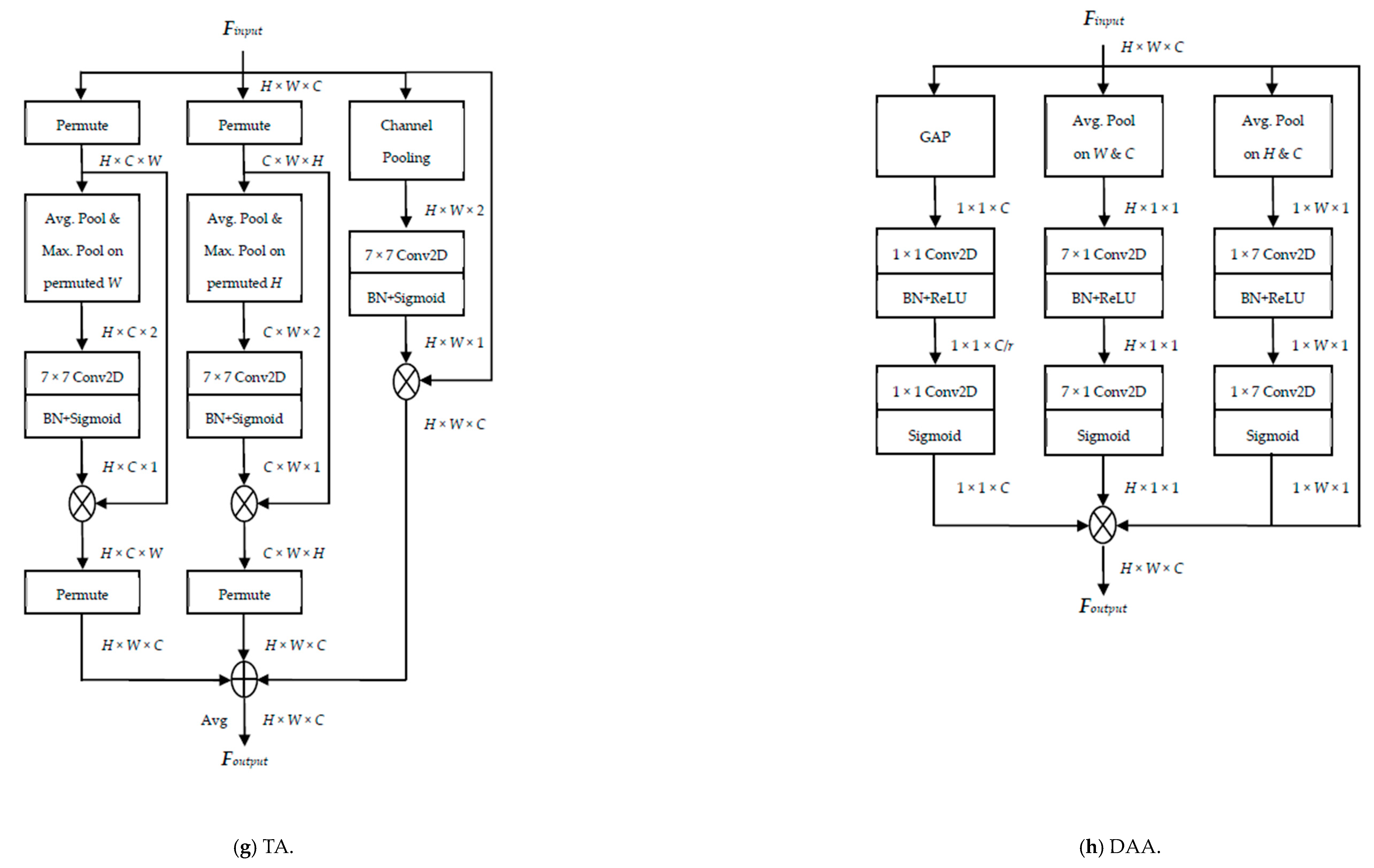
Attention modules can extract informative details from an image region, thus enriching the representation power of the overall model. Basically, there are two types of attentions. Channel attention focuses on ‘what’ is important, given different feature maps from an input image. Conversely, spatial attention addresses ‘where’ the position of the important region is [2]. Among these, some modules encode only informative channel details, such as SE [3] and ECA [4]. On the other hand, other modules complement the channel with spatial information, namely CBAM [2], ECBAM [12], CA [5], SCA [13], TA [6], and DAA [14]. Given F i n p u t R H × W × C and F o u t p u t R H × W × C as the input and output tensors, respectively, each attention module is briefly presented and discussed as follows: Note that H, W, and C represent those tensors’ height, width, and channel. Regarding these notations, the outlines for all the attention modules are depicted in Figure 1. Other acronyms in Figure 1 include ‘GAP’ and ‘GMP’, which refer to the Global Average Pooling and Global Max Pooling, respectively, while ‘BN’ stands for Batch Normalization. In addition, ‘Channel Pool’ is the abbreviation for channel pooling, ‘Concat.’ is the abbreviation for concatenation, and ‘Avg. Pool’ and ‘Max. Pool’ refer to the average pooling operation and maximum pooling operation, respectively. These pooling operations are performed in single or double dimensions, as indicated by H, W, or C, respectively. Finally, notation represents element-wise multiplication, whereas represents element-wise summation.
The SE [3] module was introduced to capture channel-wise relationships and choose the best representation by means of recalibrating the channel weight. Specifically, the squeeze operation aggregates information across spatial dimensions through GAP, while the excitation operation utilizes reduction ratio r to scale the channel dimension. With the aim of reducing complexity through 1D convolution, ECA [4] was developed to capture cross-channel interactions. Unlike SE, the dimensionality reduction operation was excluded from ECA to generate appropriate and feasible channel attention maps.
Instead of only attaining a channel-wise relationship, such as those in SE and ECA, CBAM [2] further improved the representational power by combining both channel and spatial attention modules in a sequence. The channel attention of CBAM was almost similar to that of SE, except that there were two pooling operations at the initial stage, namely GAP and GMP. On the other hand, spatial attention involved applying average pooling and max pooling on the channel dimension, which is collectively known as channel pooling. Furthermore, ECBAM [12] was conceived to extract channel and spatial information in a more robust way. Different from CBAM, which adopted SE as the channel attention, ECBAM utilized ECA with both GAP and GMP operations. In addition, ECBAM followed the same spatial attention setting as that of CBAM.
Considering the importance of positional information, CA [5] was introduced. Since convolution only extracts local information, as observed in the computation of spatial attention in CBAM and ECBAM modules [5], CA was suggested to overcome this problem by capturing long-range interactions. Similar to CA, SCA [13] was developed to fuse the channel attention maps with spatial information in two branches. With this arrangement, SCA aimed to capture cross-dimensional information from each branch simultaneously. As it is different from other attention modules, the pooling operation was omitted from SCA to preserve more information.
Instead of capturing attention with single branch (SE, ECA, CBAM, and ECBAM) or two branches arranged in parallel (CA and SCA), a module with three parallel branches known as TA [6] was introduced. TA was developed to capture the interdependencies between the channel and spatial dimensions concurrently. Akin to SCA, cross-dimensional interactions were captured by both channel branches, which were encoded with either height or width information. The remaining third branch adopted the same operating procedure as that of spatial attention in CBAM. Another three-branch structure arranged in parallel, known as DAA [14], was developed. Each of the three branches encoded information in the height, width, and channel dimensions separately. Unlike TA, which incorporated inter-dependency relationships, DAA built intra-dependencies for each dimension of the input tensor.
According to the respective authors, all the aforementioned attention modules [2,3,4,5,6,12,13,14] have lightweight characteristics. In addition, most of the attention modules, such as SE, ECA, CBAM, CA, TA, and DAA, were initially proposed for general ImageNet [7] classification and object detection applications. On the other hand, SCA was developed solely for ImageNet classification, while ECBAM was intended for face recognition tasks only. Although SE, ECA, and CBAM were originally introduced for image classification and object detection applications, there are other works [33,34,35] that incorporate these attention modules in face recognition tasks. The justification might be that these modules learn important face features through enhancement [33] of the channel attention or along with spatial attention. Another reason is that from the reported results of the corresponding works [33,34], the model incorporated with the attention module had a better performance compared to those of the baseline or model without the attention module.

3. Proposed Approach

A triplet-branch Low-Complexity Attention Module, known as LCAM, is proposed. Figure 2 shows the graphical outline for LCAM. The input and output tensors for LCAM are denoted as F i n p u t and F o u t p u t , respectively, where both tensors have the same spatial (H and W) and channel (C) dimensions. Notably, LCAM has three parallel branches, where each branch encodes information in the height, width, and channel dimensions, respectively.
Compared to those of TA and DAA, each branch of LCAM consists of only one convolution operation, as well as a smaller kernel size. Consequently, the number of FLOPs and parameters is reduced, yielding lower complexity and fewer memory requirements. Figure 3 shows a detailed block structure of LCAM, where the entire operations for LCAM can be summarized as:
F o u t p u t = F H F W F C F i n p u t
where F H , F W , and F C are the weighted attention map for the vertical, horizontal, and channel branches, respectively. In the following subsections, the details for each of the three branches are presented and discussed with respect to the graphical outline and block structure of LCAM.

3.1. Channel Attention Branch

The first unit of LCAM is the Channel Attention Branch (CAB), which exploits the inter-channel interaction of different feature maps. Motivated by ECA, additional batch normalization is appended in between the 1D convolution and sigmoid activation function to promote stability and facilitate the training process. Unlike DAA, the reduction ratio is not applied in the channel branch of LCAM. In this way, more effective channel attention can be learned while preserving channel information.
First, GAP is performed on the input tensor F i n p u t . Hence, a pooling feature, F G A P , with 1 × 1 × C dimension is generated. Next, a 1D convolution with adaptive kernel size is deployed to capture cross-channel interaction. Following ECA [4], the kernel size for 1D convolution is adaptively determined by:
k = | log 2 C + g γ | o d d
where g and γ are hyperparameters assigned, respectively, with values of 1 and 2. Moreover, | k | o d d represents the nearest odd number of kernel size. Note that the adaptive kernel size for LCAM is set to be at least 3. In essence, the predicted attention for each channel is based on a local k neighborhood. Finally, the channel attention map F C is obtained by applying sigmoid activation function to scale the weight for each channel. The whole process of CAB can be mathematically formulated as follows:
F G A P = 1 H × W h = 1 H w = 1 W F i n p u t ( h , w , c )
and
F C = σ ( b ( f 1 d k ( F G A P ) ) )
where f 1 d k denotes 1D convolution with the kernel of size k, which is determined adaptively by Equation (2), b is the batch normalization operation, and σ indicates the sigmoid activation function.

3.2. Vertical Attention Branch

With the intention to encode height information in the spatial dimension, the Vertical Attention Branch (VAB) is the second unit of LCAM. As opposed to other attention modules with 2D symmetric convolution, LCAM utilized only a 1D asymmetric convolution in each spatial branch. This approach helps in reducing the computational complexity and memory footprint. Moreover, LCAM capitalizes fully on the spatial information in every 1D asymmetric convolution operation. Hence, LCAM is not susceptible to information loss because more information can be preserved. Specifically, average pooling is performed on the channel dimension while retraining both the height and width information. Moreover, permutation operations also improve the robustness of face pose variations, which leads to a better face recognition performance.
Initially, the channel dimension of the input tensor is compressed through the channel average pooling operation. The generated pooling feature F C A P has a shape of H × W × 1. After that, the pool feature is permuted with respect to the height dimension. Intuitively, this operation involved rotation along the height dimension, which caused the swapping of positions between the width and channel dimensions. As a result, the dimension of the permuted feature F P H is rearranged to H × 1 × W. Subsequently, a 1D asymmetric convolution with a kernel of size 3 × 1 followed by a sigmoid activation function is deployed. The convoluted feature F C P H has a dimension of H × 1 × 1. Finally, another permutation operation is implemented to rotate the feature back to the original position. The generated attention map F H can then be used to calibrate the height dimension. In essence, the aforementioned steps can be mathematically summarized as:
F C A P = 1 C c = 1 C F i n p u t ( h , w , c )
F P H = p h ( F C A P )
F C P H = σ ( b ( f 3 × 1 ( F P H ) ) )
F H = p h ( F C P H )
where p h represents permutation operation along the height dimension, while f 3 × 1 corresponds to 3 × 1 asymmetric convolution.

3.3. Horizontal Attention Branch

Another counterpart unit for spatial dimension in LCAM is the Horizontal Attention Branch (HAB). The purpose of the HAB is to capture the width information. The workflow of the HAB is almost similar to that of the VAB, with some minor adjustments. Instead of permutation along the height dimension, the rotation operation of the HAB is carried out pertaining to the width dimension. In addition, 1 × 3 asymmetric convolution is utilized for the permuted feature.
Akin to VAB, the workflow of the HAB starts with the channel average pooling operation. Next, the pooling feature F C A P is rotated along the width dimension to yield a permuted feature, F P W , with a shape of 1 × W × H. Then, a 1D asymmetric convolution of 1 × 3 kernel size is utilized before appending a batch normalization and sigmoid activation function. Hence, a convoluted feature, F C P W , with a dimension of 1 × W × 1 is generated. Finally, the feature is rearranged to the original position through permutation operation. The entire flow of the HAB is first represented by Equation (5), while the subsequent steps are given as:
F P W = p w ( F C A P )
F C P W = σ ( b ( f 1 × 3 ( F P W ) ) )
F W = p w ( F C P W )
where p w refers to the permutation operation along the width dimension, while f 1 × 3 is the 1 × 3 asymmetric convolution.

4. Experiments and Analysis

In this section, the training and evaluation datasets for LCAM and previous attention modules are initially introduced. Next, experimental settings for all these modules are presented. Then, ablation studies are conducted to access the most suitable design structure for the LCAM module. After that, quantitative analysis is implemented to evaluate the verification accuracy. Finally, qualitative analysis is performed on the output images by visual inspection.

4.1. Dataset

All the models in this work employ UMD Faces [36] as the training dataset. There are around 367,888 face images of 8277 individuals in this medium-sized dataset. In comparison with other similar-sized datasets, such as CASIA WebFace [37] and VGGFace [38], the images of UMD Faces contain more pose variations, which facilitate the learning capability of a model. Face images with 112 × 112 × 3 dimensions are used for training. These faces are detected and aligned with a multi-task cascaded convolutional network (MTCNN) [20], which is available from Face.evoLVe library [39].
The efficiency of each model is evaluated through seven image-based and two additional template-based face datasets. The seven image-based datasets are LFW [40], CALFW [41], CPLFW [42], CFP-FF [43], CFP-FP [43], AgeDB-30 [44], and VGG2-FP [45]. All the image-based datasets are evaluated with pairwise face verification accuracy. Derived from IARPA Janus Benchmarks (IJB), two template-based datasets, specifically IJB-B [46] and IJB-C [47], are employed. The performances for IJB-B and IJB-C datasets are accessed through True Accept Rates (TAR) at False Accept Rates (FAR) of 0.001, 0.0001 and 0.00001.

4.2. Experimental Settings

The effectiveness and adaptability of LCAM and the previous eight attention modules discussed in Section 2.3 are evaluated by plugging them into three different lightweight face recognition models. Notably, this is carried out by evaluating the verification accuracies with respect to seven image-based and two template-based face recognition datasets, as mentioned in Section 4.1. These three lightweight face recognition models are ConvFaceNeXt [11], MobileFaceNet [8], and ProxylessFaceNAS [10]. Note that the attention module is placed in the rear position after the core building block of a model. Following previous works [5,14], the reduction ratios for SE, CBAM, CA, and DAA are fixed, respectively, at 24, 24, 32, and 8 to ensure similar model complexities.
All experiments are conducted with the TensorFlow framework on an Nvidia Tesla P100 GPU. Stochastic Gradient Descent optimizer is used to train these models from scratch. Moreover, a momentum of 0.9 and a weight decay of 0.0005 are employed. Additionally, a cosine learning schedule with an initial value of 0.1 and a decreased factor of 0.5 are adopted. Note that ConvFaceNeXt and MobileFaceNet are trained with a batch size of 256 for 49 epochs. Conversely, the batch size for ProxylessFaceNAS is 64 due to the GPU memory limitation. Furthermore, the loss function used for all models is ArcFace [48], which boosts the discriminative power of learned face features through the additive angular margin m. Given a feature xi belonging to identity class yi, ArcFace is formulated as:
L = 1 N i = 1 N ln e h ( cos ( θ y i + m ) ) e h ( cos ( θ y i + m ) ) + j = 1 , j y i C e h cos ( θ j )
where N is the batch size, C is the total number of classes in the training dataset, h is the scaling hyperparameter, and θ y i is the angle between the feature x i and i-th class center.

4.3. Ablation Studies

In this section, the optimum design structure and configuration for LCAM are studied. These evaluations are measured in terms of performance, FLOPs, and parameters. Among the four family members of ConvFaceNeXt, the base model selected to conduct all the experiments is ConvFaceNeXt_PE. This model will be referred to as ConFaceNeXt in the following sections for simplicity. Three sets of experiments are carried out based on the hill climbing technique [49]. First, the effect of different kernel sizes in the 1D asymmetric convolution of LCAM is accessed. Second, the influence of each of the three branches of LCAM, along with different combinations, is examined. Finally, the impact of different location configurations of LCAM in ConvFaceNeXt is investigated. The overview for these three sets of experiments is shown in Figure 4.

4.3.1. Effect of Different Kernel Size

Generally, most of the attention modules operate on 2D symmetric convolution. Hence, 1D asymmetric convolution is deployed in each of the vertical and horizontal branches of LCAM to reduce the computational complexity. As they are different from DAA, each of these branches exploits spatial information to the fullest extent. This is made possible by the permutation operation, which enables 1D asymmetric convolution to operate on both height and information. Four experiments with different kernel sizes are conducted. This analysis involves kernel sizes of three, five, seven, and nine. The verification accuracies for various kernel sizes are reported in Table 1 and Table 2 and Figure 5. Note that the first model with LCAM, which operates on a kernel of size three for 1D asymmetric convolution, is known as ConvFaceNeXt_LCAM. The subsequent models, which incorporate LCAM with kernel sizes of five, seven, and nine, are denoted as ConvFaceNeXt_L5K, ConvFaceNeXt_L7K, and ConvFaceNeXt_L9K, respectively.
From the results of the image-based dataset in Table 1, it can be seen that ConvFaceNeXt_LCAM and ConvFaceNeXt_L5K perform similarly well. However, when the kernel size is increased further to seven and nine, there is a drop in the verification accuracy. Note that DAA adopts 1D asymmetric convolution with a kernel of size seven for performance gain in the ImageNet classification task. Nevertheless, from the conducted experiments, it was observed that larger kernel sizes of seven and nine led to a performance deterioration in the face recognition task. This suggests that the performance tends to be saturated beyond the kernel of size five for evaluation using face datasets. Another possible reason might be that DAA is plugged into MobileNetV2 with a large (224 × 224 × 3) input image, while it was only 112 × 112 × 3 for ConvFaceNeXt.
Other lightweight face recognition models, such as MobileFaceNet and ProxylessFaceNAS, are fed with the same small input image size of 112 × 112 × 3 to reduce the computational complexity. In this situation, a smaller kernel size for 1D asymmetric convolution is more prone to extract local face information compared to that of a large kernel size. Although there is a 0.05% minor performance gain when one is switching from the kernel sizes of three to five, this increment is negligible compared to the additional 45 K parameters introduced by the model with a larger kernel size. In addition, as indicated in Table 2 and Figure 5 for template-based datasets, ConvFaceNeXt_LCAM with a kernel size of three performs better than the other models with larger kernel sizes do. Based on these results and the intention to propose a low-complexity attention module, a kernel of size three is adopted for LCAM to ensure more detailed and minute face features can be extracted.

4.3.2. Effect on Different Combination of Branches

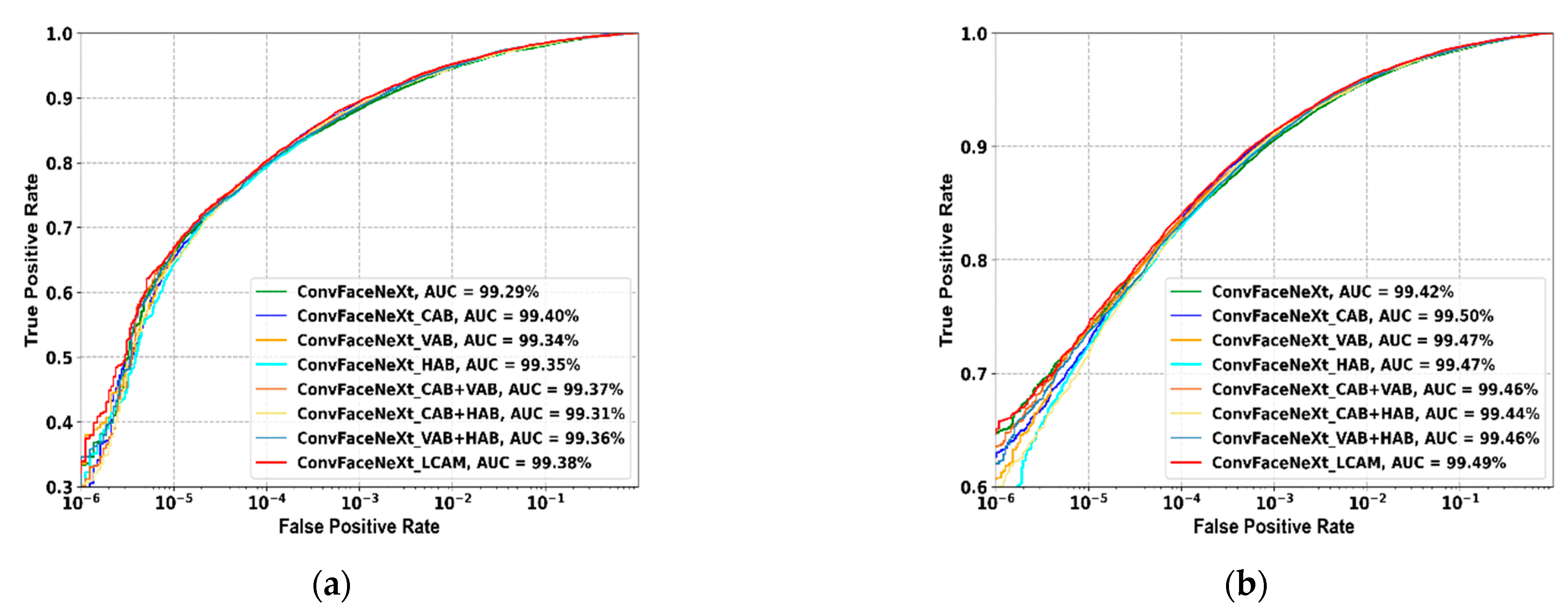
In this section, experiments are conducted to determine the optimum combination of branches for LCAM. Based on three branches of LCAM, namely CAB, VAB, and HAB, the effectiveness of seven different combinations is examined. These seven variations include three single-branch modules, three double-branch modules, and a triplet-branch module. Specifically, the first to the third models incorporate single branch modules, including ConFaceNeXt_CAB (channel), ConFaceNeXt_VAB (height), and ConFaceNeXt_HAB (width). Next, the fourth to the sixth models are integrated with double branch modules, namely ConFaceNeXt_CAB+VAB, ConFaceNeXt_CAB+HAB, and ConFaceNeXt_VAB+HAB. Finally, the last model comprises all three branches, denoted as ConvFaceNeXt_LCAM. Note that the baseline model is represented as ConvFaceNeXt. The results of applying different combinations of branches are shown in Table 3 and Table 4 and Figure 6.
It is observed that the model ConvFaceNeXt_LCAM with all three branches has the best overall performance for the image-based dataset, as shown in Table 3. In addition, the parameters for ConvFaceNeXt_LCAM are almost similar to those of the other variations, with a 0.5% slight increase in FLOPs compared to that of the baseline model. This implies that the combination of CAB, VAB, and HAB in LCAM is capable of improving the face verification performance. This is because the scaling weight of each dimension is highlighted properly. Hence, channel, height, and width (spatial) information can be captured effectively by LCAM. In addition, the remaining six models derived from LCAM improve the verification performance of the image-based dataset compared to that of the baseline model. For the single branch module, ConvFaceNeXt_CAB and ConvFaceNeXt_VAB show comparable performances, while ConvFaceNeXt_HAB has mediocre performance.
Meanwhile, among the three double-branch modules, ConvFaceNeXt_CAB+HAB performs better than the other two do. From the perspective of channel and width dimensions, there is a gradual performance improvement from the utilization of single to all three branches in LCAM. Concretely, when the models consider only a single branch with CAB or HAB, the verification accuracies are, respectively, 92.84% and 92.65%. When two branches are incorporated, as in the combination of CAB and HAB, the performance value increases to 93.00%. Eventually, the best result of 93.13% is obtained by integrating all three branches. Additionally, ConvFaceNeXt_LCAM accomplishes the highest accuracy for the template-based dataset, as shown in Table 4. These observations prove that it is crucial to combine all three branches to effectively recalibrate each dimension.

4.3.3. Effect on Different Integration Strategy

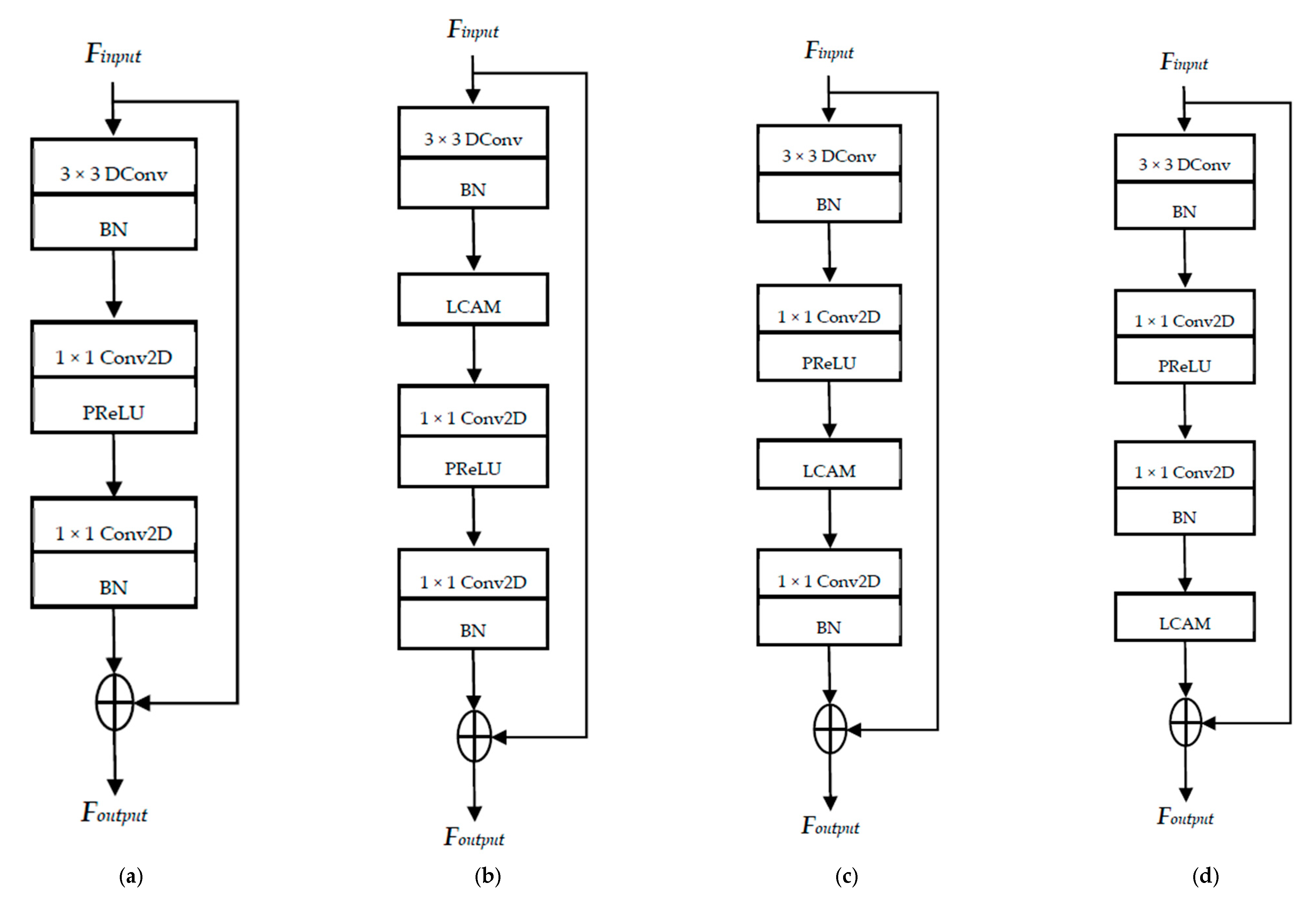
In order to gain insight into the optimum location for LCAM in the core building block of ConvFaceNeXt, several integration strategies are investigated. As a brief introduction, ECN is the main building block for ConvFaceNeXt with three convolution operations, as shown in Figure 7a. The ECN block starts with a depthwise convolution, followed by two pointwise convolutions. Note that the first pointwise convolution is used for channel expansion, while the second one is for channel reduction. Three variants of integration strategies are studied. The first ConvFaceNeXt_D1 model consists of integrating LCAM after depthwise convolution along with the batch normalization operation. The second ConvFaceNeXt_P1 model incorporates LCAM next to the first pointwise convolution along with the PReLU activation function. Finally, the last model, ConvFaceNeXt_LCAM, deploys the attention module at the end of an ECN block. For better clarity, these three variants are depicted in Figure 7b–d, where the structure for LCAM is shown in Figure 2.
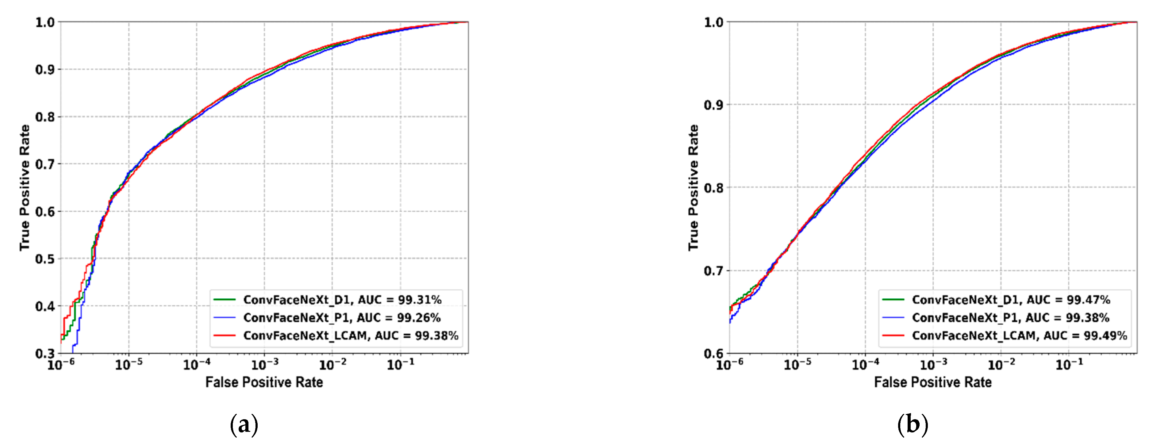
Through the reported results in Table 5 and Table 6, ConvFaceNeXt_LCAM has the best verification accuracy for almost all the datasets. One reason for this performance gain might be due to the placement of LCAM at the rear bottom position of an ECN block. Specifically, this placement ensures a richer feature representation because information can be fully extracted by all three convolution layers in the ECN block. In contrast, the convolution operation is performed only once or twice prior to the attention module in ConvFaceNeXt_D1 and ConvFaceNeXt_P1, respectively, leading to suboptimal information extraction. As an assumption, the verification accuracy of ConvFaceNeXt_P1 is supposed to be better than that of ConvFaceNeXt_D1 based on the intuition that more information can be encoded by using more convolution layers. However, this is not the case, as the performance of ConvFaceNeXt_P1 with two convolution operations prior to plugging the attention module is lower than that of ConvFaceNeXt_D1 with one convolution operation.
Upon closer observation, LCAM is integrated after the PReLU activation function for ConvFaceNeXt_P1. Contrarily, the integration of the attention module for ConvFaceNeXt_D1 and ConvFaceNeXt_LCAM occurs after the batch normalization operation, which yields a better performance. This observation suggests that the nonlinear activation function causes information loss to a certain extent [25]. Moreover, ConvFaceNeXt_P1 with the attention module placed after the first pointwise convolution has more complexity than those of the other two models. This is because the channel expansion induced by the first pointwise convolution inevitably increases the number of parameters in the corresponding attention module. Apart from that, ConvFaceNeXt_LCAM performs equally well for the template-based datasets, as shown in Table 6 and Figure 8. With respect to the aforementioned reasons, the attention module is thus integrated at the end of the core building block.

4.4. Quantitative Analysis

In this section, the experimental results for all attention modules are reported. Based on the ablation study, LCAM adopts the optimum settings shown in Section 4.3. This section further reviews the adaptability of LCAM to suit three different lightweight face recognition models, namely ConvFaceNeXt [11], MobileFaceNet [8], and ProxylessFaceNAS [10]. Specifically, the performances of each model plugs with LCAM or other attention modules are examined. Basically, a performance bias tends to occur when one is comparing models utilizing different training and testing datasets. For the sake of fairness, all the models incorporated with different attention modules are trained from scratch using the UMD face dataset with the experiment settings presented in Section 4.2. These models are then evaluated on seven image-based and two template-based face datasets, as described in Section 4.1.
With the aim of reducing the computational complexity, the ECN block is deployed as the core structure for ConvFaceNeXt. Moreover, blocks with the same output dimension are aggregated for a comprehensive feature correlation. The results of the ConvFaceNeXt plug with different attention modules are reported in Table 7 and Table 8. For image-based datasets, the verification accuracies are based on seven face datasets, where the average accuracy for each attention module is computed and shown in the last column of Table 7. Based on a brief glimpse at the average accuracy, it appears that all of the attention modules play an important role in increasing the performance results as compared to that of the baseline model with no attention mechanism. This conforms to the fact that attention modules increase the representational power of a neural network in general, and specifically, for lightweight face recognition models as well. Typically, modules combining both channel and spatial attentions perform much better than those with single-channel attention do. For example, models integrated with channel attention, such as SE and ECA, have lower average accuracy in contrast to those of SCA, TA, DAA, and LCAM, which consider both attentions. This proves that both attentions complement each other for richer channel and spatial representations.
With respect to the arrangement mode for channel and spatial attentions, it is observed that the parallel arrangements of SCA, TA, DAA, and LCAM yield better results as opposed to those of CBAM and ECBAM with sequential channel-spatial configuration. This validates the superiority of factorizing the attention module into several parallel branches for effective attention map generation. In terms of complexity, models with channel attention have lower FLOPs and similar parameters in comparison with those of other models with both attentions. However, this low complexity comes with a cost of a suboptimal performance. It is interesting to note that besides having the highest average accuracy with image-based datasets, the performance improvement of LCAM is achieved with the lowest FLOPs among the models that integrate both channel and spatial attentions. For template-based datasets, the performance for LCAM is among the best, as indicated by the verification accuracies in Table 8. As a whole, ConvFaceNeXt incorporates the LCAM attention module and has the best overall result, taking into account the accuracies, as well as parameters and FLOPs counts.
The core structure of MobileFaceNet is an inverted residual block. The performances of each MobileFaceNet integration with different attention modules are shown in Table 9 and Table 10. Likewise, all attention modules plugged into MobileFaceNet have the tendency to achieve better performance improvements compared to that of the baseline model. Several modules with both attentions, particularly ECBAM, TA, DAA, and LCAM, outperform the SE and ECA module with a single attention mechanism. Another notable observation is that although ECA, ECBAM, and LCAM utilize almost similar channel attentions, the spatial attention of ECBAM, as well as the Vertical and Horizontal Attention Branches of LCAM, contribute towards a better performance. The same condition can be perceived from SE and DAA modules, which adopt nearly identical channel attentions.
In terms of arrangement modes, the parallel combination of TA, DAA, and LCAM surpasses the performance of sequential combination in CBAM and ECBAM. Among these three parallel branches’ attention modules, LCAM attains the highest average accuracy. This validates the benefits of using only one convolution operation for each branch and fully exploiting the height and width information for every spatial branch in LCAM. Intriguingly, LCAM is accurate despite face pose variations, as observed by the highest accuracy value for CPLFW and VGG2-FP, in addition to the next best result for CFP-FP. From the comparison of modules with both attentions, LCAM has the least complexity in terms of FLOPs without sacrificing the verification performance, which is notably the best. In addition, with reference to the results in Table 10, the performance for LCAM is among the best for the template-based datasets. This proves that LCAM is well adapted to the MobileFaceNet architecture.
With the purpose of learning discriminative face features, an efficient model known as ProxylessFaceNAS is suggested. The core structure of ProxylessFaceNAS is an inverted, residual block. Note that for ProxylessFaceNAS, the expansion ratio and kernel size for the block are larger than those of ConvFaceNeXt and MobileFaceNet. Consequently, ProxylessFaceNAS is the largest or heaviest among the three baseline models. The results for ProxylessFaceNAS, attached with various attention modules, are shown in Table 11 and Table 12. For the image-based datasets, all the models with attention modules have better performances than the baseline model does, as shown in Table 11. Among these modules, TA, ECBAM, and LCAM outperform the others in terms of average verification accuracy. In addition, these three modules, with both attentions, outdo SE and ECA with only channel attention. In comparison with ECA, the spatial attention of ECBAM and LCAM contribute by complementing the channel attention for performance improvements. Moreover, in the context of ProxylessFaceNAS, ECBAM with sequential arrangement has a similar performance to those of LCAM and TA with the parallel arrangement.
Another interesting observation is that for those modules without a reduction ratio, the performance is superior as opposed to that of their corresponding counterpart with a reduction ratio. Specifically, the average verification accuracies for ECA, ECBAM, and LCAM are higher compared to those of SE, CBAM, and DAA, respectively. The reason is that some information might be lost due to dimensionality reduction when they are applying a reduction ratio in channel attention. Besides the higher gain, the computation costs for models integrated with ECA, ECBAM, and LCAM are lower, which suits the requirement of lightweight face recognition models. Although the average accuracy of TA is comparatively better than that of LCAM, this comes at the cost of more computational complexity. Concretely, for modules with both attentions, TA has the highest number of FLOPs, while LCAM has the least of them. For template-based datasets, LCAM achieves a superior performance in comparison with those of other attention modules, as shown in Table 12. These results demonstrate the flexibility of LCAM to perform well, not only in smaller ConvFaceNeXt and MobileFaceNet models, but in larger lightweight face recognition models such as ProxylessFaceNAS as well.
In essence, LCAM is robust and can be plugged into any lightweight face recognition model for a more accurate and superior feature representation compared to those of the other attention modules. This shows that LCAM has great adaptability without worsening the performance. This is evidenced by the highest average verification accuracy for image-based datasets when one is integrating LCAM in ConvFaceNeXt and MobileFaceNet. For ProxylessFaceNAS, LCAM performs equally well with comparable results to those of TA, albeit with much lower complexity. With regard to template-based datasets, LCAM again shows a good and competitive performance measured by verification accuracies.

4.5. Qualitative Analysis

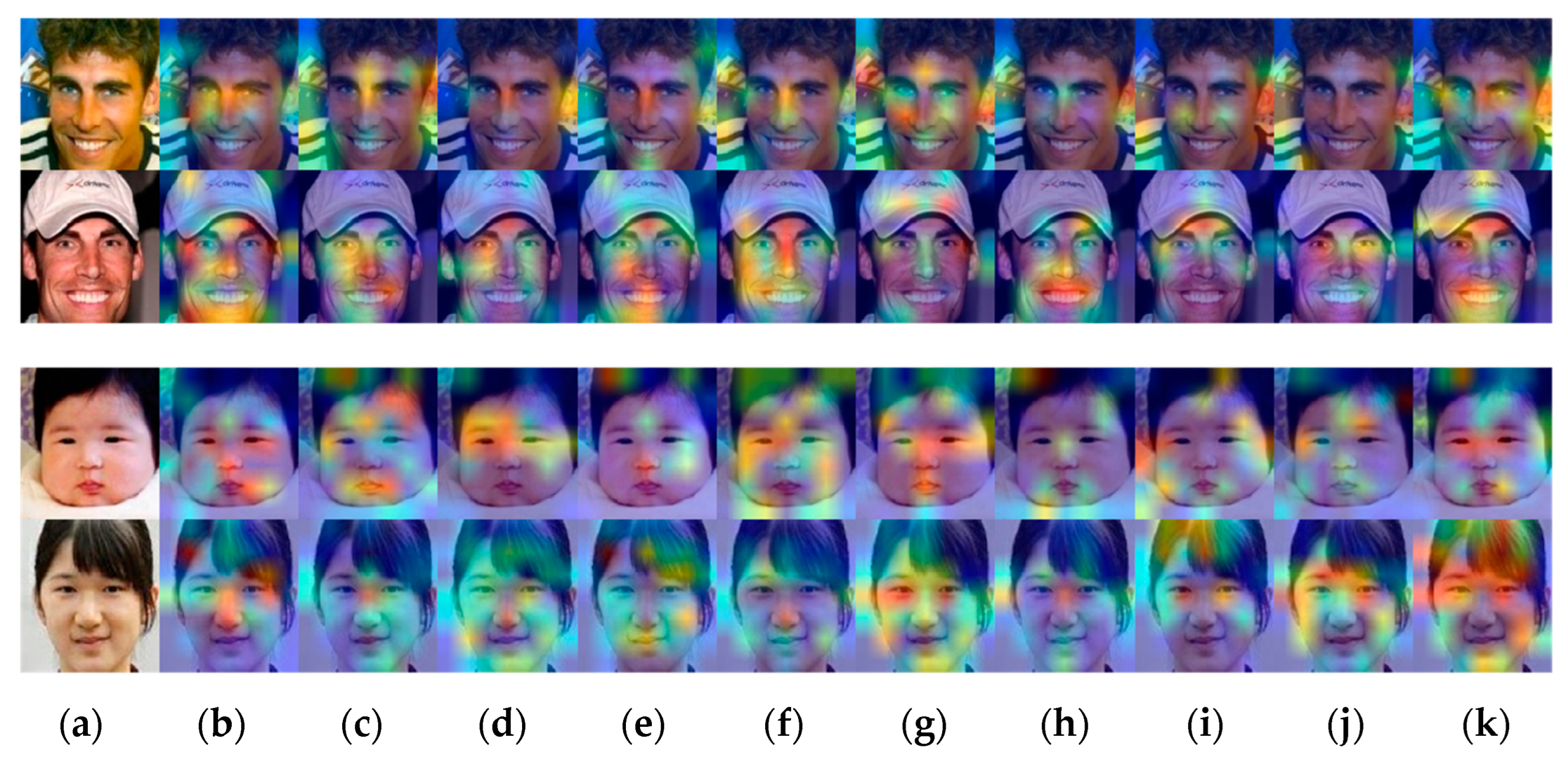
In this section, the Grad-CAM [50] technique is used to visualize the effectiveness of the proposed LCAM attention module in recognizing and localizing important facial features, thus enhancing the model’s representational power. Note that the color scales for Grad-CAM rank from red at the top to green, and finally, to blue to indicate the most and least significant regions, respectively. Random examples of positive face image pairs are taken, which correspond to the same individual. The visualization comprises the proposed LCAM and eight previous attention modules, which are all plugged into the ConvFaceNeXt model trained with the same dataset and settings as those described in Section 4.1 and Section 4.2.
Two pairs of face images from LFW are shown in Figure 9. The first pair shows the faces of a lady from the front. For the top face image, LCAM can highlight the eyes, mouth, and ears properly. Note that it is vital to distinguish discriminative face parts such as the eyes, nose, mouth, and ears for face recognition tasks [51]. Although CA exhibits a similar ability to emphasize those face parts, unnecessary regions encompassing the whole upper hair area are excited as well. Some other attention modules, such as SE and ECBAM, are observed to perform excitation only on the eye parts. Similarly, ECA and TA focus only on the ear parts. Even though the whole face region is covered by DAA, the level of excitation is lower on discriminative face parts. For the face image of the lady at the bottom, LCAM shows the most excitation, particularly on the eyes, nose, and ears, as shown in the orange and yellow regions. ECA and TA highlight the whole face region as well, albeit with less excitation. Other attention modules show a less strong response towards distinctive face parts.
The second image from the LFW dataset shows a frontal face of a guy. It is observed that LCAM has the capacity to locate discriminative face parts of the guy in both the top and bottom images. Although CA highlights the nose and mouth parts properly in the bottom image, the background regions are equally emphasized, which is not desirable. In addition, other attention modules, such as TA and DAA, only focus on the forehead and lower right part of the chin, with no emphasis given to discriminative face parts, as observed in the bottom face images.
Two additional cross-pose face images from CPLFW are shown in Figure 10. The first image shows the face of a guy from the front on top and a side view of his face on the bottom. On the front view image of the face, LCAM shows the most excitation on the eyes, nose, and mouth compared to that of the other attention modules. Similarly, TA highlights those parts despite with a less strong response towards the right eye and mouth. In contrast, other attention modules only focus on certain face regions, for example, CBAM and SCA, which focus on the less relevant forehead area. For the side-view image of the guy, LCAM shows more attentiveness to the eye and nose. DAA has comparable performance as well, while some other attention modules highlight face regions to a certain extent. The second pair consists of two side-view images of a lady. It is observed that LCAM can focus correctly on the face region in the top image. In addition, LCAM is the only method with a strong reaction to the nose tip on the bottom image. Although ECBAM is able to highlight most of the side face region on the right, discriminative face parts are neglected.
Lastly, two pairs of images of faces at different ages are shown in Figure 11. The image on the top corresponds to a face that is younger than the bottom one is. For the first pair, consisting of guy images, LCAM exhibits more excitation on the eyes and nose in comparison with those of the other attention modules, as illustrated by the images on the top. Likewise, CA yields an equivalent performance. In contrast, the excitation is especially poor for DAA on the face region, focusing instead on irrelevant background and shirt areas. For the bottom face image with a hat, LCAM again shows significant excitation on the eyes, nose, and mouth parts. Generally, other attention modules are able to highlight the face region, albeit with some of them having less excitation. The second pair represents the face of a girl. For the top image, discriminative face parts such as the eyes and mouth are well emphasized by LCAM and CA. Regarding the image on the bottom, LCAM shows more excitation on the face region, particularly on the eyes. Contrarily, other attention modules have less excitation or only highlight certain facial parts. For instance, TA only shows a response towards the eyes, while ignoring other discriminative parts.
Qualitative observations attest to LCAM’s superiority in not only highlighting face region, but also in emphasizing important face parts such as the eyes, nose, mouth, and ears. Concretely, these targeted parts play an important role in obtaining pose- and age-invariant features to boost the accuracy, as well as the overall performance of a model [52].

5. Conclusions

An attention module known as the Low-Complexity Attention Module (LCAM) is proposed for mobile-based networks in general, and specifically, for lightweight face recognition models. Basically, the LCAM consists of three parallel branches to encode scaling information in the channel, height, and width dimensions. In order to ensure low complexity, each of the LCAM branches utilizes only one convolution operation. Concretely, the Channel Attention Branch deploys a 1D convolution, while the other two Vertical and Horizontal Attention Branches employ, respectively, 1D asymmetric convolution. As a result, LCAM has fewer FLOPs and fewer parameters compared to those of other modules, which consider both channel and spatial attentions. Aside from that, although the Vertical Attention Branch and the Horizontal Attention Branch are separate entities, each of these branches makes full use of the height and width information through 1D asymmetric convolution. In this way, LCAM promotes information interaction within each spatial branch and minimizes the information loss. Several integral attributes of LCAM are examined in the ablation studies. First, 1D asymmetric convolution with a kernel size of three is adopted with the aim of extracting more detailed information. Second, a comprehensive attention module is obtained by combining all three branches of LCAM to improve the overall performance. Finally, LCAM is integrated at the rear of a core building block to ensure richer feature representations and low computational costs. In the quantitative analysis, LCAM achieved the highest verification accuracy among all the other attention modules, irrespective of the network model. Moreover, qualitative observation implies that LCAM is capable of highlighting face regions, while simultaneously emphasizing important face parts. Although LCAM shows a better performance, there are some limitations of the proposed module, which provide room for improvements. Specifically, pooling operations in the channel and spatial branches of LCAM might cause information loss to a certain extent. For instance, the global average pooling in the Channel Attention Branch could possibly cause a loss of spatial information, and vice versa, for the spatial attention branches. In future, mechanisms for further reducing information loss will be explored in LCAM, so as to achieve higher accuracy, while retaining important information, which is crucial for face recognition tasks. In addition, the performance of LCAM in other vision applications, such as object detection and semantic segmentation, will be analyzed in the future to investigate the generality of this attention module.

Author Contributions

Conceptualization, S.C.H., H.I., S.A.S. and T.F.N.; methodology, S.C.H. and H.I.; writing—original draft preparation, S.C.H.; writing—review and editing, H.I., S.A.S. and T.F.N.; supervision, H.I. and S.A.S.; funding acquisition, H.I. and T.F.N. All authors have read and agreed to the published version of the manuscript.

Funding

This research was funded by Universiti Sains Malaysia under Research University Grant 1001/PELECT/8014052.

Institutional Review Board Statement

Not applicable.

Informed Consent Statement

Not applicable.

Data Availability Statement

All the presented datasets in this paper can be found through the referenced papers.

Acknowledgments

The authors would like to thank everyone for their support during the implementation of this project, including Guowei Wang for valuable bits of advice, feedback, and the sharing of Keras insightface on https://github.com/leondgarse/Keras_insightface, accessed on 5 March 2022. In addition, S.C.H. would like to express gratitude to the Public Service Department of Malaysia, which offered the Hadiah Latihan Persekutuan (HLP) scholarship for this study.

Conflicts of Interest

The authors declare no conflict of interest.

References

  1. Guo, M.; Xu, T.; Liu, J.; Liu, Z.; Jiang, P.; Mu, T.; Zhang, S.; Martin, R.R.; Cheng, M.; Hu, S. Attention Mechanisms in Computer Vision: A Survey. Comp. Vis. Media 2022, 8, 331–368. [Google Scholar] [CrossRef]
  2. Woo, S.; Park, J.; Lee, J.; Kweon, I.S. CBAM: Convolutional Block Attention Module. In Proceedings of the European Conference on Computer Vision (ECCV), Munich, Germany, 8–14 September 2018; pp. 3–19. [Google Scholar] [CrossRef] [Green Version]
  3. Hu, J.; Shen, L.; Albanie, S.; Sun, G.; Wu, E. Squeeze-and-Excitation Networks. IEEE Trans. Pattern Anal. Mach. Intell. 2020, 42, 2011–2023. [Google Scholar] [CrossRef] [PubMed] [Green Version]
  4. Wang, Q.; Wu, B.; Zhu, P.; Li, P.; Zuo, W.; Hu, Q. ECA-Net: Efficient Channel Attention for Deep Convolutional Neural Networks. In Proceedings of the IEEE Computer Society Conference on Computer Vision and Pattern Recognition (CVPR), Seattle, WA, USA, 13–19 June 2020; pp. 11531–11539. [Google Scholar] [CrossRef]
  5. Hou, Q.; Zhou, D.; Feng, J. Coordinate Attention for Efficient Mobile Network Design. In Proceedings of the IEEE Computer Society Conference on Computer Vision and Pattern Recognition (CVPR), Nashville, TN, USA, 20–25 June 2021; pp. 13708–13717. [Google Scholar] [CrossRef]
  6. Misra, D.; Nalamada, T.; Arasanipalai, A.U.; Hou, Q. Rotate to Attend: Convolutional Triplet Attention Module. In Proceedings of the IEEE Winter Conference on Applications of Computer Vision (WACV), Waikoloa, HI, USA, 3–8 January 2021; pp. 3138–3147. [Google Scholar] [CrossRef]
  7. Deng, J.; Dong, W.; Socher, R.; Li, L.; Kai, L.; Fei-Fei, L. ImageNet: A Large-Scale Hierarchical Image Database. In Proceedings of the IEEE Computer Society Conference on Computer Vision and Pattern Recognition (CVPR), Miami, FL, USA, 20–25 June 2009; pp. 248–255. [Google Scholar] [CrossRef] [Green Version]
  8. Chen, S.; Liu, Y.; Gao, X.; Han, Z. MobileFaceNets: Efficient CNNs for Accurate Real-Time Face Verification on Mobile Devices. In Proceedings of the Chinese Conference on Biometric Recognition (CCBR), Urumqi, China, 11–12 August 2018; pp. 428–438. [Google Scholar] [CrossRef] [Green Version]
  9. Martínez-Díaz, Y.; Luevano, L.S.; Méndez-Vázquez, H.; Nicolás-Díaz, M.; Chang, L.; Gonzalez-Mendoza, M. ShuffleFaceNet: A Lightweight Face Architecture for Efficient and Highly-Accurate Face Recognition. In Proceedings of the IEEE International Conference on Computer Vision Workshop (ICCVW), Seoul, South Korea, 27–28 October 2019; pp. 2721–2728. [Google Scholar] [CrossRef]
  10. Martínez-Díaz, Y.; Nicolás-Díaz, M.; Méndez-Vázquez, H.; Luevano, L.S.; Chang, L.; Gonzalez-Mendoza, M.; Sucar, L.E. Benchmarking Lightweight Face Architectures on Specific Face Recognition Scenarios. Artif. Intell. Rev. 2021, 54, 6201–6244. [Google Scholar] [CrossRef]
  11. Hoo, S.C.; Ibrahim, H.; Suandi, S.A. ConvFaceNeXt: Lightweight Networks for Face Recognition. Mathematics 2022, 10, 3592. [Google Scholar] [CrossRef]
  12. Zhang, Y.; Wang, X.; Shakeel, M.S.; Wan, H.; Kang, W. Learning Upper Patch Attention using Dual-Branch Training Strategy for Masked Face Recognition. Pattern Recognit. 2022, 126, 1–15. [Google Scholar] [CrossRef]
  13. Liu, T.; Luo, R.; Xu, L.; Feng, D.; Cao, L.; Liu, S.; Guo, J. Spatial Channel Attention for Deep Convolutional Neural Networks. Mathematics 2022, 10, 1750. [Google Scholar] [CrossRef]
  14. Mo, R.; Lai, S.; Yan, Y.; Chai, Z.; Wei, X. Dimension-Aware Attention for Efficient Mobile Networks. Pattern Recognit. 2022, 131, 108899. [Google Scholar] [CrossRef]
  15. Shah, S.W.; Kanhere, S.S. Recent Trends in User Authentication—A Survey. IEEE Access. 2019, 7, 112505–112519. [Google Scholar] [CrossRef]
  16. Brown, D. Mobile Attendance based on Face Detection and Recognition using OpenVINO. In Proceedings of the International Conference on Artificial Intelligence and Smart Systems (ICAIS), Coimbatore, India, 25–27 March 2021; pp. 1152–1157. [Google Scholar] [CrossRef]
  17. Shaukat, Z.; Akhtar, F.; Fang, J.; Ali, S.; Azeem, M. Cloud-based Face Recognition for Google Glass. In Proceedings of the 2018 International Conference on Computing and Artificial Intelligence (ICCAI), Chengdu, China, 12–14 March 2018; pp. 104–111. [Google Scholar] [CrossRef]
  18. Hoo, S.C.; Ibrahim, H. Biometric-based Attendance Tracking System for Education Sectors: A Literature Survey on Hardware Requirements. J. Sens. 2019, 2019, 1–25. [Google Scholar] [CrossRef]
  19. Ranjan, R.; Sankaranarayanan, S.; Bansal, A.; Bodla, N.; Chen, J.C.; Patel, V.M.; Castillo, C.D.; Chellappa, R. Deep Learning for Understanding Faces: Machines May Be Just as Good, or Better, than Humans. IEEE Signal Process. Mag. 2018, 35, 66–83. [Google Scholar] [CrossRef]
  20. Zhang, K.; Zhang, Z.; Li, Z.; Qiao, Y. Joint Face Detection and Alignment Using Multitask Cascaded Convolutional Networks. IEEE Signal Process. Lett. 2016, 23, 1499–1503. [Google Scholar] [CrossRef] [Green Version]
  21. Najibi, M.; Samangouei, P.; Chellappa, R.; Davis, L.S. SSH: Single Stage Headless Face Detector. In Proceedings of the IEEE International Conference on Computer Vision (ICCV), Venice, Italy, 22–29 October 2017. [Google Scholar]
  22. Du, H.; Shi, H.; Zeng, D.; Zhang, X.P.; Mei, T. The Elements of End-to-end Deep Face Recognition: A Survey of Recent Advances. ACM Comput. Surv. 2022, 54, 1–42. [Google Scholar] [CrossRef]
  23. Wang, Z.; Chen, J.; Hu, J.; Wang, Z.; Chen, J.; Hu, J. Multi-View Cosine Similarity Learning with Application to Face Verification. Mathematics 2022, 10, 1800. [Google Scholar] [CrossRef]
  24. Deng, J.; Guo, J.; Zhang, D.; Deng, Y.; Lu, X.; Shi, S. Lightweight Face Recognition Challenge. In Proceedings of the IEEE International Conference on Computer Vision (ICCV), Seoul, Korea, 27 October–2 November 2019. [Google Scholar]
  25. Sandler, M.; Howard, A.; Zhu, M.; Zhmoginov, A.; Chen, L. MobileNetV2: Inverted Residuals and Linear Bottlenecks. In Proceedings of the IEEE Computer Society Conference on Computer Vision and Pattern Recognition (CVPR), Salt Lake City, UT, USA, 18–23 June 2018; pp. 4510–4520. [Google Scholar] [CrossRef] [Green Version]
  26. Ma, N.; Zhang, X.; Zheng, H.; Sun, J. ShuffleNet V2: Practical Guidelines for Efficient CNN Architecture Design. In Proceedings of the European Conference on Computer Vision (ECCV), Munich, Germany, 8–14 September 2018; pp. 122–138. [Google Scholar] [CrossRef] [Green Version]
  27. Howard, A.G.; Zhu, M.; Chen, B.; Kalenichenko, D.; Wang, W.; Weyand, T.; Andreetto, M.; Adam, H. MobileNets: Efficient Convolutional Neural Networks for Mobile Vision Applications. arXiv 2017, arXiv:1704.04861. [Google Scholar] [CrossRef]
  28. Cai, H.; Zhu, L.; Han, S. ProxylessNAS: Direct Neural Architecture Search on Target Task and Hardware. In Proceedings of the International Conference on Learning Representations (ICLR), New Orleans, LA, USA, 6–9 May 2019; pp. 1–13. [Google Scholar] [CrossRef]
  29. Liu, Z.; Mao, H.; Wu, C.; Feichtenhofer, C.; Darrell, T.; Xie, S. A ConvNet for the 2020s. In Proceedings of the IEEE Computer Society Conference on Computer Vision and Pattern Recognition (CVPR), New Orleans, LA, USA, 18–24 June 2022; pp. 11966–11976. [Google Scholar] [CrossRef]
  30. Abdulhussain, S.H.; Mahmmod, B.M.; AlGhadhban, A.; Flusser, J. Face Recognition Algorithm Based on Fast Computation of Orthogonal Moments. Mathematics 2022, 10, 2721. [Google Scholar] [CrossRef]
  31. Alzubaidi, L.; Zhang, J.; Humaidi, A.J.; Al-Dujaili, A.; Duan, Y.; Al-Shamma, O.; Santamaría, J.; Fadhel, M.A.; Al-Amidie, M.; Farhan, L. Review of Deep Learning: Concepts, CNN Architectures, Challenges, Applications, Future Directions. J. Big Data 2021, 8, 1–74. [Google Scholar] [CrossRef]
  32. Khan, S.; Rahmani, H.; Shah, S.A.A.; Bennamoun, M. A Guide to Convolutional Neural Networks for Computer Vision; Morgan & Claypool Publishers: San Rafael, CA, USA, 2018. [Google Scholar]
  33. Liu, W.; Zhou, L.; Chen, J. Face Recognition Based on Lightweight Convolutional Neural Networks. Information 2021, 12, 191. [Google Scholar] [CrossRef]
  34. Xiao, J.; Jiang, G.; Liu, H. A Lightweight Face Recognition Model based on MobileFaceNet for Limited Computation Environment. EAI Endorsed Trans. Internet Things 2022, 7, 1–9. [Google Scholar] [CrossRef]
  35. Li, X.; Wang, F.; Hu, Q.; Leng, C. Airface: Lightweight and Efficient Model for Face Recognition. In Proceedings of the 2019 IEEE/CVF International Conference on Computer VisionWorkshop (ICCVW), Seoul, Republic of Korea, 27–28 October 2019; pp. 2678–2682. [Google Scholar]
  36. Bansal, A.; Nanduri, A.; Castillo, C.D.; Ranjan, R.; Chellappa, R. UMDFaces: An Annotated Face Dataset for Training Deep Networks. In Proceedings of the IEEE International Joint Conference on Biometrics (IJCB), Denver, CO, USA, 1–4 October 2017; pp. 464–473. [Google Scholar] [CrossRef] [Green Version]
  37. Yi, D.; Lei, Z.; Liao, S.; Li, S. Learning Face Representation from Scratch. arXiv 2014, arXiv:1411.7923. [Google Scholar] [CrossRef]
  38. Parkhi, O.M.; Vedaldi, A.; Zisserman, A. Deep Face Recognition. In Proceedings of the British Machine Vision Conference (BMVC), Swansea, UK, 7–10 September 2015. [Google Scholar] [CrossRef] [Green Version]
  39. Wang, Q.; Zhang, P.; Xiong, H.; Zhao, J. Face.evoLVe: A Cross-Platform Library for High-Performance Face Analytics. Neurocomputing 2022, 494, 443–445. [Google Scholar] [CrossRef]
  40. Huang, G.B.; Mattar, M.; Berg, T.; Learned-Miller, E. Labeled Faces in the Wild: A Database for Studying Face Recognition in Unconstrained Environments. In Proceedings of the Workshop on Faces in ‘Real-Life’ Images: Detection, Alignment, and Recognition, Marseille, France, 12–18 October 2008. [Google Scholar]
  41. Zheng, T.; Deng, W.; Hu, J. Cross-Age LFW: A Database for Studying Cross-Age Face Recognition in Unconstrained Environments. arXiv 2017, arXiv:1708.08197. [Google Scholar] [CrossRef]
  42. Zheng, T.; Deng, W. Cross-Pose LFW: A Database for Studying Cross-Pose Face Recognition in Unconstrained Environments; Technical Report; Beijing University of Posts and Telecommunications: Beijing, China, 2018; Available online: http://www.whdeng.cn/CPLFW/Cross-Pose-LFW.pdf (accessed on 3 December 2022).
  43. Sengupta, S.; Chen, J.C.; Castillo, C.; Patel, V.M.; Chellappa, R.; Jacobs, D.W. Frontal to Profile Face Verification in the Wild. In Proceedings of the 2016 IEEE Winter Conference on Applications of Computer Vision (WACV), Lake Placid, NY, USA, 7–9 March 2016; pp. 1–9. [Google Scholar] [CrossRef]
  44. Moschoglou, S.; Papaioannou, A.; Sagonas, C.; Deng, J.; Kotsia, I.; Zafeiriou, S. AgeDB: The First Manually Collected, In-the-Wild Age Database. In Proceedings of the IEEE Conference on Computer Vision and Pattern Recognition Workshops (CVPRW), Honolulu, HI, USA, 21–26 June 2017; pp. 51–59. [Google Scholar] [CrossRef] [Green Version]
  45. Cao, Q.; Shen, L.; Xie, W.; Parkhi, O.M.; Zisserman, A. VGGFace2: A Dataset for Recognising Faces across Pose and Age. In Proceedings of the 2018 13th IEEE International Conference on Automatic Face & Gesture Recognition (FG 2018), Xi’an, China, 15–19 May 2018; pp. 67–74. [Google Scholar] [CrossRef] [Green Version]
  46. Whitelam, C.; Taborsky, E.; Blanton, A.; Maze, B.; Adams, J.; Miller, T.; Kalka, N.; Jain, A.K.; Duncan, J.A.; Allen, K.; et al. IARPA Janus Benchmark-B Face Dataset. In Proceedings of the IEEE Conference on Computer Vision and Pattern Recognition Workshops (CVPRW), Honolulu, HI, USA, 21–26 June 2017; pp. 592–600. [Google Scholar] [CrossRef]
  47. Maze, B.; Adams, J.; Duncan, J.A.; Kalka, N.; Miller, T.; Otto, C.; Jain, A.K.; Niggel, W.T.; Anderson, J.; Cheney, J.; et al. IARPA Janus Benchmark-C: Face Dataset and Protocol. In Proceedings of the 2018 International Conference on Biometrics (ICB), Queensland, Australia, 20–23 February 2018; pp. 158–165. [Google Scholar] [CrossRef]
  48. Deng, J.; Guo, J.; Yang, J.; Xue, N.; Cotsia, I.; Zafeiriou, S.P. ArcFace: Additive Angular Margin Loss for Deep Face Recognition. IEEE Trans. Pattern Anal. Mach. Intell. 2021, 44, 5962–5979. [Google Scholar] [CrossRef] [PubMed]
  49. Russell, S.; Norvig, P. Artifcial Intelligence: A Modern Approach, 4th Global ed.; Pearson Education Limited: London, UK, 2022. [Google Scholar]
  50. Selvaraju, R.R.; Cogswell, M.; Das, A.; Vedantam, R.; Parikh, D.; Batra, D. Grad-CAM: Visual Explanations from Deep Networks via Gradient-Based Localization. Int. J. Comput. Vis. 2020, 128, 336–359. [Google Scholar] [CrossRef] [Green Version]
  51. Zhao, J.; Han, J.; Shao, L. Unconstrained Face Recognition Using a Set-to-Set Distance Measure on Deep Learned Features. IEEE Trans. Circuits Syst. Video Technol. 2018, 28, 2679–2689. [Google Scholar] [CrossRef] [Green Version]
  52. Wang, Q.; Guo, G. LS-CNN: Characterizing Local Patches at Multiple Scales for Face Recognition. IEEE Trans. Inf. Forensics Secur. 2019, 15, 1640–1653. [Google Scholar] [CrossRef]
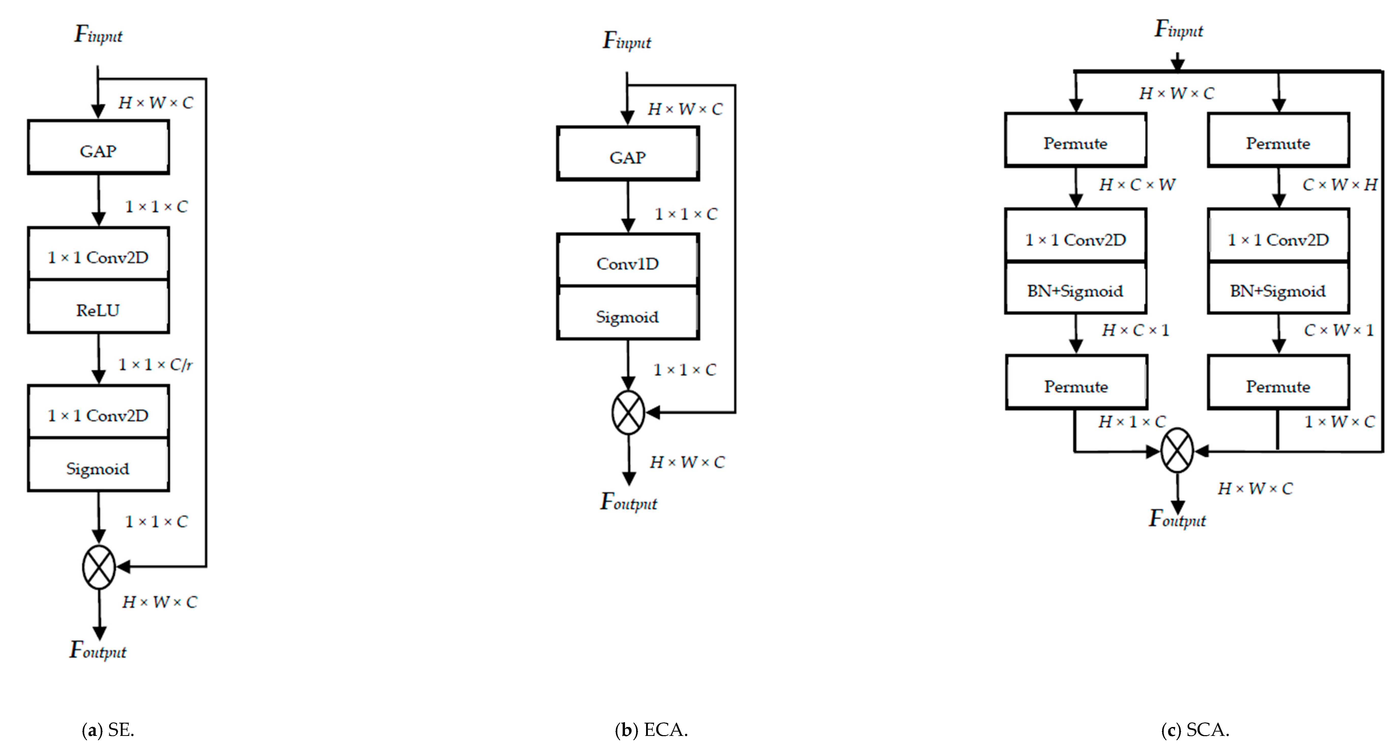
Figure 1. Graphical outlines of various attention modules. (a) SE [3]; (b) ECA [4]; (c) SCA [13]; (d) CBAM [2]; (e) ECBAM [12]; (f) CA [5]; (g) TA [6]; (h) DAA [14].
Mathematics 11 01694 g001aMathematics 11 01694 g001bMathematics 11 01694 g001c
Figure 2. Graphical outlines of the proposed LCAM.
Mathematics 11 01694 g002
Figure 3. LCAM framework illustrated with block structure. The three branches arrange from top to bottom are, respectively, Channel Attention Branch (CAB), Vertical Attention Branch (VAB), and Horizontal Attention Branch (HAB).
Mathematics 11 01694 g003
Figure 4. Flow chart illustrating experiments conducted based on hill climbing technique to tune and determine the optimum structure for LCAM.
Mathematics 11 01694 g004
Figure 5. ROC curves of 1:1 verification for different kernel sizes. (a) IJB-B dataset; (b) IJB-C dataset.
Mathematics 11 01694 g005
Figure 6. ROC curves on different combination of branches. (a) IJB-B dataset; (b) IJB-C dataset.
Mathematics 11 01694 g006
Figure 7. ECN building block with different integration strategies. (a) ECN block; (b) ECN block integrated with LCAM after the depthwise convolution along with batch normalization operation; (c) ECN block integrated with LCAM after the first pointwise convolution along with PReLU activation function; (d) ECN block integrated with LCAM at the end. Here, ‘DConv’ represents Depthwise Convolution, while ‘1 × 1 Conv2D’ represents pointwise convolution.
Mathematics 11 01694 g007
Figure 8. ROC curves on different integration strategies. (a) IJB-B dataset; (b) IJB-C dataset.
Mathematics 11 01694 g008
Figure 9. Two random face image pairs from the LFW [40] dataset. The original image pairs are shown in (a). Corresponding Grad-CAM visualization for the baseline pair is depicted in (b), and other attention modules are depicted from (cj), while the proposed attention module of this work is illustrated in (k), all are arranged column-wise from left to right. (a) Original face image pairs; (b) ConvFaceNeXt; (c) SE; (d) ECA; (e) CBAM; (f) ECBAM; (g) CA; (h) SCA; (i) TA; (j) DAA; (k) LCAM.
Mathematics 11 01694 g009
Figure 10. Two random face image pairs from CPLFW [42] dataset. The original image pairs are shown in (a). Corresponding Grad-CAM visualization for the baseline pair is depicted in (b), and other attention modules are depicted from (cj), while the proposed attention module of this work is illustrated in (k), all arranged column-wise from left to right. (a) Original face image pairs; (b) ConvFaceNeXt; (c) SE; (d) ECA; (e) CBAM; (f) ECBAM; (g) CA; (h) SCA; (i) TA; (j) DAA; (k) LCAM.
Mathematics 11 01694 g010
Figure 11. Two random face image pairs from CALFW [41] dataset. The original image pairs are shown in (a). Corresponding Grad-CAM visualization for the baseline pair is depicted in (b), and other attention modules are depicted from (cj), while the proposed attention module of this work is illustrated in (k), all arranged column-wise from left to right. (a) Original face image pairs; (b) ConvFaceNeXt; (c) SE; (d) ECA; (e) CBAM; (f) ECBAM; (g) CA; (h) SCA; (i) TA; (j) DAA; (k) LCAM.
Mathematics 11 01694 g011
Table 1. Performance results of different kernel sizes. These results are reported in terms of parameters, FLOPs, and verification accuracy for LFW, CALFW, CPLFW, CFP-FF, CFP-FP, AgeDB-30, and VGG2-FP. Moreover, the average accuracy for the seven image-based datasets is shown in the last column. (Bold values are the highest obtained values by the methods).
ModelParam. (M)FLOPs (M)LFWCALFWCPLFWCFP-FFCFP-FPAgeDB-30VGG2-FPAverage
ConvFace NeXt_LCAM1.05406.5699.2093.4786.4098.9089.4993.7090.7893.13
ConvFace NeXt_L5K1.05406.6099.2393.7386.9799.0189.6193.6590.0493.18
ConvFace NeXt_L7K1.05406.6599.1593.6786.3399.1189.0693.6589.8092.97
ConvFace NeXt_L9K1.05406.6999.2793.5085.9898.9088.9493.4890.6092.95
Table 2. Verification accuracy of different kernel sizes for IJB-B and IJB-C datasets. (Bold values are the highest obtained values by the methods).
ModelIJB-B (TAR@FAR)IJB-C (TAR@FAR)
10−510−410−310−510−410−3
ConvFace NeXt_LCAM66.9780.2789.4974.1984.0191.37
ConvFace NeXt_L5K41.6177.2288.7751.5780.2390.77
ConvFace NeXt_L7K66.8080.1489.0674.2183.7891.10
ConvFace NeXt_L9K67.6479.8689.0473.6083.3291.01
Table 3. Performance results on different combination of branches. These results are reported in terms of parameters, FLOPs, and verification accuracy for LFW, CALFW, CPLFW, CFP-FF, CFP-FP, AgeDB-30, and VGG2-FP. Moreover, the average accuracy for the seven image-based datasets is shown in the last column. (Bold values are the highest obtained values by the methods).
ModelParam. (M)FLOPs (M)LFWCALFWCPLFWCFP-FFCFP-FPAgeDB-30VGG2-FPAverage
ConvFace NeXt1.05404.5799.1093.3285.4598.8787.4092.9588.9292.29
ConvFace NeXt_CAB1.05405.5399.1393.5586.1898.8789.6393.0589.4692.84
ConvFace NeXt_VAB1.05405.5499.2093.3786.0298.9389.6192.9290.0092.86
ConvFace NeXt_HAB1.05405.5499.1093.1585.6899.0188.3093.3589.9492.65
ConvFace NeXt_CAB+VAB1.05406.0699.0593.0086.3398.8488.9193.0289.7492.70
ConvFace NeXt_CAB+HAB1.05406.0699.2293.2886.4098.9689.3193.3790.4693.00
ConvFace NeXt_VAB+HAB1.05405.5899.1093.5885.4798.9987.9193.2890.1092.63
ConvFace NeXt_LCAM1.05406.5699.2093.4786.4098.9089.4993.7090.7893.13
Table 4. Verification accuracy on different combination of branches for IJB-B and IJB-C datasets. (Bold values are the highest obtained values by the methods).
ModelIJB-B (TAR@FAR)IJB-C (TAR@FAR)
10−510−410−310−510−410−3
ConvFace NeXt66.1179.7788.2273.7583.2790.56
ConvFace NeXt_CAB65.1280.1689.1572.5483.5891.23
ConvFace NeXt_VAB65.5079.9488.9773.8583.5390.96
ConvFace NeXt_HAB64.3779.2988.7172.4582.9290.81
ConvFace NeXt_CAB+VAB66.5980.0388.9374.0683.6391.16
ConvFace NeXt_CAB+HAB64.8579.7789.0671.5583.2391.14
ConvFace NeXt_VAB+HAB66.7979.7788.6673.6483.2190.83
ConvFace NeXt_LCAM66.9780.2789.4974.1984.0191.37
Table 5. Performance results on different integration strategies. These results are reported in terms of parameters, FLOPs, and verification accuracy for LFW, CALFW, CPLFW, CFP-FF, CFP-FP, AgeDB-30, and VGG2-FP. Moreover, the average accuracy for the seven image-based datasets is shown in the last column. (Bold values are the highest obtained values by the methods).
ModelParam. (M)FLOPs (M)LFWCALFWCPLFWCFP-FFCFP-FPAgeDB-30VGG2-FPAverage
ConvFace NeXt_D11.05406.5199.1293.2886.3899.0190.3092.8890.6293.08
ConvFace NeXt_P11.05408.5499.2093.3286.0099.0788.8093.1089.6092.73
ConvFace NeXt_LCAM1.05406.5699.2093.4786.4098.9089.4993.7090.7893.13
Table 6. Verification accuracy on different integration strategies for IJB-B and IJB-C datasets. (Bold values are the highest obtained values by the methods).
ModelIJB-B (TAR@FAR)IJB-C (TAR@FAR)
10−510−410−310−510−410−3
ConvFace NeXt_D167.5680.3988.9174.3483.4591.04
ConvFace NeXt_P168.0979.6288.2774.2783.1190.42
ConvFace NeXt_LCAM66.9780.2789.4974.1984.0191.37
Table 7. Performance results of different attention modules plug into ConvFaceNeXt. These results are reported in terms of parameters, FLOPs and verification accuracy for LFW, CALFW, CPLFW, CFP-FF, CFP-FP, AgeDB-30 and VGG2-FP. Moreover, the average accuracy for the seven image-based datasets is shown in the last column. (Bold values are the highest obtained values by the methods).
ModelAtten. ModuleParam. (M)FLOPs (M)LFWCA
LFW
CP
LFW
CFP-FFCFP-FPAgeDB-30VGG2-FPAverage
Conv FaceNeXtBaseline1.05404.5799.1093.3285.4598.8787.4092.9588.9292.29
SE1.06405.5499.0393.0585.6398.8087.9693.0089.7092.45
ECA1.05405.5299.0593.4886.3398.8388.8693.3289.7892.81
CBAM1.07407.6199.0793.4386.4899.0688.2093.5789.3492.74
ECBAM1.05407.5899.2793.4786.2298.8188.9993.1389.1092.71
CA1.07407.1999.1093.4385.8298.9187.8993.3288.9292.48
SCA1.05407.3999.2593.5086.3399.0388.8793.7790.4893.03
TA1.05419.1599.2393.5286.2599.0188.6093.7390.0292.91
DAA1.10407.5099.1393.5586.4399.0189.5693.3589.8892.99
LCAM1.05406.5699.2093.4786.4098.9089.4993.7090.7893.13
Table 8. Verification accuracy of ConvFaceNeXt for IJB-B and IJB-C datasets. (Bold values are the highest obtained values by the methods).
ModelAtten. ModuleIJB-B (TAR@FAR)IJB-C (TAR@FAR)
10−510−410−310−510−410−3
Conv FaceNeXtBaseline66.1179.7788.2273.7583.2790.56
SE65.5779.9588.6373.5283.4490.76
ECA67.1679.6988.8173.6983.3890.90
CBAM61.2379.1988.9971.4583.0291.01
ECBAM61.7179.2088.8171.1582.6390.74
CA64.4479.9088.5773.6883.2190.80
SCA68.1280.9089.2874.9084.4191.48
TA64.6880.0988.8671.5083.0190.95
DAA66.6479.8688.8473.4883.3391.06
LCAM66.9780.2789.4974.1984.0191.37
Table 9. Performance results of different attention modules plug into MobileFaceNet. These results are reported in terms of parameters, FLOPs and verification accuracy for LFW, CALFW, CPLFW, CFP-FF, CFP-FP, AgeDB-30 and VGG2-FP. Moreover, the average accuracy for the seven image-based datasets is shown in the last column. (Bold values are the highest obtained values by the methods).
ModelAtten. ModuleParam. (M)FLOPs (M)LFWCA
LFW
CP
LFW
CFP-FFCFP-FPAgeDB-30VGG2-FPAverage
Mobile FaceNetBaseline1.03 473.15 99.03 93.18 85.52 98.91 87.51 93.35 88.40 92.27
SE1.04 473.83 99.07 93.75 85.80 98.87 88.06 93.40 88.80 92.54
ECA1.03 473.82 99.15 93.48 86.38 99.17 89.61 93.50 90.26 93.08
CBAM1.04 475.33 99.15 93.48 86.42 98.96 89.37 93.13 90.08 92.94
ECBAM1.03 475.31 99.18 93.33 86.65 98.93 89.86 93.50 90.26 93.10
CA1.04 474.94 99.12 93.12 85.60 99.01 87.87 93.15 88.74 92.37
SCA1.03 475.14 99.20 93.42 85.87 99.21 88.29 93.80 89.46 92.75
TA1.03 482.97 99.23 93.90 86.63 99.06 90.94 93.68 90.30 93.39
DAA1.06 475.21 99.27 93.43 86.98 99.03 90.51 93.88 90.40 93.36
LCAM1.03 474.56 99.18 93.38 87.10 99.10 90.83 93.42 90.94 93.42
Table 10. Verification accuracy of MobileFaceNet for IJB-B and IJB-C datasets. (Bold values are the highest obtained values by the methods).
ModelAtten. ModuleIJB-B (TAR@FAR)IJB-C (TAR@FAR)
10−510−410−310−510−410−3
Mobile FaceNetBaseline38.5373.9287.7455.1078.1789.79
SE 40.06 74.27 87.58 53.46 78.38 89.65
ECA 64.91 79.97 88.97 73.73 83.96 91.14
CBAM 37.48 75.47 88.60 60.21 79.97 90.51
ECBAM 59.01 79.45 89.19 71.12 83.03 91.02
CA 19.10 63.85 86.40 28.79 67.03 87.92
SCA 38.82 72.73 87.87 48.68 76.74 89.86
TA 53.45 78.08 89.04 62.64 81.23 90.78
DAA 60.66 79.86 89.52 71.88 83.75 91.48
LCAM 66.78 80.83 89.26 73.66 83.79 91.14
Table 11. Performance results of different attention modules plug into ProxylessFaceNAS. These results are reported in terms of parameters, FLOPs and verification accuracy for LFW, CALFW, CPLFW, CFP-FF, CFP-FP, AgeDB-30, and VGG2-FP. Moreover, the average accuracy for the seven image-based datasets is shown in the last column. (Bold values are the highest obtained values by the methods).
ModelAtten. ModuleParam. (M)FLOPs (M)LFWCA
LFW
CP
LFW
CFP-FFCFP-FPAgeDB-30VGG2-FPAverage
Proxyless FaceNASBaseline3.01873.9598.8292.6384.3298.7686.1392.2387.6691.51
SE3.03875.0398.9792.9884.6898.8487.4692.9288.1892.00
ECA3.01875.0198.9893.0785.2899.0388.2192.5788.6892.26
CBAM3.03878.6098.9792.7584.7898.7986.7393.0387.5891.80
ECBAM3.02878.5699.1592.9585.5098.8388.8492.6788.6492.37
CA3.03876.5198.8592.5284.7598.6686.2392.4287.3491.54
SCA3.01877.1099.1093.2284.8599.0386.4792.9089.1892.11
TA3.02887.7799.1293.2385.7598.7988.6692.7589.6492.56
DAA3.06877.2198.9292.8585.1798.8387.3692.3088.8492.04
LCAM3.02876.2398.9393.2385.6598.9187.7193.2288.9692.37
Table 12. Verification accuracy of ProxylessFaceNAS for IJB-B and IJB-C datasets. (Bold values are the highest obtained values by the methods).
ModelAtten. ModuleIJB-B (TAR@FAR)IJB-C (TAR@FAR)
10−510−410−310−510−410−3
Proxyless FaceNASBaseline53.3375.7986.8763.1878.6688.90
SE44.1474.3487.0157.9077.8588.91
ECA55.5577.2388.1968.1880.9690.06
CBAM53.8975.9287.3565.1379.7289.56
ECBAM63.0278.2988.1069.7781.7090.23
CA54.7475.2387.0266.4179.4789.13
SCA21.1264.6586.4830.3866.5587.86
TA51.3376.2787.6562.9479.4489.74
DAA40.5174.3487.3352.3977.1789.17
LCAM60.0378.5288.7869.7781.7990.72
Disclaimer/Publisher’s Note: The statements, opinions and data contained in all publications are solely those of the individual author(s) and contributor(s) and not of MDPI and/or the editor(s). MDPI and/or the editor(s) disclaim responsibility for any injury to people or property resulting from any ideas, methods, instructions or products referred to in the content.