
An Unfitted Method with Elastic Bed Boundary Conditions for the Analysis of Heterogeneous Arterial Sections


 ,
,
Abstract
:1. Introduction
2. Materials and Methods
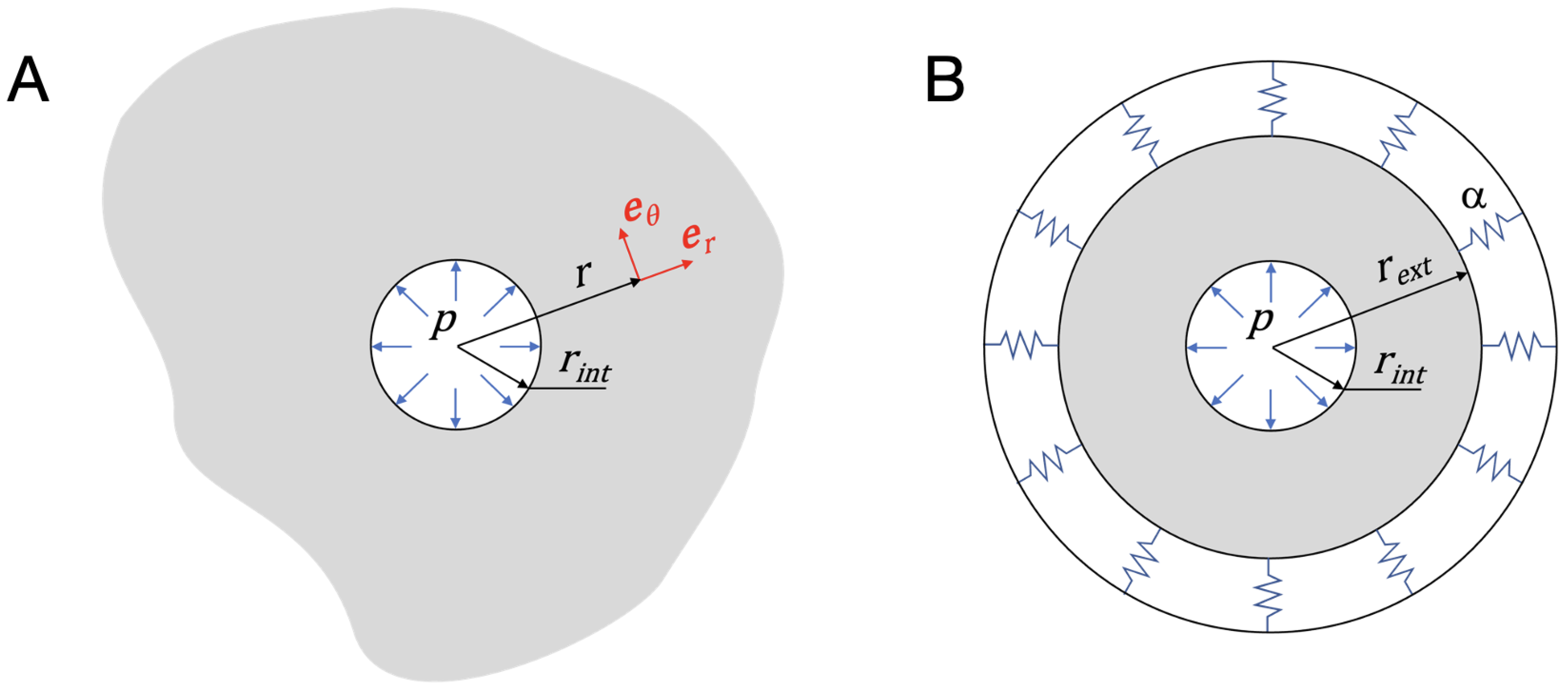
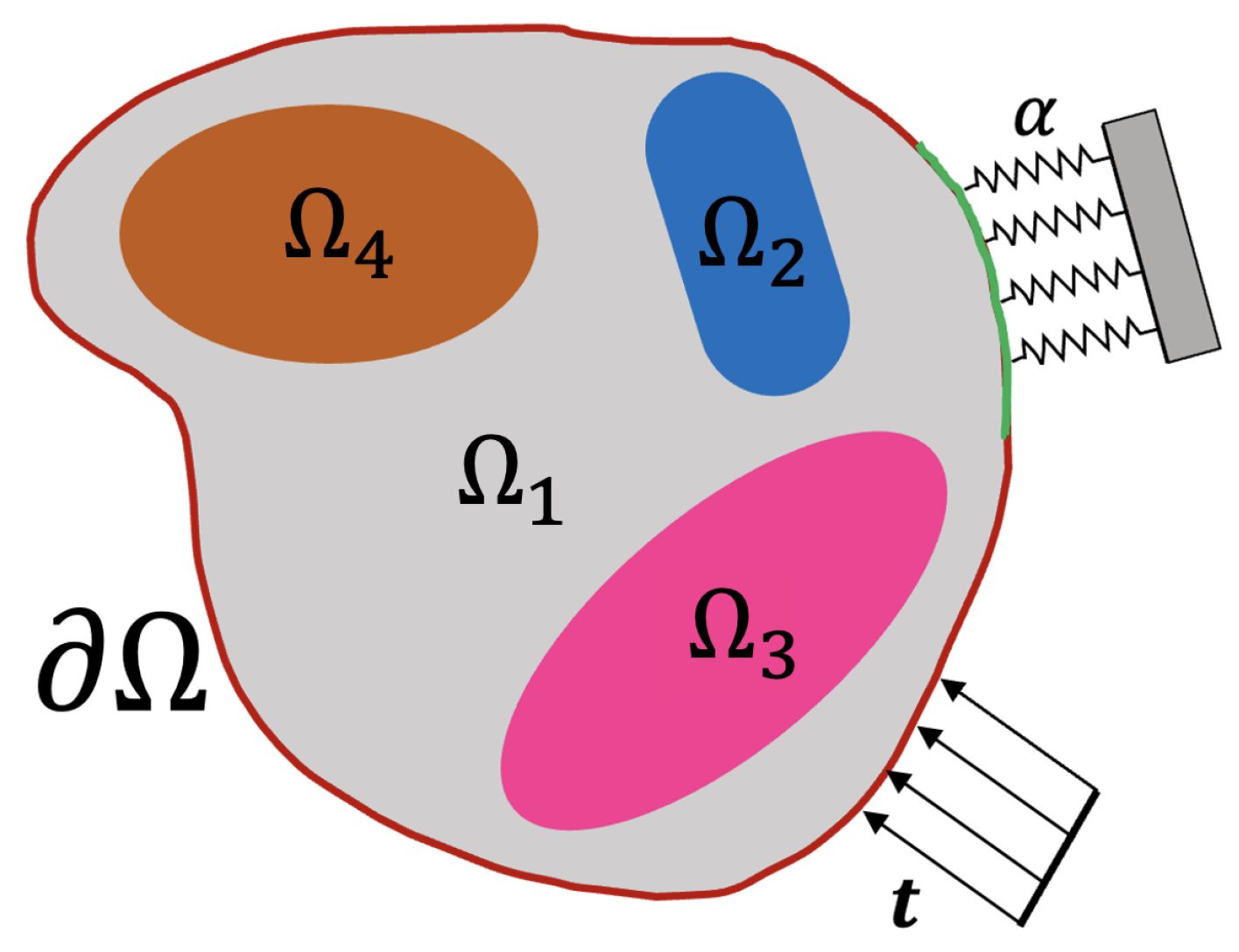
2.1. Problem Statement
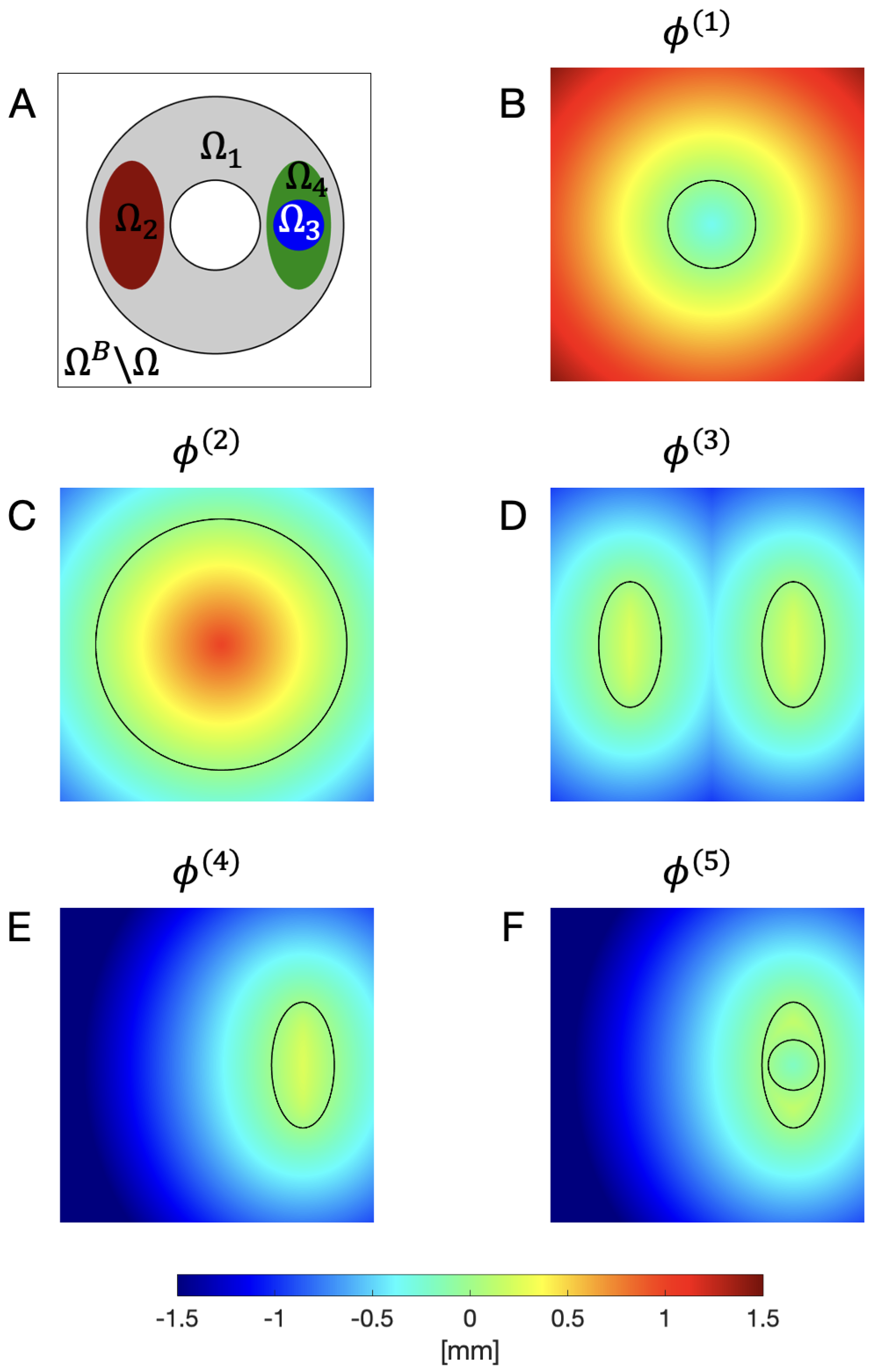
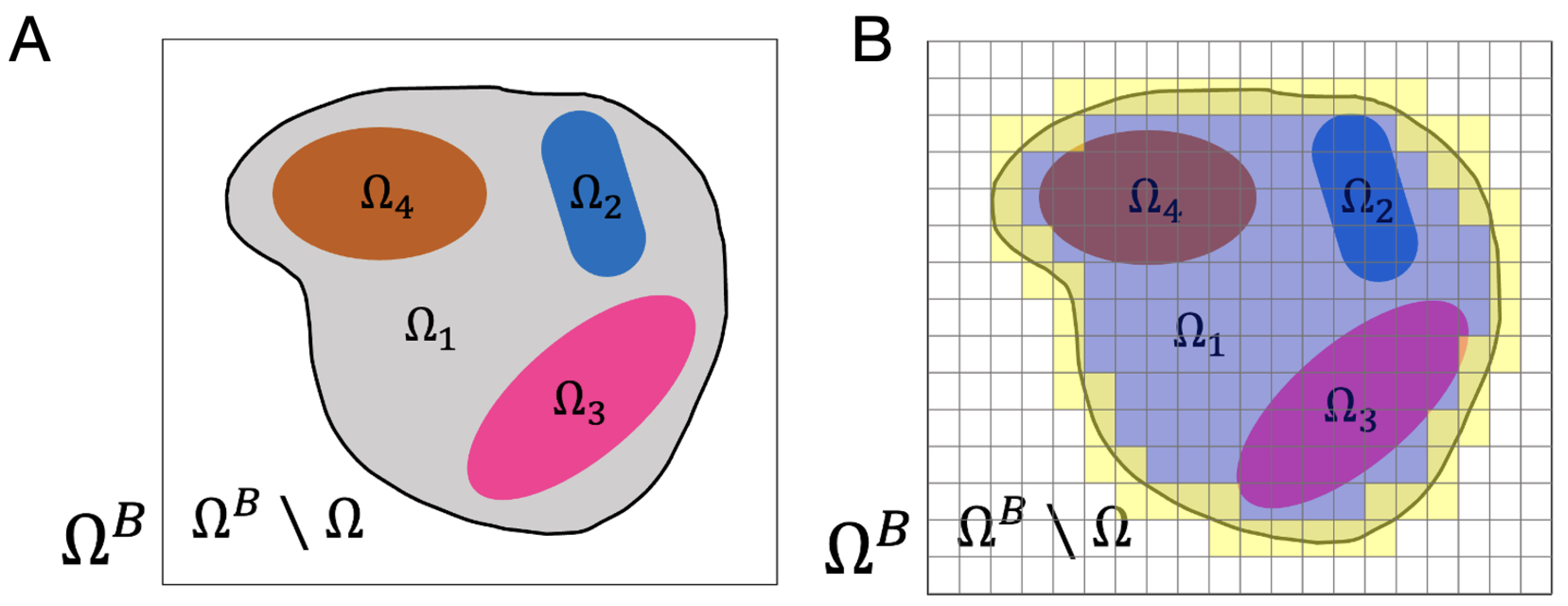
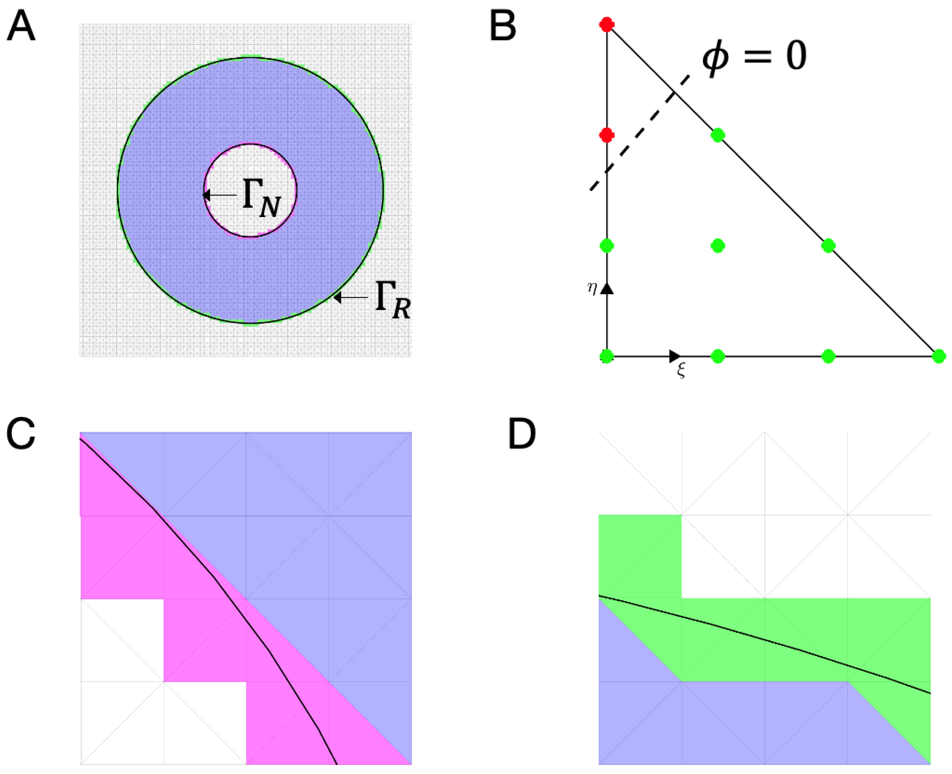
2.2. Level Set Description of the Domain and Subdomains
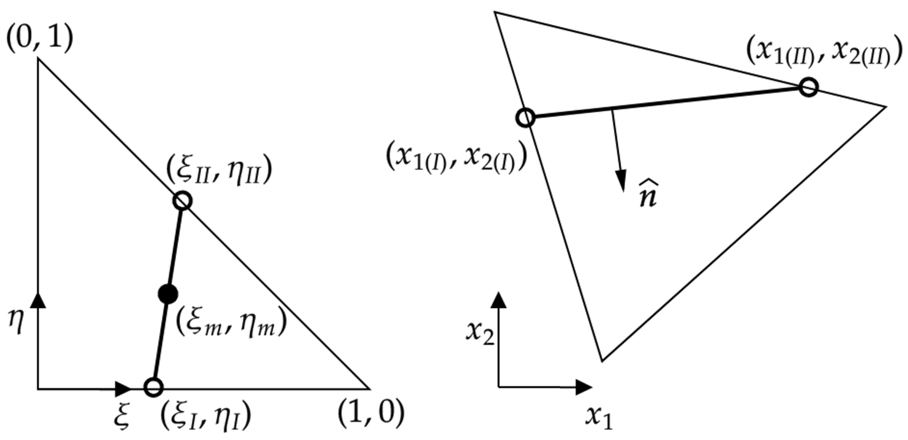
2.3. Discretization of the Level Set Functions in a Background Mesh
2.4. Unfitted Approach: Solving the Problem in the Background Mesh
2.5. Validating the Methodolgy
3. Results
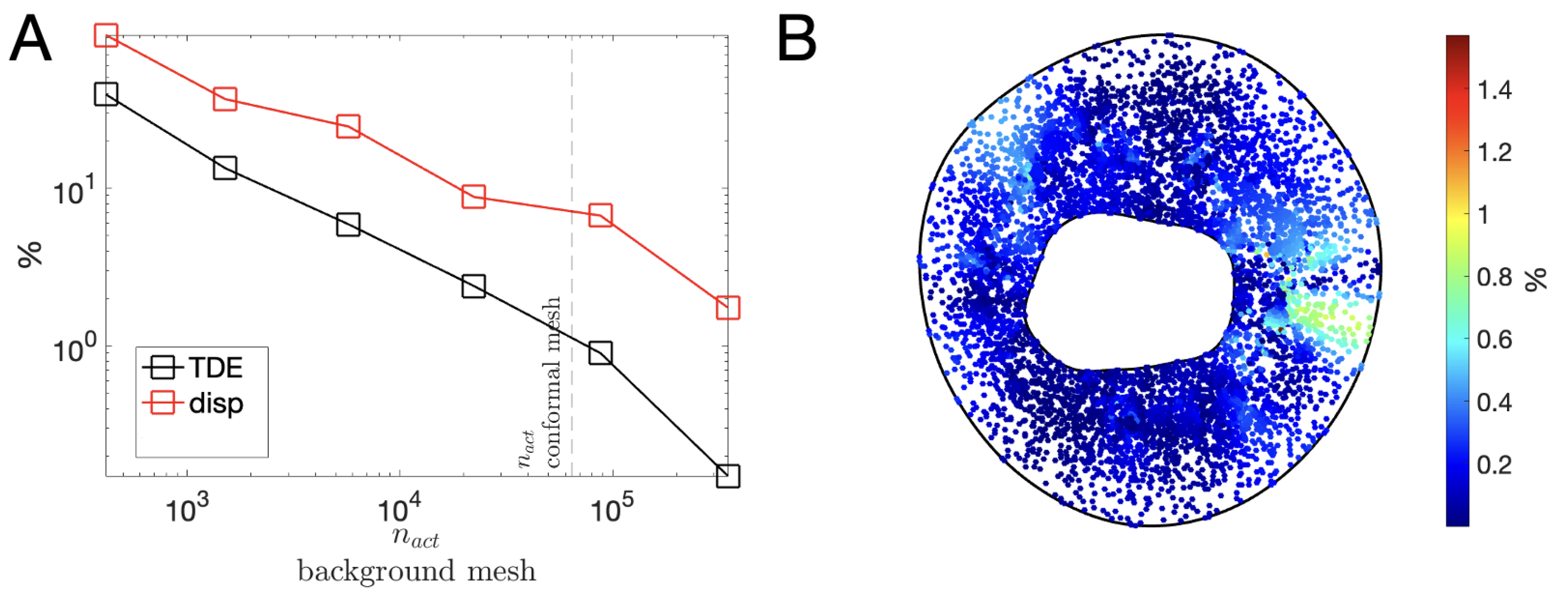
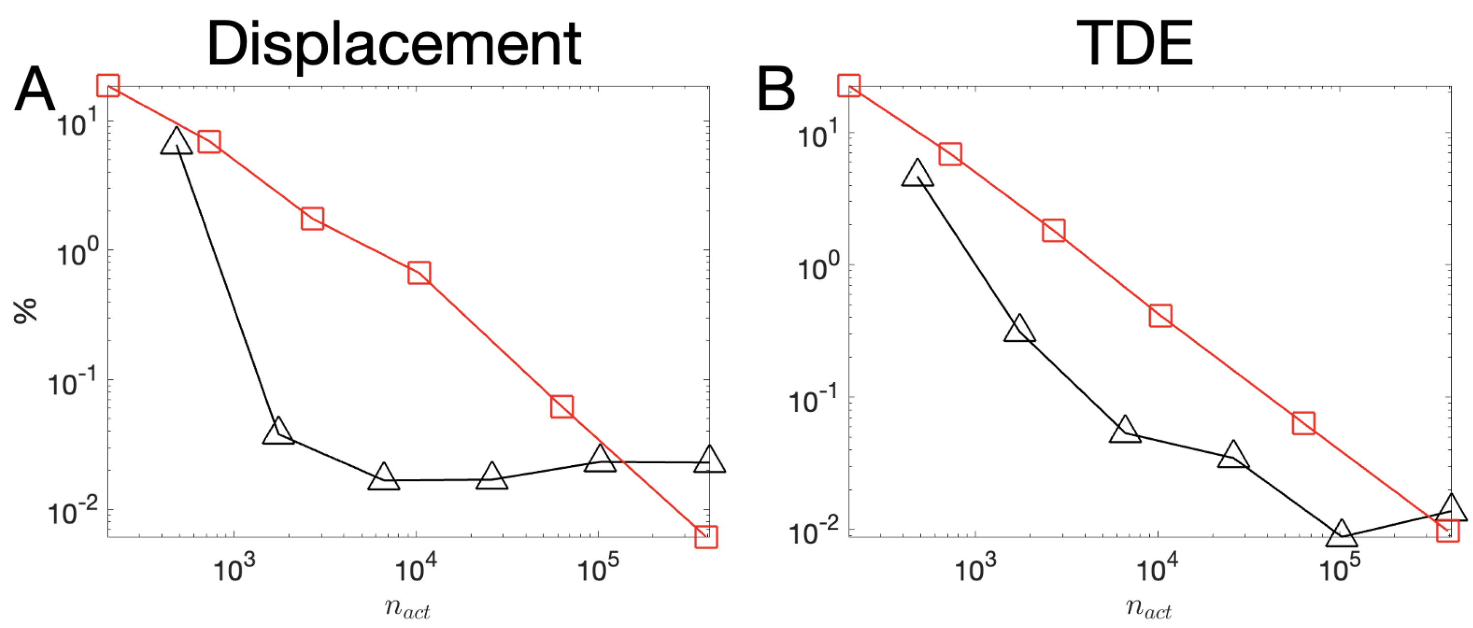
3.1. Covergence Analysis
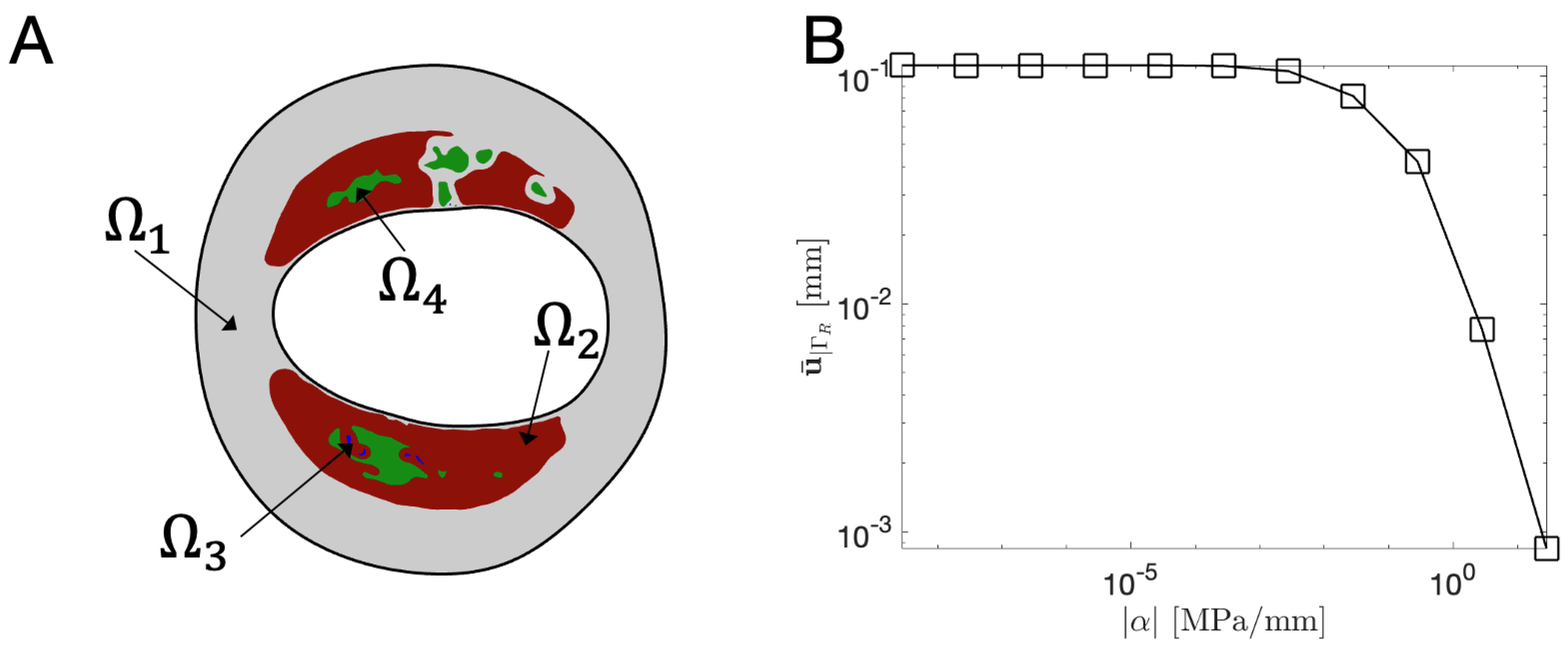
3.2. Elastic Bed Coeficient : Sensitivity Analysis
3.3. Characteristic Length h of the Background Mesh : Sensitivity Analysis
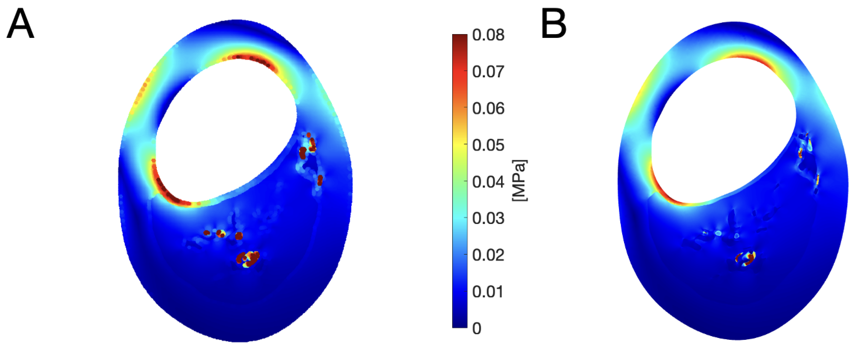
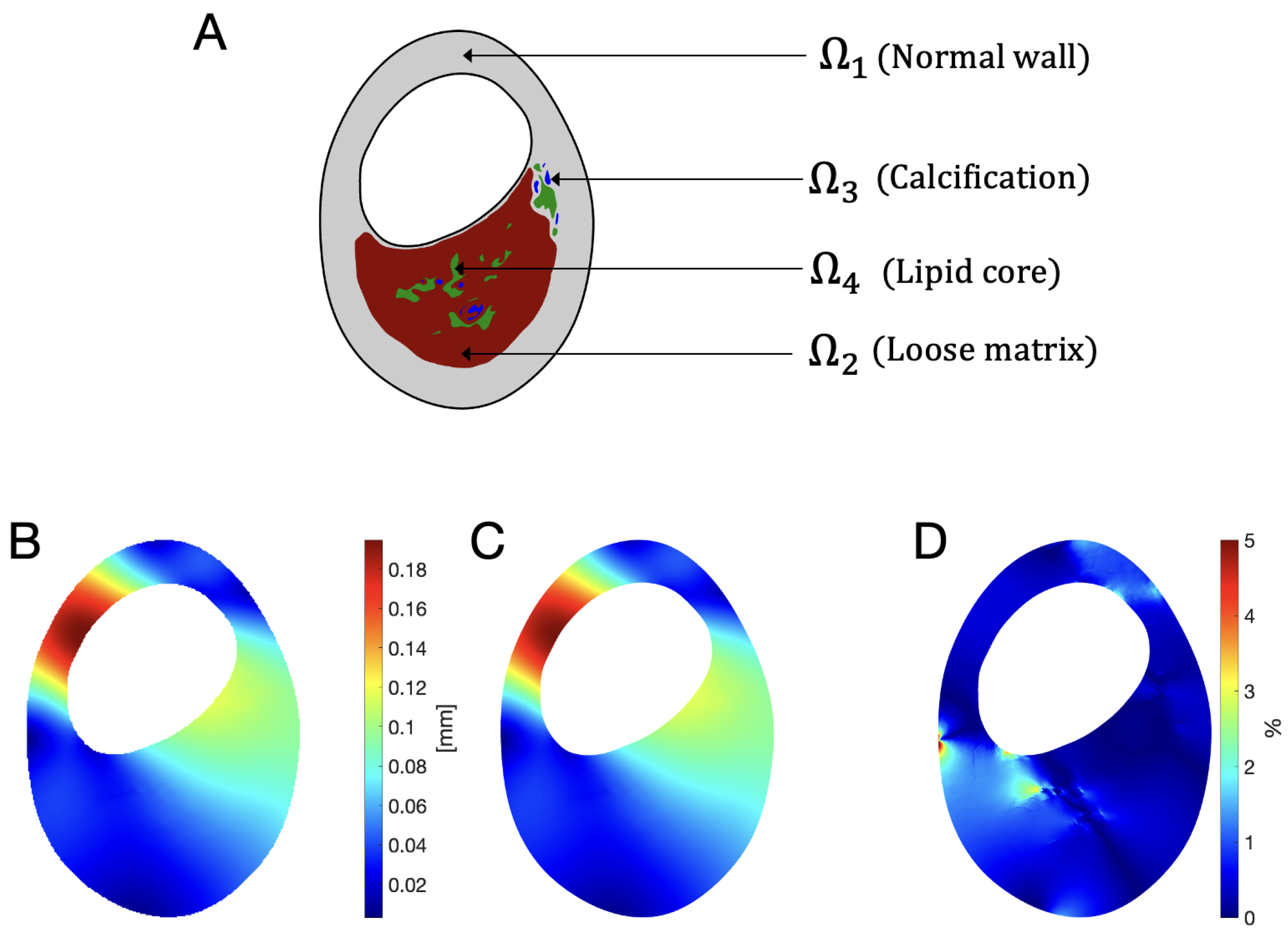
3.4. Realistic Immersed Boundary Robin-Based approach
4. Discussion
Author Contributions
Funding
Acknowledgments
Conflicts of Interest
Abbreviations
| BC | Boundary conditions |
| FE | Finite element |
| IB | Immersed Boundary |
| TDE | Total Deformation Energy |
References
- World Health Statistics 2020: Monitoring Health for the SDGs, Sustainable Development Goals. Available online: https://www.who.int/publications/i/item/9789240005105 (accessed on 20 September 2022).
- The Top 10 Causes of Death. Available online: https://www.who.int/news-room/fact-sheets/detail/the-top-10-causes-of-death (accessed on 20 September 2022).
- Thygesen, K.; Alpert, J.S.; White, H.D. Universal Definition of Myocardial Infarction. Circulation 2007, 116, 2634–2653. [Google Scholar] [CrossRef] [PubMed]
- Goyal, A.; Zeltser, R. Unstable Angina. Available online: https://www.ncbi.nlm.nih.gov/books/NBK442000/ (accessed on 27 September 2022).
- Holzapfel, G.A.; Mulvihill, J.J.; Cunnane, E.M.; Walsh, M.T. Computational approaches for analyzing the mechanics of atherosclerotic plaques: A review. J. Biomech. 2014, 47, 859–869. [Google Scholar] [CrossRef]
- Leiner, T.; Gerretsen, S.; Botnar, R.; Lutgens, E.; Cappendijk, V.; Kooi, E.; van Engelshoven, J. Magnetic resonance imaging of atherosclerosis. Eur. Radiol. 2005, 15, 1087–1099. [Google Scholar] [CrossRef]
- Corti, R.; Fuster, V. Imaging of atherosclerosis: Magnetic resonance imaging. Eur. Heart J. 2011, 32, 1709–1719. [Google Scholar] [CrossRef] [PubMed] [Green Version]
- Ostrom, M.P.; Gopal, A.; Ahmadi, N.; Nasir, K.; Yang, E.; Kakadiaris, I.; Flores, F.; Mao, S.S.; Budoff, M.J. Mortality Incidence and the Severity of Coronary Atherosclerosis Assessed by Computed Tomography Angiography. J. Am. Coll. Cardiol. 2008, 52, 1335–1343. [Google Scholar] [CrossRef] [Green Version]
- Achenbach, S.; Raggi, P. Imaging of coronary atherosclerosis by computed tomography. Eur. Heart J. 2010, 31, 1442–1448. [Google Scholar] [CrossRef] [Green Version]
- Yabushita, H.; Bouma, B.E.; Houser, S.L.; Aretz, H.T.; Jang, I.K.; Schlendorf, K.H.; Kauffman, C.R.; Shishkov, M.; Kang, D.H.; Halpern, E.F.; et al. Characterization of Human Atherosclerosis by Optical Coherence Tomography. Circulation 2002, 106, 1640–1645. [Google Scholar] [CrossRef] [PubMed]
- Araki, M.; Park, S.J.; Dauerman, H.L.; Uemura, S.; Kim, J.S.; Mario, C.D.; Johnson, T.W.; Guagliumi, G.; Kastrati, A.; Joner, M.; et al. Optical coherence tomography in coronary atherosclerosis assessment and intervention. Nat. Rev. Cardiol. 2022, 19, 684–703. [Google Scholar] [CrossRef]
- Böse, D.; von Birgelen, C.; Erbel, R. Intravascular Ultrasound for the Evaluation of Therapies Targeting Coronary Atherosclerosis. J. Am. Coll. Cardiol. 2007, 49, 925–932. [Google Scholar] [CrossRef] [Green Version]
- Garcia-Garcia, H.M.; Costa, M.A.; Serruys, P.W. Imaging of coronary atherosclerosis: Intravascular ultrasound. Eur. Heart J. 2010, 31, 2456–2469. [Google Scholar] [CrossRef]
- Akyildiz, A.C.; Speelman, L.; Nieuwstadt, H.A.; van Brummelen, H.; Virmani, R.; van der Lugt, A.; van der Steen, A.F.; Wentzel, J.J.; Gijsen, F.J. The effects of plaque morphology and material properties on peak cap stress in human coronary arteries. Comput. Methods Biomech. Biomed. Eng. 2016, 19, 771–779. [Google Scholar] [CrossRef]
- Kok, A.M.; van der Lugt, A.; Verhagen, H.J.; van der Steen, A.F.; Wentzel, J.J.; Gijsen, F.J. Model-based cap thickness and peak cap stress prediction for carotid MRI. J. Biomech. 2017, 60, 175–180. [Google Scholar] [CrossRef]
- Li, Z.Y.; Howarth, S.; Trivedi, R.A.; U-King-Im, J.M.; Graves, M.J.; Brown, A.; Wang, L.; Gillard, J.H. Stress analysis of carotid plaque rupture based on in vivo high resolution MRI. J. Biomech. 2006, 39, 2611–2622. [Google Scholar] [CrossRef]
- Sadat, U.; Teng, Z.; Young, V.; Graves, M.; Gaunt, M.; Gillard, J. High-resolution Magnetic Resonance Imaging-based Biomechanical Stress Analysis of Carotid Atheroma: A Comparison of Single Transient Ischaemic Attack, Recurrent Transient Ischaemic Attacks, Non-disabling Stroke and Asymptomatic Patient Groups. Eur. J. Vasc. Endovasc. Surg. 2011, 41, 83–90. [Google Scholar] [CrossRef] [Green Version]
- Gijsen, F.J.; Nieuwstadt, H.A.; Wentzel, J.J.; Verhagen, H.J.; van der Lugt, A.; van der Steen, A.F. Carotid Plaque Morphological Classification Compared With Biomechanical Cap Stress. Stroke 2015, 46, 2124–2128. [Google Scholar] [CrossRef] [Green Version]
- Nieuwstadt, H.A.; Kassar, Z.A.M.; van der Lugt, A.; Breeuwer, M.; van der Steen, A.F.W.; Wentzel, J.J.; Gijsen, F.J.H. A Computer-Simulation Study on the Effects of MRI Voxel Dimensions on Carotid Plaque Lipid-Core and Fibrous Cap Segmentation and Stress Modeling. PLoS ONE 2015, 10, e0123031. [Google Scholar] [CrossRef] [Green Version]
- Akyildiz, A.C.; Speelman, L.; van Brummelen, H.; Gutiérrez, M.A.; Virmani, R.; van der Lugt, A.; van der Steen, A.F.; Wentzel, J.J.; Gijsen, F.J. Effects of intima stiffness and plaque morphology on peak cap stress. BioMed. Eng. Online 2011, 10, 25. [Google Scholar] [CrossRef] [Green Version]
- Sadat, U.; Teng, Z.; Gillard, J.H. Biomechanical structural stresses of atherosclerotic plaques. Expert Rev. Cardiovasc. Ther. 2010, 8, 1469–1481. [Google Scholar] [CrossRef]
- Teng, Z.; Zhang, Y.; Huang, Y.; Feng, J.; Yuan, J.; Lu, Q.; Sutcliffe, M.P.; Brown, A.J.; Jing, Z.; Gillard, J.H. Material properties of components in human carotid atherosclerotic plaques: A uniaxial extension study. Acta Biomater. 2014, 10, 5055–5063. [Google Scholar] [CrossRef] [Green Version]
- Ebenstein, D.M.; Coughlin, D.; Chapman, J.; Li, C.; Pruitt, L.A. Nanomechanical properties of calcification, fibrous tissue, and hematoma from atherosclerotic plaques. J. Biomed. Mater. Res. Part A 2009, 91A, 1028–1037. [Google Scholar] [CrossRef]
- Milzi, A.; Lemma, E.D.; Dettori, R.; Burgmaier, K.; Marx, N.; Reith, S.; Burgmaier, M. Coronary plaque composition influences biomechanical stress and predicts plaque rupture in a morpho-mechanic OCT analysis. eLife 2021, 10, e64020. [Google Scholar] [CrossRef] [PubMed]
- Neumann, E.E.; Young, M.; Erdemir, A. A pragmatic approach to understand peripheral artery lumen surface stiffness due to plaque heterogeneity. Comput. Methods Biomech. Biomed. Eng. 2019, 22, 396–408. [Google Scholar] [CrossRef] [PubMed]
- Noble, C.; Carlson, K.D.; Neumann, E.; Lewis, B.; Dragomir-Daescu, D.; Lerman, A.; Erdemir, A.; Young, M.D. Finite element analysis in clinical patients with atherosclerosis. J. Mech. Behav. Biomed. Mater. 2022, 125, 104927. [Google Scholar] [CrossRef]
- Costopoulos, C.; Huang, Y.; Brown, A.J.; Calvert, P.A.; Hoole, S.P.; West, N.E.; Gillard, J.H.; Teng, Z.; Bennett, M.R. Plaque Rupture in Coronary Atherosclerosis Is Associated With Increased Plaque Structural Stress. JACC 2017, 10, 1472–1483. [Google Scholar] [CrossRef]
- Teng, Z.; Brown, A.J.; Calvert, P.A.; Parker, R.A.; Obaid, D.R.; Huang, Y.; Hoole, S.P.; West, N.E.; Gillard, J.H.; Bennett, M.R. Coronary Plaque Structural Stress Is Associated with Plaque Composition and Subtype and Higher in Acute Coronary Syndrome. Circulation 2014, 7, 461–470. [Google Scholar] [CrossRef] [Green Version]
- Madani, A.; Bakhaty, A.; Kim, J.; Mubarak, Y.; Mofrad, M.R.K. Bridging Finite Element and Machine Learning Modeling: Stress Prediction of Arterial Walls in Atherosclerosis. J. Biomech. Eng. 2019, 141, 84502. [Google Scholar] [CrossRef]
- Akyildiz, A.C.; Hansen, H.H.G.; Nieuwstadt, H.A.; Speelman, L.; Korte, C.L.D.; van der Steen, A.F.W.; Gijsen, F.J.H. A Framework for Local Mechanical Characterization of Atherosclerotic Plaques: Combination of Ultrasound Displacement Imaging and Inverse Finite Element Analysis. Ann. Biomed. Eng. 2016, 44, 968–979. [Google Scholar] [CrossRef] [Green Version]
- Akyildiz, A.C.; Speelman, L.; Velzen, B.V.; Stevens, R.R.; Steen, A.F.V.D.; Huberts, W.; Gijsen, F.J. Intima heterogeneity in stress assessment of atherosclerotic plaques. Interface Focus 2018, 8, 20170008. [Google Scholar] [CrossRef] [PubMed] [Green Version]
- Ohayon, J.; Gharib, A.M.; Garcia, A.; Heroux, J.; Yazdani, S.K.; Malvè, M.; Tracqui, P.; Martinez, M.A.; Doblare, M.; Finet, G.; et al. Is arterial wall-strain stiffening an additional process responsible for atherosclerosis in coronary bifurcations: An in vivo study based on dynamic CT and MRI. Am. J. Physiol. Heart Circ. Physiol. 2011, 301, H1097–H1106. [Google Scholar] [CrossRef] [PubMed] [Green Version]
- Morlacchi, S.; Pennati, G.; Petrini, L.; Dubini, G.; Migliavacca, F. Influence of plaque calcifications on coronary stent fracture: A numerical fatigue life analysis including cardiac wall movement. J. Biomech. 2014, 47, 899–907. [Google Scholar] [CrossRef]
- Peskin, C.S. The immersed boundary method. Acta Numer. 2002, 11, 479–517. [Google Scholar] [CrossRef] [Green Version]
- Aleksandrov, M.; Zlatanova, S.; Heslop, D.J. Voxelisation Algorithms and Data Structures: A Review. Sensors 2021, 21, 8241. [Google Scholar] [CrossRef] [PubMed]
- Tsai, A.; Yezzi, A.; Wells, W.; Tempany, C.; Tucker, D.; Fan, A.; Grimson, W.; Willsky, A. A shape-based approach to the segmentation of medical imagery using level sets. IEEE Trans. Med. Imaging 2003, 22, 137–154. [Google Scholar] [CrossRef] [Green Version]
- Ramesh, K.; Kumar, G.; Swapna, K.; Datta, D.; Rajest, S. A Review of Medical Image Segmentation Algorithms. EAI Endorsed Trans. Pervasive Health Technol. 2018, 7, e6. [Google Scholar] [CrossRef]
- Liu, X.; Song, L.; Liu, S.; Zhang, Y. A Review of Deep-Learning-Based Medical Image Segmentation Methods. Sustainability 2021, 13, 1224. [Google Scholar] [CrossRef]
- Taghanaki, S.A.; Abhishek, K.; Cohen, J.P.; Cohen-Adad, J.; Hamarneh, G. Deep semantic segmentation of natural and medical images: A review. Artif. Intell. Rev. 2021, 54, 137–178. [Google Scholar] [CrossRef]
- Quarteroni, A. Numerical Models for Differential Problems; Springer: Milan, Italy, 2014. [Google Scholar] [CrossRef]
- Gomes, J.; Faugeras, O. Reconciling Distance Functions and Level Sets. J. Vis. Commun. Image Represent. 2000, 11, 209–223. [Google Scholar] [CrossRef] [Green Version]
- Osher, S.; Fedkiw, R. Signed Distance Functions; Springer: Berlin/Heidelberg, Germany, 2003; pp. 17–22. [Google Scholar] [CrossRef]
- Zlotnik, S.; Díez, P. Hierarchical X-FEM for n-phase flow. Comput. Methods Appl. Mech. Eng. 2009, 198, 2329–2338. [Google Scholar] [CrossRef] [Green Version]
- Bayareh, M.; Mortazavi, S. Equilibrium Position of a Buoyant Drop in Couette and Poiseuille Flows at Finite Reynolds Numbers. J. Mech. 2012, 29, 53–58. [Google Scholar] [CrossRef]
- Silvester, P. Symmetric Quadrature Formulae for Simplexes. Math. Comput. 1970, 24, 95. [Google Scholar] [CrossRef]
- Mal, A.K.; Singh, S.J. Deformation of Elastic Solids; Prentice-Hall: Hoboken, NJ, USA, 1990. [Google Scholar]


| Condition | Classification |
|---|---|
| and | |
| and and | |
| and and and | |
| and and and and | |
| and and |
| E (MPa) | (MPa/mm) | (mm) | (mm) | |
|---|---|---|---|---|
| 4 |
| Subdomain | Material | E [MPa] | Ref. | |
|---|---|---|---|---|
| Normal vessel-wall | [22] | |||
| Loose matrix | [22] | |||
| Calcification | [23] | |||
| Lipid core | [22] |
| Mesh # | Diff. for TDE | max Diff. for Displacement Magnitude | |
|---|---|---|---|
| 1 | 414 | % | % |
| 2 | 1507 | % | % |
| 3 | 5734 | % | % |
| 4 | % | % | |
| 5 | % | % | |
| 6 | % | % |
| Active Elements | (MPa/mm) | ||
|---|---|---|---|
| 42,397 | 83,378 | ||
| 47,505 | 94,210 |
Disclaimer/Publisher’s Note: The statements, opinions and data contained in all publications are solely those of the individual author(s) and contributor(s) and not of MDPI and/or the editor(s). MDPI and/or the editor(s) disclaim responsibility for any injury to people or property resulting from any ideas, methods, instructions or products referred to in the content. |
© 2023 by the authors. Licensee MDPI, Basel, Switzerland. This article is an open access article distributed under the terms and conditions of the Creative Commons Attribution (CC BY) license (https://creativecommons.org/licenses/by/4.0/).
Share and Cite
Gahima, S.; Díez, P.; Stefanati, M.; Rodríguez Matas, J.F.; García-González, A. An Unfitted Method with Elastic Bed Boundary Conditions for the Analysis of Heterogeneous Arterial Sections. Mathematics 2023, 11, 1748. https://doi.org/10.3390/math11071748
Gahima S, Díez P, Stefanati M, Rodríguez Matas JF, García-González A. An Unfitted Method with Elastic Bed Boundary Conditions for the Analysis of Heterogeneous Arterial Sections. Mathematics. 2023; 11(7):1748. https://doi.org/10.3390/math11071748
Chicago/Turabian StyleGahima, Stephan, Pedro Díez, Marco Stefanati, José Félix Rodríguez Matas, and Alberto García-González. 2023. "An Unfitted Method with Elastic Bed Boundary Conditions for the Analysis of Heterogeneous Arterial Sections" Mathematics 11, no. 7: 1748. https://doi.org/10.3390/math11071748
APA StyleGahima, S., Díez, P., Stefanati, M., Rodríguez Matas, J. F., & García-González, A. (2023). An Unfitted Method with Elastic Bed Boundary Conditions for the Analysis of Heterogeneous Arterial Sections. Mathematics, 11(7), 1748. https://doi.org/10.3390/math11071748