Study on Queue Length in the Whole Process of a Traffic Accident in an Extra-Long Tunnel

Abstract

To investigate traffic accident patterns in undersea tunnels and quantify the relationship among various factors and traffic accidents in undersea tunnels, we analyzed the rules of evolution during the entire process of vehicle congestion queuing. Additionally, we built a maximum queue-length estimation model based on shock-wave theory and a whole-process queue-length estimation model based on real-time data input. The results demonstrate that the model is most precise when the data are not smoothed and the time interval is 30 s. The maximum accuracy of the model is not improved by data smoothing processing, but it is substantially improved when the time interval is between 5 and 15 s. Various movable window lengths have no discernible effect on the results. Maximum queue-length estimation model accuracy is 92.34%, while real-time whole-process queue-length estimation model accuracy is 83.50%. The accuracy of the proposed model is greater than that of the input–output model, indicating that the proposed model can support timely and reasonable control measures.

1. Introduction

Extra-long tunnels have more complex traffic environment features than regular sections, and their internal driving safety and stability are poor, making tunnels a highly accident-prone stretch. When management actions for abrupt traffic incidents are delayed, congestion spreads quickly, and the space–time impact of congestion becomes more severe. Queue length is an important metric that reflects the degree of tunnel congestion and serves as the data foundation for conducting tunnel traffic control techniques. Traditional queue-length estimation research relies heavily on traffic flow data gathered by fixed-point detectors such as inductive loops (inductive loop detectors). However, owing to the reinforced concrete structure, the coverage of the fixed detectors in extra-long tunnels is limited and easily damaged, and the weak or nonexistent positioning signal causes GPS data to fail. Consequently, utilizing the effective data available in the tunnel to accurately grasp the evolution law of accident congestion in extra-long tunnels and obtaining traffic flow parameters such as vehicle queue length in a timely manner will improve the management and control efficiency of extra-long tunnels following traffic accidents and reduce the impact of tunnel traffic accidents on traffic flow operation.

Currently, most queue-length estimation research is focused on signalized intersections [1,2,3,4] and highways [5,6]. Traffic congestion is likely to develop following an accident due to the tunnel’s structural characteristics. If it is not evacuated in a timely way, queueing occurs, affecting the road’s normal traffic efficiency. Owing to a dearth of structured traffic flow data throughout the accident process, there are few studies on queue length in the backdrop of the accident. Pan et al. [7] developed a traffic congestion evacuation decision model for highway tunnels that can predict traffic characteristics such as traffic congestion time and queue length following accidents at all levels of the tunnel. Huang [8] predicted the length of the vehicle queue using the traffic wave model and the traffic flow characteristics of highway tunnel accidents. Guang et al. [9] proposed an analytical method for measuring entrance ramp queue length and developed a simulation model for estimating queue length in various demand–capacity scenarios. Although these studies can predict vehicle queue lengths in accidents, they cannot estimate vehicle queue lengths in real time due to a lack of real-time traffic flow data in accidents. Compared to tunnels, urban road data sources are more abundant, and real-time traffic data [10] are utilized more frequently. Existing research data include GPS data [11,12,13], license plate recognition data [14,15,16], mobile sensors [17], trajectory data [18], video data [19], etc. Furthermore, with the advancement of intelligent networking technology, reports in the literature [20,21,22,23,24,25,26] provide new data concepts for the study of real-time queue-length estimation.

Most of the research on queue length of vehicles in traffic accidents focuses on queue-length estimation, but lacking appropriate data; this paper examines the evolution law of vehicle congestion queueing from generation to spread to dissipation following traffic accidents in extremely lengthy tunnels. The maximum queuing length model and the real-time estimation model of vehicle queuing length are proposed based on traffic flow shock-wave theory. The main contributions of this paper follow:

(1)

A video system was placed inside the lengthy tunnel; the information gathered from it is clear and trustworthy, and it is continuously arranged at a specific distance. As a result, the side-mounted video data were selected as the data source for the model analysis in this paper, which could provide data support for estimating queue length in real time.

(2)

Based on real-time data input, this paper analyzed the influence of forward and backward shock waves on vehicle queue length and revealed the process mechanism of the formation, spread, and dissipation of vehicle queue in the overall process of traffic accidents. There are relatively few studies that account for the evolution characteristics of vehicle queue length in the whole process of accidents.

(3)

According to [27,28,29,30,31], the length of the vehicle line in a particular section was calculated by estimating the difference between the number of vehicles entering and exiting the area through a given amount of time. To calculate the length of vehicles queuing in space, the vertical queue length was split by the density of vehicles. Since it is challenging to collect continuous traffic variables in a real-world traffic setting, the detector cleverly collects discrete values of traffic flow variables. In order to increase the precision of vehicle queuing estimation, the technique suggested in this paper was used to thoroughly investigate the congestion characteristics of traffic flow after accidents in tunnels.

2. Materials and Methods

2.1. Characteristics of Traffic Flow Parameters in the Entire Process of Traffic Accidents

Figure 1 depicts the spatial–temporal distribution diagram of the flow density velocity of the entire process, which was derived using a traffic accident that occurred in the Qingdao Jiaozhou Bay Long Submarine Tunnel on 1 May 2019 in the morning. Prior to 10:09 a.m., the flow in the tunnel fluctuated between roughly 2000 and 4000 veh/h, the density was less than 100 veh/km, and the speed was between 50 and 60 km/h. Following the accident, traffic on the accident section dropped to less than 2000 vehicles per hour, the density of the accident section increased to more than 200 vehicles per km, the speed on the accident section dropped to less than 10 km per hour, and the impact area of the congestion was close to 1200 m. The flow rate of the accident section rose abruptly from 1500 to 4000 veh/h after the accident was cleared, the density gradually decreased, the speed recovered from less than 10 km/h to more than 30 km/h, and the traffic capacity returned to normal. However, the flow rate quickly returned to zero, and a “vacuum belt” with a flow rate of zero (the dark depression in the figure) clearly emerged on the figure, lasting approximately 4 min. The “zero flow” phenomenon is associated with excess flow control following tunnel incidents. Because relevant management and control departments were unable to obtain dynamic change information of vehicle queues in the tunnel on-time and directly, they did not change the flow control measures after traffic resumed smooth operation in the tunnel following the accident, resulting in the waste of traffic capacity in the tunnel and exacerbating the travel time delay caused by the accident.

2.2. Analysis of the Evolutionary Process of Traffic-Accident Vehicle Queue Length

The extra-long tunnel’s traffic accident queue can be divided into three stages: queue generation, queue spread, and queue dissipation. In this paper, the analysis and research are conducted under the assumption that the vehicles involved in the traffic accident in the extra-long tunnel are towed away at the same time (there is no secondary clearing of the vehicles occupying the road), and that the control time after the accident is earlier than the accident’s end time.

2.2.1. Queue Generation

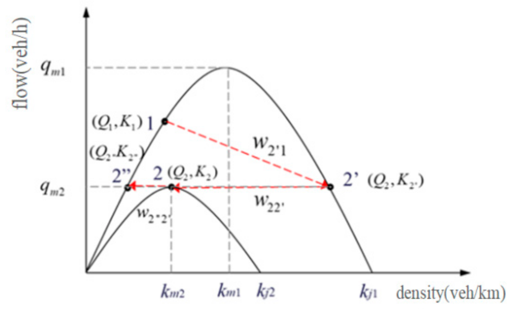
When an accident occurs, the traffic capacity of the accident section decreases sharply due to the accident vehicle occupying the road. The flow–density relationship of the accident section is shown in Figure 2. $q_{\mathrm{m}1}$ is the normal traffic capacity in tunnel; $k_{\mathrm{m}2}$ is the best density when the traffic capacity of the accident section in the tunnel is the largest; $k_{j1}$ is the blocking density of the accident section; $Q_i$ is the traffic flow under state $i$; $k_i$ is the density under state $i$; $w_{\mathit{ij}}$ is the shock wave generated between the traffic flow running state $i$ and state $j$, and $V_{w_{\mathit{ij}}}$ is the velocity of shock wave $w_{\mathit{ij}}$. State 1 is the unblocked state, state 2′ is the congested state, state 2 is the congested state, and state 2′′ is the unblocked state. At this time, the capacity of the accident section is reduced from $q_{\mathrm{m}1}$ to $q_{\mathrm{m}2}$.The traffic flow in the tunnel is shown in Figure 3.

If the traffic flow after the accident exceeds the remaining capacity of the accident section, the traffic flow changes from state 1 to state 2, the accident section forms a bottleneck, and vehicles that cannot pass in time begin to queue. The traffic flow state of the adjacent road segment upstream from the accident section changes from state 1 to state 2′. As depicted by the dashed line 1–2′ in Figure 2, the collision of traffic flow in distinct traffic states will produce a shock wave. As depicted in Figure 2 dotted line 2–2, shock waves will be generated between the accident section state 2 and the upstream state 2′, and between the accident section state 2 and the downstream state 2′′.

At this time, wave velocity $V_{w_{22\prime }}$ of shock wave $w_{22\prime }$ can be obtained because $Q_2=Q_{2^{\prime }},K_2<K_{2^{\prime }}$:

$$V_{w_{{22}^{\prime }}}=\frac{Q_2-Q_{2^{\prime }}}{K_2-K_{2^{\prime }}}=0$$

(1)

The velocity of shock wave $w_{{22}^{\prime }}$ is zero, and it will not propagate upstream or downstream. Similarly, the velocity of shock wave $w_{{22}^{″}}$ is also zero.

$Q_1>Q_{2^{\prime }},K_2<K_{2^{\prime }}$, therefore, wave velocity $V_{w_{2^{\prime }1}}$ of shock wave $w_{2^{\prime }1}$ is:

$$V_{w_{2^{\prime }1}}=\frac{Q_{2^{\prime }}-Q_1}{K_{2^{\prime }}-K_1}<0$$

(2)

When the wave velocity of shock wave $w_{2^{\prime }1}$ is less than zero, the shock wave propagates in the opposite direction of the traffic flow, that is, upstream. At this time, congestion occurs and vehicles begin to queue.

2.2.2. Queue Spread

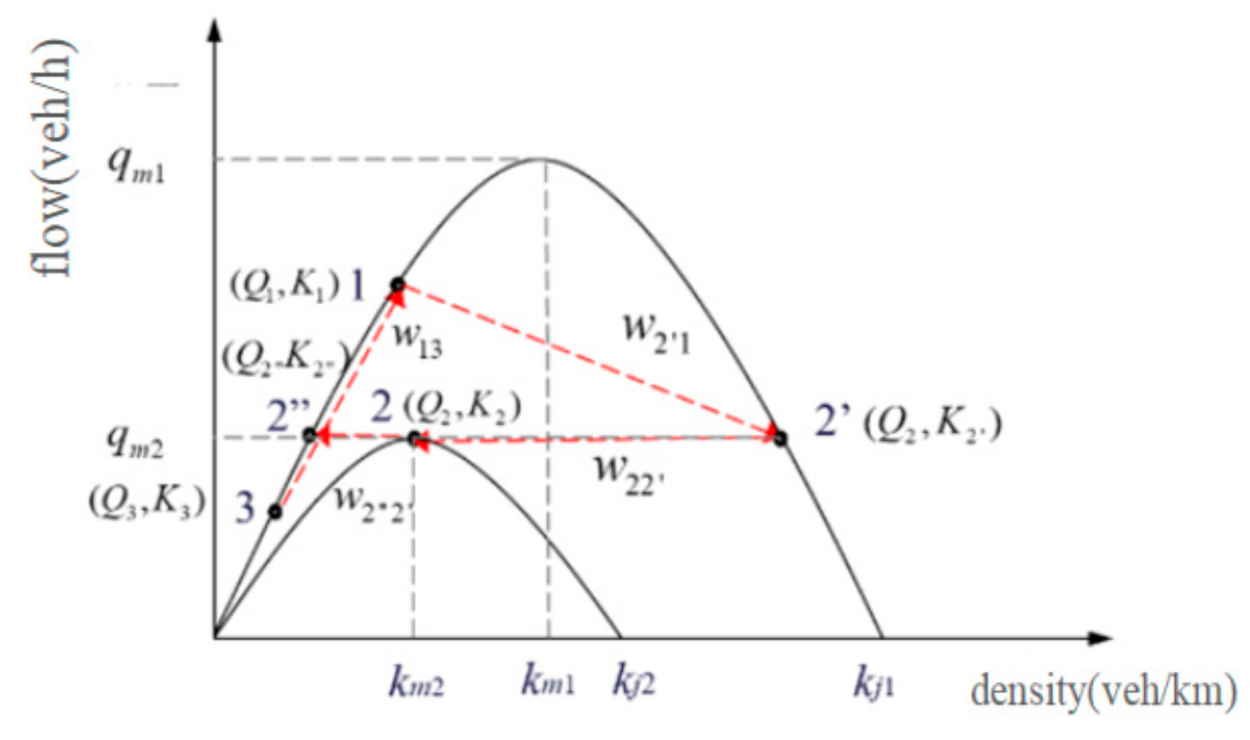
The flow control point begins to implement flow control after queuing (this paper assumes that the flow control point is located at the tunnel entrance). The volume of traffic entering the tunnel begins to decrease at this time. Figure 4 depicts the flow–density for each state in the tunnel.

The traffic flow operation status is shown in Figure 5. After the flow control is implemented, the traffic flow operation status from the accident section to the flow control point can be divided into five categories (the traffic flow status outside the flow control point is not considered in this paper), followed by the unblocked state 2’’, the traffic flow equal to the residual traffic capacity of the accident Section 2, the congestion queuing state 2 ‘, the normal operation state 1 before the accident, and state 3 after the flow control.

At this time, when the traffic flow of state 3 meets the traffic flow of state 1, shock wave $w_{13}$ is generated. $Q_3<Q_1,K_3<K_1$, therefore, wave velocity $V_{w_{13}}$ of shock wave $w_{13}$ is:

$$V_{w_{13}}=\frac{Q_3-Q_1}{K_3-K_1}>0$$

(3)

When the velocity of a shock wave is greater than zero, the shock wave propagates in the same direction as the traffic flow, i.e., without congestion downstream. At this time, the aggregation wave continues to propagate upstream, the traffic flow of state 1 gradually transitions to state 2′, and the length of the vehicle queue grows.

2.2.3. Queuing Dissipation

(1)

The traffic-flow running state when the traffic flow after control meets the queuing traffic flow.

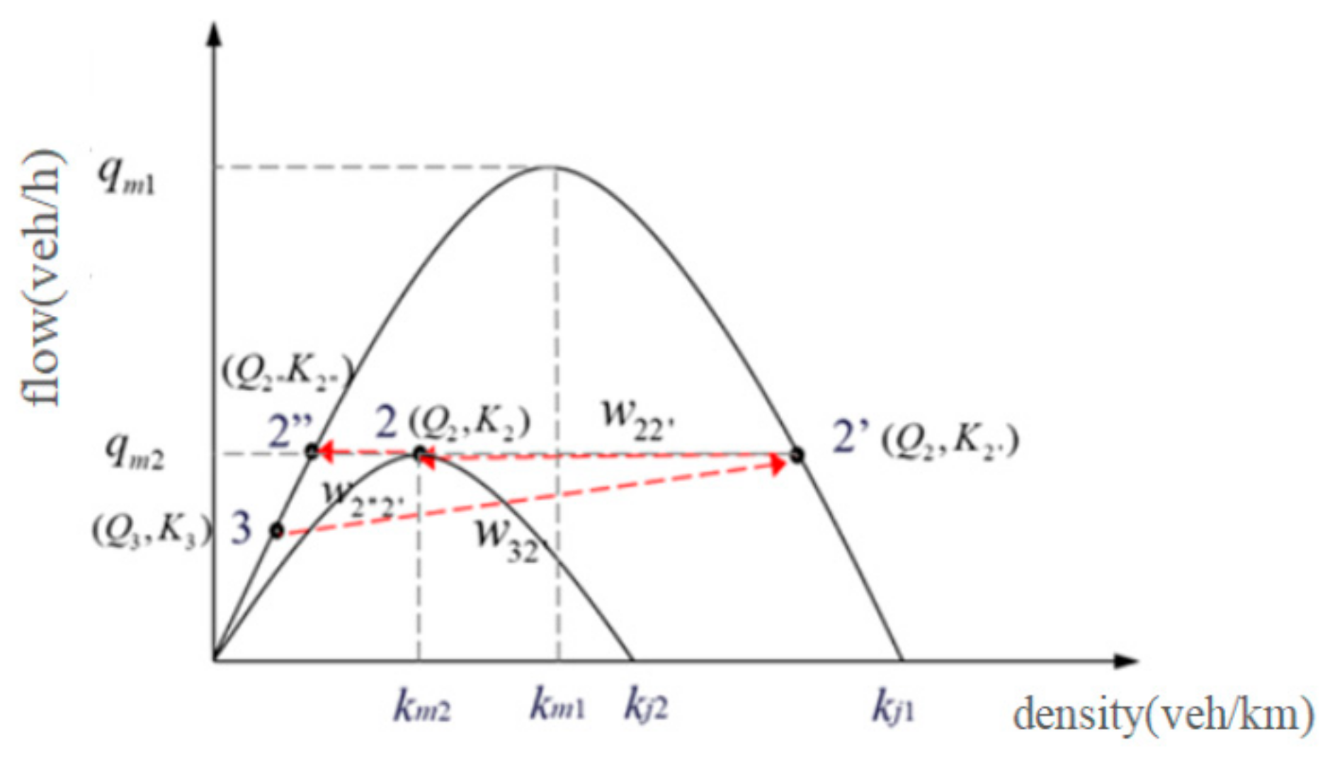
When the accumulation wave passes through all the vehicles in state 1, the flow–density of each state in the tunnel is shown in Figure 6, and the traffic flow condition is shown in Figure 7. The traffic flow from the accident section to the control point can be divided into four categories: state 2″, state 2, state 2′, and state 3. At this time, the state 3 traffic flow with its small flow and the state 2′ traffic flow in the congested queue meet to generate a shock wave, as shown in Figure 6 dotted line 3–2′.

At this time, shock wave $w_{{32}^{\prime }}$ will be generated when the traffic flow of state 3 meets the traffic flow of state 2′, $Q_3<Q_{2^{\prime }},K_3<K_{2^{\prime }}$, therefore, wave velocity $V_{w_{{32}^{\prime }}}$ of shock wave $w_{{32}^{\prime }}$ is:

$$V_{w_{{32}^{\prime }}}=\frac{Q_3-Q_{2^{\prime }}}{K_3-K_{2^{\prime }}}>0$$

(4)

The velocity of shock wave $V_{w_{{32}^{\prime }}}$ is greater than zero, which is a forward wave, and the queue length begins to decrease.

(2)

Traffic flow running state after accident clearance

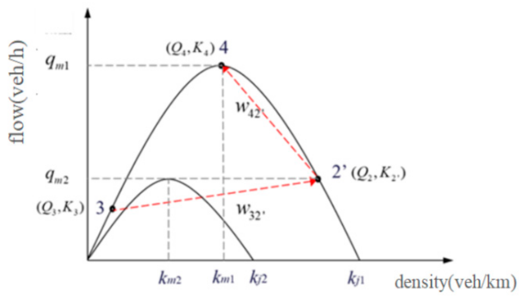
When the accident vehicle is cleared, the traffic capacity of the accident section returns to normal. At this time, the flow–density of each state is shown in Figure 8, and the traffic flow operation status is shown in Figure 9. The capacity of the accident section increases from $q_{\mathrm{m}2}$ to $q_{\mathrm{m}1}$, assuming that the traffic flow state of the accident section reaches saturation, the traffic flow running state from the accident section to the flow control point can be divided into three categories: state 4, state 2′, and state 3. The upstream queuing vehicles begin to gradually accelerate, so the accident section and the downstream section change from the original state 2 to state 4, and the state 2′ traffic flow changes to state 4, resulting in shock wave $w_{{42}^{\prime }}$, as shown in Figure 8 dotted line 2′–4.

At that time, wave velocity $V_{w_{2^{\prime }1}}$ of shock wave $w_{2^{\prime }1}$ is shown as slow because $Q_4>Q_{2^{\prime }},K_4<K_{2^{\prime }}$.

$$V_{w_{{42}^{\prime }}}=\frac{Q_4-Q_{2^{\prime }}}{K_4-K_{2^{\prime }}}<0$$

(5)

The wave velocity of shock wave $w_{{42}^{\prime }}$ is less than zero, indicating that shock wave $w_{{42}^{\prime }}$ is a backward wave, propagating in the opposite direction of the traffic flow until it meets shock wave $V_{w_{{32}^{\prime }}}$.

(3)

The running state of traffic flow when the traffic flow after control meets the saturated traffic flow.

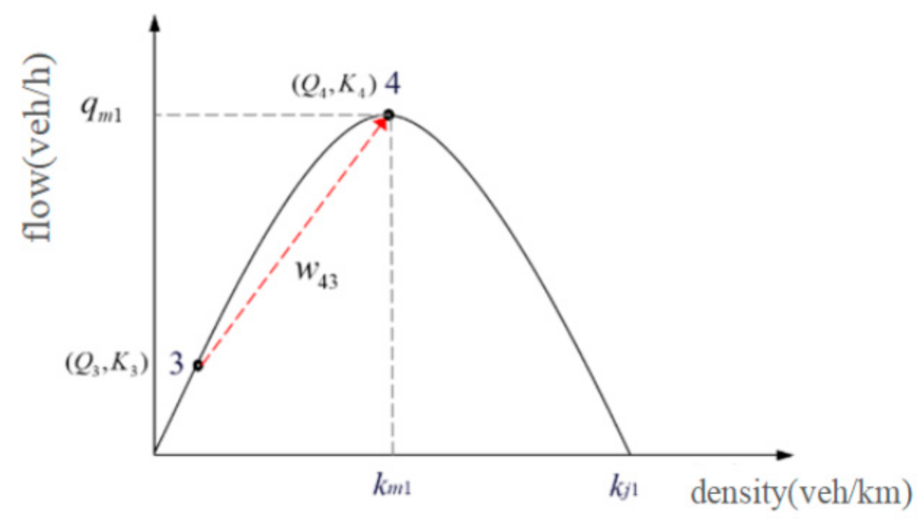
When shock wave $w_{{32}^{\prime }}$ encounters dissipated wave $w_{{42}^{\prime }}$, it means that the controlled state 3 traffic flow meets the saturated traffic flow of state 4, and the traffic flow–density of each state is shown in Figure 10; the traffic flow status is shown in Figure 11.

At that time, $Q_3<Q_{2^{\prime }},K_3<K_{2^{\prime }}$, therefore, wave velocity $V_{w_{{32}^{\prime }}}$ of shock wave $w_{{32}^{\prime }}$ is:

$$V_{w_{43}}=\frac{Q_4-Q_3}{K_4-K_3}>0$$

(6)

Therefore, if the wave velocity of shock wave $w_{43}$ is greater than zero, shock wave $w_{43}$ is a forward wave, spreading in the direction of vehicle flow, and the queue begins to dissipate until the vehicles at the end of the queue pass the accident section, and the queue dissipates.

2.3. Maximum Queue-Length Estimation Model

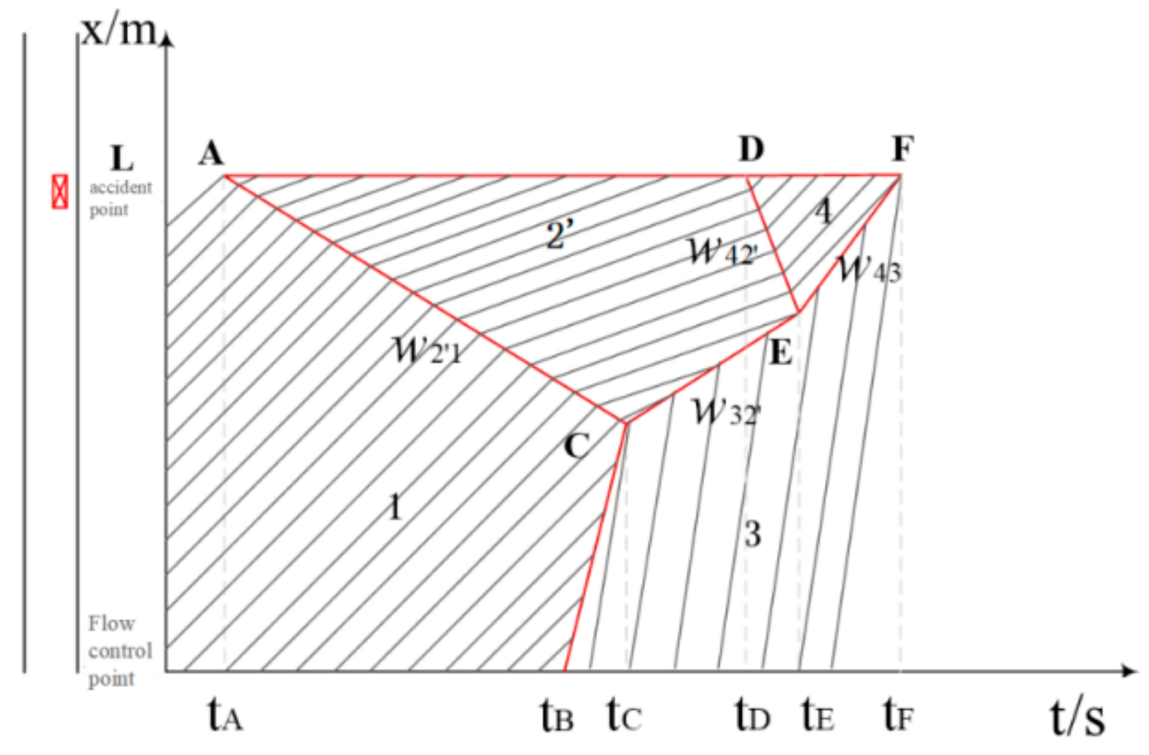
According to the shock-wave theory of traffic flow, the evolution process of vehicle queue length in traffic accidents and the change characteristics of flow, density, and speed in the whole process, the time–space operation trajectory diagram of vehicles is shown in Figure 12. The horizontal axis represents the time and the vertical axis represents the distance between the accident point and the flow control point near the tunnel entrance.

In the figure, $t_{\mathrm{A}}$ is the time of the accident; $t_{\mathsf{{\rm B}}}$ is the start time of flow control; $t_{\mathrm{C}}$ is the time when the controlled traffic flow meets the queuing traffic flow, that is, the time when the queuing length reaches the maximum; $t_{\mathrm{D}}$ is the end time of the accident; $t_{\mathrm{E}}$ represents the time when shock wave $w_{{32}^{\prime }}$ meets shock wave $w_{{42}^{\prime }}$; and $t_{\mathrm{F}}$ is the time that the maximum queue-length tail vehicle passes through the accident section.

The line AC can represent the propagation path of shock wave $w_{2^{\prime }1}$, generated when state 1 meets state 2′, that is, the path where the vehicle begins to queue. The line CE can represent the propagation path of shock wave $w_{{32}^{\prime }}$ generated when state 3 meets state 2′. Line DE represents the propagation path of shock wave $w_{2^{\prime }1}$ generated when state 2′ meets state 4. The line EF represents the propagation path of shock wave $w_{43}$ generated when state 3 meets state 4.

The calculation formula for time $t_{\mathrm{C}}$ when the controlled traffic flow meets the queuing traffic flow is as follows:

$$t_{\mathrm{C}}=t_{\mathrm{B}}+\frac{L-l_{\max }}{V_3}$$

(7)

Through geometric analysis of the vehicle time–space trajectory diagram, the following can be obtained:

$$l_{\max }=V_{w_{2^{\prime }1}}(t_{\mathrm{C}}-t_{\mathrm{A}})$$

(8)

The maximum queue length $l_{\max }$ can be obtained by combining Formulas (7) and (8).

$$l_{\max }=V_{w_{2^{\prime }1}}\frac{L+V_3(t_{\mathrm{B}}-t_{\mathrm{A}})}{V_3+V_{w_{2^{\prime }1}}}$$

(9)

According to Formulas (7) and (9), the time of maximum queue length $t_{\mathrm{C}}$ can be obtained. In addition, through the geometric analysis of the vehicle time–space trajectory diagram, the time $t_{\mathrm{E}}$ when the two dissipated waves meet, the time $t_{\mathrm{F}}$ when the tail vehicle passes the accident section, and the duration of the accident can be obtained. The calculation formula can be expressed as:

$$l_{\max }=V_{w_{{32}^{\prime }}}(t_{\mathrm{E}}-t_{\mathrm{C}})+V_{w_{{42}^{\prime }}}(t_{\mathrm{E}}-t_{\mathrm{D}})$$

(10)

$$t_{\mathrm{F}}=t_{\mathrm{E}}+\frac{(t_{\mathrm{E}}-t_{\mathrm{D}})V_{w_{{42}^{\prime }}}}{V_{w_{43}}}$$

(11)

$$t_{\max }=t_{\mathrm{A}}-t_{\mathrm{F}}$$

(12)

Through this analysis, the maximum queue-length calculation model with flow, density, speed, and distance between the accident location and the hole as variables can be constructed, as shown in Formula (13):

$$l_{\max }=(q_{\mathrm{u}}-q_{\mathrm{jam}})\left[L+v_{\mathrm{u}}(t_{\mathrm{B}}-t_{\mathrm{A}})\right]/(v_{\mathrm{u}}{k}_{\mathrm{u}}-v_{\mathrm{u}}{k}_{\mathrm{jam}}+q_{\mathrm{u}}-q_{\mathrm{jam}})$$

(13)

$$v_{\mathrm{u}}{k}_{\mathrm{u}}=q_{\mathrm{u}},\Delta v=t_{\mathrm{B}}-t_{\mathrm{A}}$$

(14)

The final $l_{\max }$ can be expressed as:

$$l_{\max }=(q_{\mathrm{u}}-q_{\mathrm{jam}})(L+v_{\mathrm{u}}\Delta \mathrm{t})/(2q_{\mathrm{u}}-v_{\mathrm{u}}{k}_{\mathrm{jam}}-q_{\mathrm{jam}})$$

(15)

In the formula, $l_{\max }$ is the maximum queue length; $L$ is the distance between the accident location and the tunnel entrance; $V_3$ is the vehicle speed after control; $q_{\mathrm{u}}$ is the upstream traffic volume in the tunnel; $v_{\mathrm{u}}$ is the upstream velocity in the tunnel; $k_{\mathrm{u}}$ is the upstream traffic density in the tunnel; $q_{\mathrm{jam}}$ is the residual traffic capacity of the accident section; $k_{\mathrm{jam}}$ is blocking density; $\Delta t$ is the control start time; and $t_{\max }$ is the duration of the accident impact.

2.4. Real-Time Estimation Model of Vehicle Queue Length in the Whole Process

The maximum queue-length estimation model can estimate the spatial range length affected by traffic accidents, but it cannot precisely estimate the real-time vehicle queue length based on the geometric analysis of vehicle time–space trajectory line under ideal conditions (constant vehicle arrival rate). In reality, the arrival of vehicles is random, and the parameters of traffic flow data fluctuate greatly, making it difficult to estimate an accurate value for the fixed wave velocity. In order to achieve an accurate estimation of real-time queue length and understand the evolution law of vehicle queue length throughout the entire accident process, it is necessary to develop a real-time estimation model of the entire process’ queue length based on real-time data input.

2.4.1. Implementation Process of Estimating Vehicle Queue Length in Real Time

Whether queueing occurs after an accident in the tunnel depends on the relationship between the upstream traffic demand of the accident section and its residual traffic capacity. When the upstream traffic volume exceeds the accident section’s residual traffic capacity, queueing occurs, and vice versa. Based on the theory of shock waves, this paper establishes a real-time estimation model of vehicle queuing length. Figure 13 illustrates the specific implementation process.

2.4.2. Real-Time Estimation Model of Vehicle Queue Length

Changes in queue length are primarily influenced by the magnitude and direction of shock-wave velocity between crowded and uncrowded areas. When the shock wave propagates to the traffic flow after the collision, the queue length decreases. When propagating against the flow of traffic, the queue length grows.

Real-time calculations of queue length require real-time inputs of traffic flow parameters. Through the video detector in the tunnel, the real-time traffic flow, density, and other data in a given time interval can be obtained, allowing for the calculation of the real-time shock-wave velocity generated by traffic flow encountering various traffic states. The number of detectors from the accident point to the flow control point is 1, 2,…, S, and the average distance between adjacent detectors is s, in order to obtain data efficiently. After the accident, time is divided into 1, 2,…, n, where n is the number of time periods and T is the time interval. At this time, the upstream detector flow near the tail of the queue is chosen as the background traffic demand, and the average detector flow in the congestion area is chosen as the queuing flow.

After the accident, when the background traffic demand is greater than the residual capacity of the accident section, the queuing begins to occur. Within the $m$ time interval $T$, the number and density of queuing vehicles in the congestion area are:

$$q_{{}_{(i,T_m)}}^{\mathrm{queue}}=\frac{{\displaystyle {\sum }_{S=1}^{{\alpha }_{T_m}+1}Q}(S,T_{\mathrm{m}})}{{\alpha }_{T_m}+1}$$

(16)

$$k_{{}_{(i,T_m)}}^{\mathrm{queue}}=\frac{{\displaystyle {\sum }_{S=1}^{{\alpha }_{T_m}+1}K}(S,T_{\mathrm{m}})}{{\alpha }_{T_m}+1}$$

(17)

$${\alpha }_{T_m}=\left[\frac{{\displaystyle {\sum }_1^{m-1}l(T_{m-1})}}{s}\right]$$

(18)

In the Formulas (16)–(18), $q_{{}_{(i,T_m)}}^{\mathrm{queue}}$ is the number of queuing vehicles at the $m$ time interval in the congestion area; $k_{{}_{(i,T_m)}}^{\mathrm{queue}}$ is the queue density at the $m$ time interval in the congestion area; $Q(S,T_{\mathrm{m}})$ is the traffic at the position number detector $S$ in the $m$ time interval. $K(S,T_{\mathrm{m}})$ is the density at the position number $S$ detector in the m time interval; $S$ is the detector number, $S=1,2,\cdots ,n$; $T_m$ is the $m$ time interval, $m=1,2,\cdots ,n$; ${\alpha }_{T_m}$ represents the detector number of the queue tail position in the congestion area, which is also the number of detectors in the congestion area; [ ] represents a function that directly removes the decimal part without rounding; and ${\alpha }_{T_m}$ + 1 is the detector number of the queue tail position in the m-1 time interval congestion area.

The background traffic volume and density in the non-congested area are:

$$q_{{}_{(\mathrm{j},T_m)}}^{}=Q({\alpha }_{T_m}+2,T_{\mathrm{m}})$$

(19)

$$k_{{}_{(\mathrm{j},T_m)}}^{}=K({\alpha }_{T_m}+2,T_{\mathrm{m}})$$

(20)

$q_{(j,T_m)}$ is the traffic flow of the non-congested zone state $j$ within the time interval $T_m$ $j=1,2,\cdots ,n$.$k_{(j,T_m)}$ is the density of traffic flow in non-congested area $j$ within $T_m$ time intervals; ${\alpha }_{T_m}$ + 2 is the detector number near the upstream from the queue tail position at the $m-1$ time interval.

At this time, the wave velocity of shock wave $w_{ij}$ and the change in vehicle queue length during this time interval are:

$$V_{(w_{ij},T_m)}=\frac{q_{{}_{(i,T_m)}}^{\mathrm{queue}}-q_{(j,T_m)}}{K_{{}_{(i,T_m)}}^{\mathrm{queue}}-K_{(j,T_m)}}$$

(21)

$$\Delta l(T_m)=V_{(w_{ij},T_m)}{T}_{\mathrm{m}}$$

(22)

In Formulas (21)–(22), $V_{(w_{ij},T_m)}$ denotes the velocity of shock wave $w_{ij}$ at $T_m$ time interval, $i=1,2,\cdots ,n$;$j=1,2,\cdots ,n$. $l(T_m)$ denotes the variation in queue length in the $m$ time interval T.

In summary, the real-time calculation model of queue length is:

$$l(t)=\left\{\begin{array}{c}0\\ {\displaystyle {\sum }_{m=1}^n\frac{({\displaystyle {\sum }_{S=1}^{{\alpha }_{T_m}}Q}(S,T_{\mathrm{m}}))/{\alpha }_{T_m}-Q({\alpha }_{T_m}+1,T_{\mathrm{m}})}{({\displaystyle {\sum }_{S=1}^{{\alpha }_{T_m}}K}(S,T_{\mathrm{m}}))/{\alpha }_{T_m}-K({\alpha }_{T_m}+1,T_{\mathrm{m}})}}{T}_{\mathrm{m}},n=\left[\frac{t-t_{\mathrm{A}}}{T}+1\right]\end{array}\right.\begin{array}{c}{q}_{\mathrm{u}}\le q_{\mathrm{jam}}\\ \\ q_{\mathrm{u}}>q_{\mathrm{jam}}\end{array}$$

(23)

In Formula (23), $l(t)$ is the real-time queue length; $n$ is the number of time intervals; $V_{(w_{ij},T_m)}$ is the velocity of shock wave $w_{ij}$ in $T_m$ time interval, $i=1,2,\cdots ,n$,$j=1,2,\cdots ,n$; $l(T_m)$ is the variation in queue length in the $m$ time interval T; $q_{\mathrm{u}}$ is the upstream traffic volume in the tunnel; and $q_{\mathrm{jam}}$ is the residual capacity of the accident section.

It can be seen from Formula (23) that when the upstream traffic volume of the tunnel is greater than the residual capacity of the accident section, queuing occurs, otherwise queuing will not occur. Therefore, the value of the residual traffic capacity of the accident section is the key to determine whether or not queuing occurs.

2.4.3. Determination of Residual Capacity of the Accident Section

Currently, HCM (Highway Capacity Manual) [32] has clear provisions on the residual capacity of different highway cross-section forms and loss of different lanes, but it is unclear if it is applicable to extra-long tunnels. Based on the VISSIM simulation platform and the measured data, this paper calculates the tunnel’s residual traffic capacity under various accident occupancy conditions and provides a criterion for the vehicle queueing length estimation model.

The specific steps to determine the capacity of the tunnel’s basic section during an accident are as follows:

Step 1: The accident type is divided based on the lanes occupied by the accident in the tunnel’s basic section (the number of lanes occupied and the lanes occupied). When an accident vehicle occupies a lane, it is possible to divide the lane into left, center, and right lanes. When an accident vehicle occupies two lanes, the roadway is divided into two lanes occupying the left and center lanes and two lanes occupying the right and center lanes. In general, there will be no accident vehicles occupying the left and right lanes, so the situation of occupying the left and right lanes is not addressed in this paper.

Step 2: Collect traffic data including volume, speed, and density of various accident types (before, during, and after the accident).

Step 3: To reduce the random error, this paper extracts the 3 min moving average flow for statistical analysis to obtain the stable average flow: the flow before the accident, the flow during the accident treatment, and the flow after the accident treatment.

Step 4: Establish VISSIM simulation models in different accident conditions, use the measured flow to calibrate the simulation model, and set the detector to obtain the downstream traffic flow data.

Step 5: The downstream traffic flow data of the saturated state are screened to generate a box diagram, as illustrated in Figure 14. The same treatment is applied to various road conditions, and the upper quartile value is taken as the maximum service flow rate, or the section capacity in the event of an accident.

Table 1. Comparison of residual capacity of the accident section.

Accident Number	Accident Vehicle Occupying Situation	Actual Measured Accident Residual Capacity (veh/h)	VISSIM Simulates the Residual Capacity of the Accident (veh/h)	Relative Error	Residual Capacity of HCM Accident (veh/h)	Relative Error
1	Occupy 1 lane(left)	2820	2840	0.7%	2087	26.0%
2	Occupy 1 lane(middle)	2760	2840	2.9%	2087	24.4%
3	Occupy 1 lane(right)	2784	2840	2.0%	2087	25.0%
4	Occupy 2 lane(left, right)	1482	1360	8.2%	724	51.1%

displays the section’s remaining capacity in various accident occupancy scenarios. It is evident that the HCM estimation of the accident section’s residual capacity is significantly off from the actual value. The residual capacity error of the accident section obtained by VISSIM simulation is within 10%, allowing for an accurate description of each accident’s residual capacity.

3. Results and Discussion

3.1. Data Preparation

The data from an accident that happened in the afternoon of 4 October 2019 in Qingdao Jiaozhou Bay Subsea Tunnel were chosen. The accident happened around 17:03 and ended at 17:09, with a maximum queue length of about 1240 m. The vehicle is assumed to run at a constant speed after control, and the measured speed is 60 km/h. The flow and density data for the 17:03–17:20 period and time interval of 5 s are extracted from the tunnel video.

Table 2. Parameter information for maximum queue length estimation.

Variable	Implication	Value-Taking
$Q_{2^{\prime }}$	average traffic flow of accident section	2652 (veh/h)
$Q_1$	average upstream traffic demand	4120 (veh/h)
$k_{2^{\prime }}$	average density of accident section	235 (veh/h)
$k_1$	upstream average density	60 (veh/h)
$t_A$	time of accidents	17:03
$t_B$	time of traffic control	17:10

contains a detailed description of each parameter.

3.2. Maximum Queue-Length Estimation Model Verification

Wave velocity $V_{w_{2^{\prime }1}}$ of shock wave $w_{2^{\prime }1}$ can be calculated by Formula (2):

$$V_{w_{2^{\prime }1}}=\left|\frac{q_{2^{\prime }}-q_1}{k_{2^{\prime }}-k_1}\right|=\left|\frac{2652-4120}{235-60}\right|=8.39(km/h)$$

The distance between the accident point and the flow control point is:

$$L=9500-7165=2335(m)$$

The maximum queue length of the vehicle is calculated from Formulas (7) and (8):

$$l_{\max }=V_{w_{2^{\prime }1}}(\frac{L+V_{w_{2^{\prime }1}}{t}_{\mathrm{A}}+V_3{t}_{\mathrm{B}}}{V_3+V_{w_{2^{\prime }1}}}-t_{\mathrm{A}})=V_{w_{2^{\prime }1}}\frac{L+V_3(t_{\mathrm{B}}-t_{\mathrm{A}})}{V_3+V_{w_{2^{\prime }1}}}=1145(m)$$

The maximum queue-length estimation accuracy of the vehicle is:

$$A{C}_{\mathrm{queue}}^{\max }=1-\frac{\left|1145-1240\right|}{1240}\times 100\%=92.34\%$$

3.3. Real-Time Estimation Model in the Whole-Process Queue-Length Verification

As an example, consider data with a time interval of 30 s. The distance between each video detector is 100 m. In the congested area, the video detectors 1–12 are used as detectors, and the traffic density data from detector 13 is used as data input in the non-congested area. The video detector extracts the flow and density of each road section in the congestion area to calculate the shock-wave velocity and the real-time queue length.

Using 17:04:00 as an example, the flow and density of the congested area processed by tunnel video extraction are 3490 veh/h and 88 veh/km, respectively, while the flow density of the non-congested area is 4440 veh/h and 59 veh/km. Formula (21) is used to calculate the resulting shock-wave velocity:

$$V=\frac{4440-3490}{59-88}=-33.05(\mathit{km}/h)$$

Therefore, the queue length generated from 17:03:30 to 17:04:00 is estimated by Formula (22) and the absolute value is:

$$l=\left|33.05\times \frac{1000}{3600}\times 30\right|=275.38(m)$$

The measured initial calibration value of the queue length at 17:03:30 is 60 m, and the calculation of the queue length at 17:04:00 is given by:

$$l(t)=\left|-60+\frac{4440-3490}{59-88}\times \frac{1000}{3600}\times 30\right|=335.38(m)$$

Similarly, the real-time queue length is estimated until the queue dissipates.

Table 3. Table of vehicle queue length estimation process when the time interval is 30 s.

Time	Density of Non-Congested Area (veh/km)	Traffic of Non-Congested Area (veh/h)	Density of Congested Area (veh/km)	Traffic of Congested Area (veh/h)	Shock-Wave Velocity (km/h)	Queue Length (m)	Queue-Length Absolute Value (m)
17:04:00	59	4440	88	3490	−33.05	−335.38	335.38
17:04:30	81	4560	114	3620	−28.55	−573.29	573.29
17:05:00	52	4440	117	4140	−4.64	−611.92	611.92
17:05:30	74	3840	128	3890	0.93	−604.21	604.21
17:06:00	74	4440	139	3610	−12.75	−710.50	710.50
17:06:30	74	3720	149	3890	2.26	−691.65	691.65
17:07:00	81	3480	155	3150	−4.48	−728.95	728.95
17:07:30	74	4320	163	2960	−15.27	−856.16	856.16
17:08:00	74	3960	175	3070	−8.83	−929.71	929.71
17:08:30	59	4200	184	2890	−10.50	−1017.19	1017.19
17:09:00	59	3960	195	3090	−6.43	−1070.78	1070.78
17:09:30	74	4320	197	3130	−9.72	−1151.77	1151.77
17:10:00	89	3000	201	3270	2.42	−1131.64	1131.64

is the data table of queue length for the real-time estimation process when the time interval T is 30 s.

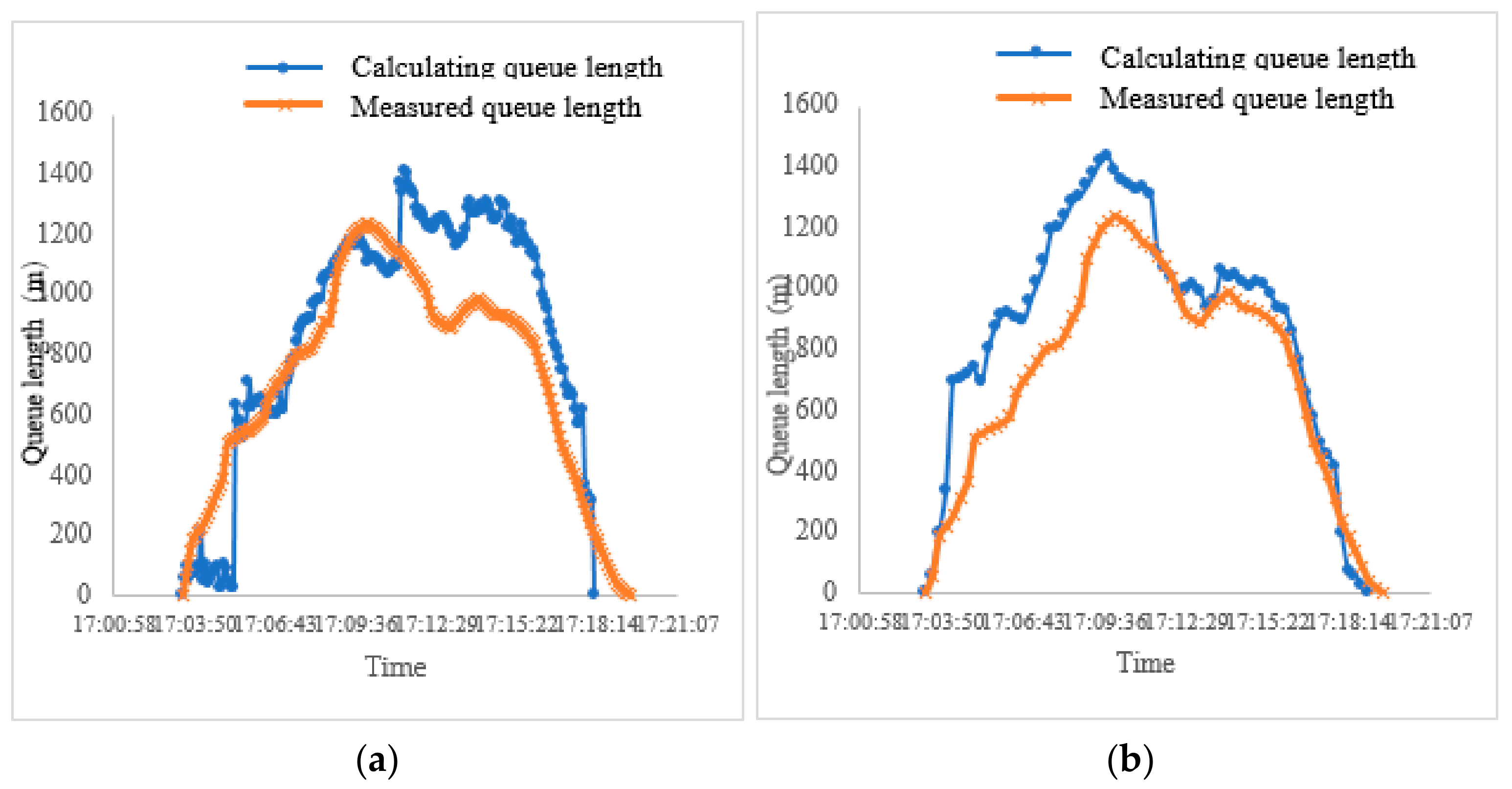
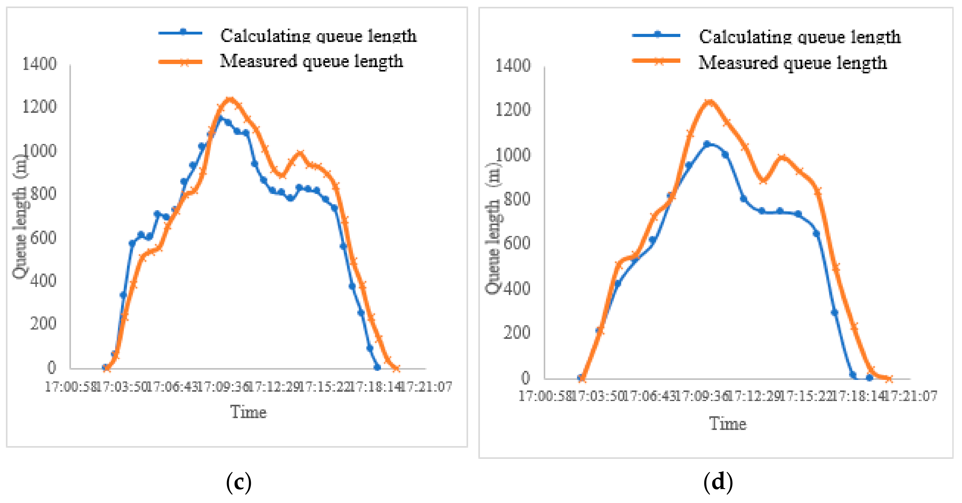
To validate the accuracy of the real-time queue-length calculation results at different time intervals, the calculated queue length is compared to the measured queue length when the time intervals are 5, 15, 30, and 60 s. Figure 15 depicts the results.

Table 4. Comparison of accuracy rate at different time intervals.

Time Intervals T/s	Maximum Queue-Length Accuracy	Whole-Process Queue-Length Accuracy
5	78.38%	64.01%
15	84.73%	69.27%
30	93.62%	83.05%
60	85.96%	73.11%

shows the accuracy of the maximum queue length and the overall process queue length.

The results show that when the time interval T is 5 s, the model’s estimated queue length differs significantly from the measured queue length. When T is 15 s, the estimated queue length is generally longer than the measured queue length; when T is 30 s, the estimated queue length is generally consistent with the measured queue length. When T is 60 s, the estimated queue length is usually less than the measured queue length. In general, the maximum queue length and overall process queue-length calculation accuracy are highest when the time interval T is 30 s; 60 s and 15 s are lower.

The data collected with a 5 s time interval is smoothed and filtered. Because the moving average’s window length is 30 s and 60 s, the difference is not significant, and the accuracy of the whole-process queue length with a value of 90 s is lower than the former two.

Table 5. Comparison of accuracy of different time intervals after smoothing with a window length of 30 s.

Time Intervals T/s	Maximum Queue-Length Accuracy	Whole-Process Queue-Length Accuracy
5	86.16%	76.41%
15	85.74%	75.09%
30	81.08%	72.56%
60	72.91%	59.46%

shows the maximum queue length and the accuracy of the whole-process queue length at different time intervals after smoothing the flow and density data with a window length of 30 s.

The results show that after smoothing the flow and density data with a window length of 30 s, the maximum queue-length accuracy increases from 78.38% to 86.16% when the time interval T is 5 s, and the overall process queue-length accuracy increases from 64.01% to 76.41%. When the time interval is 15 s, the maximum queue-length accuracy increased from 84.73% to 85.74%, and the overall process queue-length accuracy increased from 69.27% to 75.09%. When the time interval T is 5 s and 15 s, the accuracy of T taking 30 s and 60 s is reduced, indicating that the data moving average can improve the accuracy of the maximum queue length and the overall process queue length.

3.4. Model Accuracy Analysis

3.4.1. Time Interval Analysis

Because of the randomness of vehicle arrival, the flow and density data extracted at different time intervals differ significantly, as does the real-time queue length calculated from this. The value of the optimal time interval T is examined in order to improve the model’s accuracy. The flow, density, speed, and other data from an accident in the Qingdao Jiaozhou Bay Subsea Tunnel on 1 May 2019 were extracted. The accident happened around 10:09 a.m., and it ended around 10:20 a.m. The length of the queue is calculated by taking the time interval T of 5, 15, 30, and 60 s. Figure 16 depicts the estimation results, and

Table 6. Comparison of queuing length accuracy at different time intervals T.

Time Intervals T/s	Maximum Queue-Length Accuracy	Whole-Process Queue-Length Accuracy
5	71.47%	53.63%
15	72.64%	68.22%
30	95.62%	84.34%
60	86.27%	76.15%

depicts the accuracy of different time intervals T.

The results show that when the time interval T is 5 s, the model’s estimated queuing length differs significantly from the measured queuing length, and the accuracy of the maximum queuing length and the overall process queuing length is 71.47% and 53.63%, respectively. When T is set to 15 s, the estimated queue length is longer than the measured queue length, and the maximum queue-length accuracy and overall process queue-length accuracy are 72.64% and 68.22%, respectively. When the time interval T is 30 s, the estimated queue length agrees well with the measured queue length. The maximum queue length and total process queue-length accuracy are 95.62% and 84.34%, respectively. When T is 60 s, the estimated queue length is slightly greater than the measured queue length. The maximum queue length and total process queue-length accuracy are 86.27% and 76.15%, respectively. In general, the maximum queuing length and the total process queuing length have the highest accuracy when the time interval T is 30 s; the accuracy for 60 s and 15 s is lower. The error is relatively large when the time interval is 5 s. This is because, during the 5 s time interval, the flow and road density values in some collected sections are zero or fluctuate randomly, resulting in a large error in model estimation. To reduce random error, the statistical time interval of 5 s data are smoothed.

3.4.2. Data Sliding Smoothing Analysis

The flow and density data with a time interval of 5 s in statistics are processed by moving average based on the characteristics of large dispersion and volatility. After smoothing the data, the queue length for three groups of traffic and density data is estimated using the sliding average window lengths of 30, 60, and 90 s. To determine the best smoothing window length and whether the time interval T of the data in each group can be estimated, 5, 15, 30, and 60 s of data are taken. The measured queue length is compared to the queue length obtained after unsmoothing, smoothing for 30 s, smoothing for 60 s, and smoothing for 90 s, which are shown in

Table 7. Comparison of queue-length accuracy.

Time Intervals T/s	Unsmoothing		Smoothing for 30 s		Smoothing for 60 s		Smoothing for 90 s
	Maximum Queue-Length Accuracy	Whole-Process Queue-Length Accuracy	Maximum Queue-Length Accuracy	Whole-Process Queue-Length Accuracy	Maximum Queue-Length Accuracy	Whole-Process Queue-Length Accuracy	Maximum Queue-Length Accuracy	Whole-Process Queue-Length Accuracy
5	71.47%	53.63%	94.86%	81.89%	94.36%	81.76%	93.55%	77.87%
15	72.64%	68.22%	90.08%	82.23%	93.22%	80.27%	92.87%	76.74%
30	92.22%	84.34%	94.29%	82.02%	91.92%	72.05%	89.38%	74.64%
60	86.27%	76.15%	62.06%	68.98%	64.00%	67.91%	63.33%	63.66%

.

Table 7 shows that when the time interval T is 5 s, the accuracy rate is significantly increased after smoothing the data with a 5 s time interval. Smoothing the 30, 60, and 90 s produces similar results. The accuracy of the maximum queue length is 94.86%, 94.36%, and 93.55%, respectively, and the accuracy of the whole-process queue length is 81.89%, 81.76%, and 77.87%, respectively. The rule is consistent with that of 5 s when T is 15 s, which increases the precision of queue-length estimation. Results of 30, 60, and 90 s smoothing are comparable. Maximum queue-length accuracy is 90.08%, 93.22%, and 92.87%, respectively, while whole-process queue-length accuracy is 82.23%, 80.27%, and 76.74%. When the time interval T is between 30 and 60 s, the accuracy falls. It demonstrates that when the time interval T is between 5 and 15 s, smoothing the flow and density data can increase the model’s estimation accuracy. However, when the time interval is between 30 and 60 s, the model’s estimation accuracy cannot be increased because there is no significant difference between the sliding average window lengths of 30, 60, and 90 s. This might be the case because the time interval’s intrinsic value is greater than those of 5 and 15 s. The time-varying law of flow and density is hidden after moving average processing, which lowers the model’s accuracy.

3.5. Compared with the Input and Output Model

The input–output model is a common method for estimating the length of highway vehicle queue (uninterrupted traffic flow vehicle queue), as described in References [27,28,29,30,31]. The traditional input–output model determines the number of vehicles queuing in a certain section by estimating the difference between the number of vehicles arriving and leaving in a period of time, and then divides the vertical queuing length by the queuing vehicle density to obtain the queuing vehicle length in space. After the accident, the formula for estimating the difference between the number of vehicles arriving and leaving at moment $t$ and estimating the queue length of vehicles are as follows.

$$Q(t)={\displaystyle \underset{0}{\overset{t}{\int }}{Q}_{\mathrm{in}}dt}-{\displaystyle \underset{0}{\overset{t}{\int }}{Q}_{\mathrm{out}}}\mathrm{d}t$$

(24)

$$l(t)=\frac{Q(t)}{K_{\mathrm{queue}}(t)}$$

(25)

In the Formulas (24) and (25), $Q(t)$ expresses the difference in the number of vehicles arriving and departing at time $t$; $Q_{\mathrm{in}}$ represents the number of vehicles arriving upstream in the congestion area; $Q_{\mathrm{out}}$ represents the number of vehicles leaving the congestion area; $K_{\mathrm{queue}}(t)$ represents the queuing traffic density in the congested area; and $l(t)$ represents the vehicle queue length at time t.

In an actual traffic environment, it is difficult to obtain the continuous value of traffic variables, and the detector can only obtain the discrete value of traffic flow variables. In this paper, Formula (25) is discretized, and the discrete form shown in Formula (26) is obtained:

$$l(t)={\displaystyle {\sum }_{m=1}^n{T}_{\mathrm{m}}\frac{Q_{\mathrm{in}}^{}(t)-Q_{\mathrm{out}}(t)}{K_{\mathrm{queue}}^{}(t)}},n=\left[\frac{t-t_{\mathrm{A}}}{T}+1\right]$$

(26)

The comparison between the calculated queue length results for the shock-wave model, the input and output model developed in this paper, and the measured queue length is shown in Figure 17.

Table 8. Accuracy comparison between the proposed model and the input–output model.

Time Intervals T/s	Maximum Queue-Length Accuracy	Whole-Process Queue-Length Accuracy
model in this paper	93.62%	83.05%
input–output model	87.24%	73.85%

compares the shock-wave model’s accuracy to that of the input and output model.

4. Conclusions

This paper established a vehicle queuing length estimation method based on the traffic-flow shock wave by using measured data to examine the evolution law of vehicle congestion queuing throughout the entire process of traffic accidents in extra-long tunnels. Following are the particular conclusions:

(1)

Using the monitoring video data in the long tunnel, the maximum queue-length estimation model based on the traffic-flow shock-wave theory and the whole-process queue-length estimation model based on real-time data input were constructed based on an analysis of the evolution law of the queue length during the entire process of traffic accidents in the tunnel. The effect of data acquisition interval and data smoothing on the model’s precision was investigated. The relevant parameters in the model are defined in Appendix A.

(2)

According to the results, the model’s accuracy is greatest when the traffic flow data with an acquisition time interval T of 30 s are not smoothed; the accuracy for the maximum queue length and the total process queue length are 92.22% and 84.34%, respectively. The data smoothing procedure does not improve the model’s highest accuracy, but it has a significant effect when the time interval is between 5 and 15 s. There is no significant effect of sliding window length on the results.

(3)

Example verification demonstrates that the accuracy of the maximum queue-length estimation model based on shock-wave theory is 92.34%, and that the accuracy of the whole-process queue-length real-time estimation model based on shock-wave theory is 83.05%, reflecting the change rule of vehicle queue length under various control measures in real time. The accuracy of the whole-process queue-length estimation model presented in this paper is 83.05%, whereas the accuracy of the input–output model is 73.85%. The accuracy of the maximum queue-length estimation model based on shock-wave theory is 93.62%, while the accuracy of the input and output model is 87.24%; therefore, the model presented in this paper is more applicable.

This paper examines the evolution law of traffic-accident vehicle queue length in the tunnel’s basic section. The follow-up study must analyze the evolution law of vehicle queue length in other sections, such as diverging and merging areas, and should consider the characteristics of traffic accident queue length in extra-long tunnels with different vehicle types, lanes, or bus proportions in order to improve the model’s accuracy for practical applications.

References

1. Wang, S.; Huang, W.; Lo Hong, K. Combining Shockwave Analysis and Bayesian Network for Traffic Parameter Estimation at Signalized Intersections Considering Queue Spillback. Transp. Res. Res. Res. Part C Emerg. Technol. 2020, 120, 102807. [Google Scholar] [CrossRef]
2. Huang, W.; Hu, Y. A modified cell transmission model considering queuing characteristics for channelized zone at signalized intersections. Phys. A Stat. Mech. Its Appl. 2022, 605, 127977. [Google Scholar] [CrossRef]
3. Wang, D.B.; Yang, G.C.; Tian, Z.; Wei, D. Traffic Queue Length Estimation at Permissive Left-Turn Signalized Intersections with Probabilistic Priority. J. Transp. Eng. Part A Syst. 2022, 148, 04022107. [Google Scholar] [CrossRef]
4. Biswas, P.K.; Khan, S.M.; Piratla, K.; Chowdhury, M. Development and Evaluation of Statistical and Machine-Learning Models for Queue-Length Estimation for Lane Closures in Freeway Work Zones. J. Constr. Eng. Manag. 2023, 149, 04023023. [Google Scholar] [CrossRef]
5. Li, J.; Wang, P.; Li, B.L.; Wei, X.Z. Method for Estimation of Vehicle Queues Length Based on Probability Theory. J. Jiangsu Univ. Nat. Sci. Ed. 2020, 41, 557–561. [Google Scholar]
6. Latifi, H.; Goodarzi, M.J.; Amini, N.; Gilandeh, M.M.; Ali, S.S. Modelling of Queue Length in Freeway Work Zones–Case Study Karaj-Tehran Freeway. Promet-Traffic Transp. 2021, 33, 49–59. [Google Scholar]
7. Pan, Y.; Luo, J.; Chen, J.Z.; Zhang, Q. Study on Decision Technology of Traffic Congestion and Evacuation in a Highway Tunnel. Chin. J. Undergr. Space Eng. 2019, 114, 303–309. [Google Scholar]
8. Huang, Y.L. Research on Traffic Accident Impact and Evacuation Strategy of Expressway Tunnel. Master’s Thesis, Chang’an University, Xi’an, China, 2018. [Google Scholar]
9. Yang, G.C.; Tian, Z.; Wang, D.B.; Xu, H. Queue Length Estimation for a Metered On-ramp Using Mesoscopic Simulation. Transp. Lett. 2018, 11, 570–579. [Google Scholar] [CrossRef]
10. Amini, Z.; Pedarsani, R.; Skabardonis, A.; Varaiya, P. Queue-length Estimation Using Real-time Traffic data. In Proceedings of the 2016 IEEE 19th International Conference on Intelligent Transportation Systems, Rio de Janeiro, Brazil, 1–4 November 2016. [Google Scholar]
11. Wang, Y.; Zhang, D.B.; Zhang, Y. GPS Data Mining at Signalized Intersections for Congestion Charging. Comput. Econ. 2022, 59, 1713–1734. [Google Scholar]
12. Liu, D.B.; An, C.C.; Yasir, M.; Lu, J.; Xia, J.X. A Machine Learning Based Method for Real-Time Queue Length Estimation Using License Plate Recognition and GPS Trajectory Data. KSCE J. Civ. Eng. 2022, 26, 2408–2419. [Google Scholar] [CrossRef]
13. Li, A.J.; Tang, K.S.; Dong, K.R. Estimation of Queuing Length at Signalized Intersections using Low-frequency Point Detector. J. Transp. Inf. Saf. 2018, 36, 57–64, 95. [Google Scholar]
14. Chen, Q.; Li, M.; Wang, C.C. Cycle-Based Estimation on Lane-Level Queue Length at Isolated Signalized Intersection Using License Plate Recognition Data. J. Transp. Eng. Part A Syst. 2023, 149, 04022123. [Google Scholar] [CrossRef]
15. Tan, C.F.; Wu, H.; Tang, K.; Tan, C.P. An Extendable Gaussian Mixture Model for Lane-Based Queue Length Estimation Based on License Plate Recognition Data. J. Adv. Transp. 2022, 2022, 1–14. [Google Scholar] [CrossRef]
16. Tang, K.S.; Wu, H.; Yao, J.R.; Tan, C.P.; Ji, Y.B.B. Lane-based queue length estimation at signalized intersections using single-section license plate recognition data. Transp. B Transp. Dyn. 2022, 10, 293–311. [Google Scholar] [CrossRef]
17. Sheng, Z.; Xue, S.; Xu, Y.; Li, D. Real-Time Queue Length Estimation with Trajectory Reconstruction Using Surveillance Data. In Proceedings of the 16th International Conference on Control, Automation, Robotics and Vision, Shenzhen, China, 1 June 2020. [Google Scholar]
18. Aljamal, M.A.; Abdelghaffar, H.M.; Rakha, H.A. Real-Time Estimation of Vehicle Counts on Signalized Intersection Approaches Using Probe Vehicle Data. Inst. Electr. Electron. Eng. 2021, 22, 2719–2729. [Google Scholar] [CrossRef] [Green Version]
19. Umair, M.; Farooq, M.U.; Raza, R.H.; Chen, Q.; Abdulhai, B. Efficient Video-based Vehicle Queue Length Estimation using Computer Vision and Deep Learning for an Urban Traffic Scenario. Processes 2021, 9, 1786. [Google Scholar] [CrossRef]
20. Wei, L.; Li, J.H.; Xu, L.W.; Gao, L.; Yang, J. Queue Length Estimation for Signalized Intersections under Partially Connected Vehicle Environment. J. Adv. Transp. 2022, 2022, 1–11. [Google Scholar] [CrossRef]
21. Comert, G.; Begashaw, N. Cycle-to-cycle queue length estimation from connected vehicles with filtering on primary parameters. Int. J. Transp. Sci. Technol. 2022, 11, 283–297. [Google Scholar] [CrossRef]
22. Liu, H.; Liang, W.; Rai, L.; Teng, K.; Wang, S.L. A Real-Time Queue Length Estimation Method Based on Probe Vehicles in CV Environment. IEEE Access. 2019, 7, 20825–20839. [Google Scholar] [CrossRef]
23. Tan, C.P.; Yao, J.R.; Tang, K.S. Queue Length Distribution Estimation at Signalized Intersections Based on Sampled Vehicle Trajectory Data. China J. Highw. Transp. 2021, 34, 14. [Google Scholar]
24. Zhang, W.B.; Ye, J.Y.; Bai, Z.S.; Li, X.Y. Queue Length Estimation and Accuracy Assessment Method for Intersections Based on Trajectory Data. China J. Highw. Transp. 2022, 35, 10. [Google Scholar]
25. Gao, K.; Han, F.; Dong, P.; Xiong, N.X.; Du, R.H. Connected Vehicle as a Mobile Sensor for Real Time Queue Length at Signalized Intersections. Sensors 2019, 19, 2059. [Google Scholar] [CrossRef] [PubMed] [Green Version]
26. Jing, Q.; Li, K. Estimating Queue Length under Connected Vehicle Technology: Using Probe Vehicle, Loop Detector, Fused Data. Transp. Res. Rec. 2018, 2366, 35–39. [Google Scholar]
27. Sharma, A.; Bullock, D.M.; Bonneson, J.A. Input-output and Hybrid Techniques for Real-time Prediction of Delay and Maximum Queue Length at Signalized Intersections. Transp. Res. Rec. J. Transp. Res. Board 2007, 2035, 69–80. [Google Scholar] [CrossRef] [Green Version]
28. Yi, P.; Tian, Z.Z.; Zhao, Q. Consistency of Input-output Model and Shock Wave Analysis in Queuing and Delay Estimations. J. Transp. Syst. Eng. Inf. Technol. 2008, 8, 146–152. [Google Scholar]
29. Wang, Y.J.; Xu, J.M.; Li, W.Y. Estimation Model of Maximum Queue Length for Traffic Congestion at Urban Intersections. West. China Commun. Sci. Technol. 2009, 2, 84–90. [Google Scholar]
30. Liu, H.X.; Wu, X.K.; Ma, W.T.; Hu, H. Real-time Queue Length Estimation for Congested Signalized Intersections. Transp. Res. Part C Emerg. Technol. 2009, 17, 412–427. [Google Scholar] [CrossRef]
31. Carlson, R.C.; Papamichail, I.; Papageorgiou, M.; Messmer, A. Optimal Mainstream Traffic Flow Control of Large-scale Motorway Networks. Transp. Res. Part C Emerg. Technol. 2010, 18, 193–212. [Google Scholar] [CrossRef]
32. National Research Council (U.S.). Highway Capacity Manual; Transportation Research Board: Washington, DC, USA, 2010.
Figure 1. Spatial and temporal distribution of flow, density, and velocity in the whole accident process. (a) Spatial and temporal distribution of flow, (b) Spatial and temporal distribution of density, (c) Spatial and temporal distribution of velocity.
Mathematics 11 01773 g001
Figure 2. Flow–density following an accident in the extra-long tunnel.
Mathematics 11 01773 g002
Figure 3. Traffic flow following an accident in the extra-long tunnel.
Mathematics 11 01773 g003
Figure 4. Diagram of flow–density after a traffic accident in the extra-long tunnel.
Mathematics 11 01773 g004
Figure 5. Diagram of traffic flow after traffic control in the extra-long tunnel.
Mathematics 11 01773 g005
Figure 6. Diagram of flow–density after traffic control in the extra-long tunnel.
Mathematics 11 01773 g006
Figure 7. Diagram of traffic flow when vehicles meet queued vehicles after traffic control.
Mathematics 11 01773 g007
Figure 8. Diagram of flow–density after traffic accident clearance in the extra-long tunnel.
Mathematics 11 01773 g008
Figure 9. Diagram of flow density after traffic accident clearance in the extra-long tunnel.
Mathematics 11 01773 g009
Figure 10. Diagram of flow density after traffic flow cleared by accident meets the saturated traffic flow in the extra-long tunnel.
Mathematics 11 01773 g010
Figure 11. Diagram of traffic flow when the queue dissipates.
Mathematics 11 01773 g011
Figure 12. Diagram of vehicle time–space running track.
Mathematics 11 01773 g012
Figure 13. Flow chart for implementation of queue length estimation following an accident in the extra-long tunnel.
Mathematics 11 01773 g013
Figure 14. Accident data analysis diagram for one-way three lane on one lane.
Mathematics 11 01773 g014
Figure 15. Comparison of vehicle queue length at different time intervals and measured queue length. (a) The time interval T is 5 s, (b) The time interval T is 15 s, (c) The time interval T is 30 s, (d) The time interval T is 60 s.
Mathematics 11 01773 g015aMathematics 11 01773 g015b
Figure 16. Comparison of calculation results of queue length at different time intervals. (a) The time interval T is 5 s, (b) The time interval T is 15 s, (c) The time interval T is 30 s, (d) The time interval T is 60 s.
Mathematics 11 01773 g016
Figure 17. Comparison of calculation results of queue length of different models.
Mathematics 11 01773 g017