Article

Spectral Analysis for Comparing Bitcoin to Currencies and Assets

by
Maria Chiara Pocelli
1,†,
Manuel L. Esquível
2,*,† and
Nadezhda P. Krasii
3,†
1
Department of Mathematics, School of Industrial and Information Engineering, Politecnico di Milano, Piazza Leonardo da Vinci, 32, 20133 Milano, Italy
2
Department of Mathematics, Centre for Mathematics and Applications, NOVA School of Science and Technology, Quinta da Torre, 2829-516 Caparica, Portugal
3
Department of Higher Mathematics, Faculty of Informatics and Computer Engineering, Don State Technical University, 344003 Rostov-on-Don, Russia
*
Author to whom correspondence should be addressed.
These authors contributed equally to this work.
Mathematics 2023, 11(8), 1775; https://doi.org/10.3390/math11081775
Submission received: 15 February 2023 / Revised: 27 March 2023 / Accepted: 30 March 2023 / Published: 7 April 2023
(This article belongs to the Special Issue Probability Theory and Stochastic Modeling with Applications)

Abstract

:
We present an analysis on variability Bitcoin characteristics that help to quantitatively differentiate Bitcoin from the state-owned traditional currencies and the asset Gold. We provide a detailed study on returns of exchange rates—against the Swiss Franc—of several traditional currencies together with Bitcoin and Gold; for that purpose, we define a distance between currencies by means of the spectral densities of the ARMA models of the returns of the exchange rates, and we present the computed matrix of the distances between the chosen currencies. A statistical analysis of these matrix distances is further proposed, which shows that the distance between Bitcoin and any other currency or Gold is not comparable to any of the distances between currencies or between currencies and Gold and not involving Bitcoin. This result shows that Bitcoin is essentially different from the traditional currencies and from Gold, at least in what concerns the structure of its variance and auto-covariances.

1. Introduction

Money, in general, is a transmitter of value through time and space (see [1] I.1.19). Money is also a reference for the expression of the exchange value of every commodity (see [1] I.2.22). There are some characteristics of classical forms of money that we must now recall. The usual forms of money are under the control of central banks. These usual forms of money, currencies, have a close relationship with the economies to which the central banks are in charge; Swiss, United States of America, Russian Federation and European Monetary Union, are, respectively, examples of a country, a federation of states, a federation of republics and an economic zone composed of several countries. Thus, the exchange rates of one of these currencies versus the others, tend to vary, in a kind of first-order perturbation, according to the variation of regional economic variables.
The exchange rates also vary as a kind of second-order perturbation attributed to noticeable events—for instance, military instabilities. For these currencies, the monetary mass circulating must be both an equivalent of goods that circulate in the regional economy (to which the currency is connected) and a representation of the value of all the credits that achieve maturity at a given date. In all these credits, one should count even those credits that balance out each other (see [2] p. 135).
Considering a constant intrinsic value of the precious metals—such as silver or gold—and all other goods, we have that, for a usual form of money, the intrinsic value of bank notes decreases if the nominal value increases; this happens in light of the fact that the nominal value of bank notes does not represent the intrinsic value of some precious reference metal, and this may occur, for instance, by means of an increase in the quantity of these bank notes (see [2] pp. 142–143).
The hard connection between a usual form of money and the real economy has been recognized in many important classic economic works. For instance, in the third section of the third chapter of the first part of Capital, Karl Marx writes that: Just as the currency of money, generally considered, is but a reflex of the circulation of commodities, or of the antithetical metamorphoses they undergo, so, too, the velocity of that currency reflects the rapidity with which commodities change their forms…
In addition, concerning the relation between the quantity of money and the speed of the circulation of goods, the author we are quoting says The total quantity of money functioning during a given period as the circulating medium, is determined, on the one hand, by the sum of the prices of the circulating commodities and, on the other hand, by the rapidity with which the antithetical phases of the metamorphoses follow one another (see [3]). In more recent times, in the monetarist current of economy, Milton Friedman wrote that …the real quantity of money—the quantity of goods and services that the nominal quantity of money can purchase, or the number of weeks’ income to which the nominal quantity of money is equal (see [4] p. 1).
Bitcoin is a digital currency with many specific characteristics that distinguish it from usual currencies. In order to have a reasonable model for the exchange rate evolution of Bitcoin, some particular attributes should be considered. One of the most relevant characteristics of Bitcoin evolution is volatility (see Figure 1).
According to David Yermack, Bitcoin faces a number of obstacles in becoming a useful unit of account. One problem arises from its extreme volatility,… (see [5] p. 38). A first glimpse into the behaviour of the exchange rate and its variability—in this case, against the US Dollar—is captured in Figure 1 (graphic taken from the bitcoin.org site). Several features of this figure deserve a mention: the significant variability in the period from the middle of 2020 to February 2022 and, on the same period, the reduction in volume and in the rate of change (the lower graphic in blue).
These features certainly have an influence on the variance values that we will recover in the present work since one of our purposes is to study the variability of Bitcoin prices by comparing to the variability of state-owned currencies and a reference asset—Gold. According to Satoshi Nakamoto, the author that is credited for the creation of Bitcoin, …We have proposed a system for electronic transactions without relying on trust. … (see Nakamoto [6] p. 8). Given that it is common sense that the first and most important ingredient of any business is the building of mutual trust, the reality of present day existence of Bitcoin is another aspect that should deserve some analysis.
The market behaviour of Bitcoin has been studied under the perspective of its variability by several authors. In the following, we review some of the contributions that seem more relevant under the perspective of our approach both for the specific theme and for a broad context.
The book chapter [7] is an important review work that reports on the pairwise comparison of cryptocurrency characteristics with those of fiat currency and hard commodities, and it …synthesises methods and results from empirical research that investigate the nexus. One of the remarkable conclusions from the quoted work [8] is that …returns to cryptocurrencies are isolated from returns to currency and commodities, a result that we also find in our work with great significance. Another conclusion taken from a work using data in the period 2010–2017 (see [9]) is that Gold is found to be the second most important determinant for the full sample…; this also justifies the choice of Gold in our comparative study.
Comparative behaviours of crypto-currencies have also been studied recently. In [10], the authors compared the long term memory properties of seven cryptocurrencies—Bitcoin, Ethereum, Litecoin, Monero, Stellar, Tron and the EOS token—during and before the COVID-19 period, using high-frequency returns data, to find that the null hypothesis of true long memory is rejected for all series, implying that the persistence in the high-frequency cryptocurrency returns is not real and might be a spurious one, associated with some regime change during the sample period. Furthermore, the analysis is complemented with the estimation of the long-run correlation matrix of returns to find that, with the exception of Stellar, the remaining six crypto returns exhibit significant long-run correlations among each other, thus, justifying our consideration of only Bitcoin in this work.
The work [11] investigated …the contagious nature of tail events among cryptocurrencies and the mechanism by which tail risk permeates the cryptocurrency markets…, and this was achieved by constructing a network of tail risk spillovers among the most popular cryptocurrencies and identifying the most important shock-driving and shock-sensitive currencies in the network.
The work [12] analysed Bitcoin price volatility from the perspectives of Bitcoin’s own and external factors… by means of the structural vector autoregression (SVAR) model, the results showing that Bitcoin’s own factors play fundamental roles in Bitcoin price volatility, and the speculation factors have significant impacts on Bitcoin price volatility.
Comparative studies on the variances of the US Dollar, Bitcoin and Gold were performed in [13] using both an asymmetric GARCH model with explanatory variables and an exponential GARCH model. The author found that, in the perspective of explaining return, there is …volatility clustering and high volatility persistence similar to gold and concluded that …bitcoin and gold have similarities when it comes to the volatility of the return…. In the conclusions, it is said that both Bitcoin and Gold seem to react symmetrically to good and bad news but, …the frequency may be higher for bitcoin…
A detailed analysis of the importance of price jumps for Bitcoin is given in [14] showing—by GARCH modelling—that …the role of large movements is found to be stronger in the Bitcoin market than in the markets for crude oil and gold. A remarkable finding relates the evolution of variance to the occurrence of jumps also showing that the influence of jumps is larger in Bitcoin than in crude or Gold.
The work [15] provides an analysis of the main determinants of Bitcoin prices in a period of roughly 6 years ending in February 2019 using Auto Regressive Distributed Lag time-series model. The findings are on price variation, on one hand, that …macroeconomic and financial determinants… do not have a significant effect in short and long terms and, on the other hand, that …price variation is determined by demand variation.
Modelling the volatility of currencies and of Bitcoin has been the subject of recent works. In [16], the authors introduced, for a heterogeneous autoregressive model, a new model averaging coefficient estimator with the mean squared error of the coefficient to be minimised, and they provided inference by a double bootstrap since the relevant probability laws are unknown. This inference approach is similar to ours where, instead of bootstrap, we use a Monte Carlo simulation.
The source of any asset value variability is certainly multifactorial. In [17], the authors claim to not take a stand on the controversial question of what the fundamentals are behind Bitcoin, and they proceed to show that …the bitcoin market is largely like the stock market, with more investors who are more centrally placed on average earning higher returns than others…
We may conclude that there is a place for the study we now present towards a comparative study of the differences in variability between traditional state supported currencies, the crypto-currency Bitcoin and the asset Gold by means of power spectral distances. Let us briefly describe content and the main contributions of this work.
(i) 
In Section 2, we present the rationale for the choice of the reference currency against which all other currencies, Bitcoin and Gold are priced, and the choice of the state-backed currencies studied.
(ii) 
Next, in Section 3, we detail the ARMA process modelling of the returns of the exchange rates.
(iii) 
Section 4 introduces the distance between currencies and assets as the L 2 distance between Power Spectral Densities (PSD) (associated with currencies by means of ARMA modelling of the returns of the exchange rates against a fixed currency) and computes this distance between all pairs of currencies, Bitcoin and Gold. Next, we introduce a statistical test—based on the observed probability distribution of the returns of exchange rates—that allows, in the particular case chosen, to more precisely and firmly analyse the differences between currencies, Bitcoin and Gold.
(iv)  
In Section 5, we develop a result on the probability law of the distances of PSDs that justifies the empirical results presented in Section 4. These results encompass the case of asymptotically Gaussian-distributed PSD estimators. This result shows that, when considering observed spectral distances as random variables, the law of the distance of these spectral distances has, under assumptions that are verified in our study, a generalised Gamma distribution.
(v) 
Finally, in Appendix B, we study a variation of the assumption on the normality of returns of exchange rates of currencies that shows that this assumption may be acceptable in a preliminary study of differences between our chosen currencies.
The following are the main contributions of the study:
  • The introduction of the L 2 distance between Power Spectral Densities to differentiate the variance and auto-covariance behaviours of currencies, Bitcoin and the asset Gold.
  • The confirmation that an initial grouping of currencies, Bitcoin and Gold, by broad macro-economic criteria, reflects in the grouping driven by the L 2 distance between Power Spectral Densities (PSD).
  • The proposal of a statistical test to ascertain the difference of distances between the PSD associated with currencies, Bitcoin and Gold and of a mathematical result that justifies the modelling approaches followed.
  • Theorem 1 giving the probability law of the L 2 distance of observed spectral densities under assumptions that are general in the sense that these are assumptions verified with the data analysed in this work.

2. Foreign Exchange Markets and the Choice of Currencies and Assets to Study

Foreign Exchange is a form of currency exchange, consisting on the trading of one currency for another (see [18]). A price is associated with each currency pair. This price is the so-called exchange rate and it represents the value of a currency with respect to another.
In order to work with exchange rates, a reference currency has to be chosen as well as the currency objects of our analysis. In this section, the choice of these currencies is presented and explained.

2.1. On the Choice of the Reference Currency

Although there are hundreds of currencies, only a small number of them make up the vast majority of forex transactions. The most traded in the world are called the Majors, and they represent the largest share of the foreign exchange market (around 85%). These are:
  • United States dollar (Dollar), USD (United States).
  • Euro, EUR (Eurozone).
  • Pound Sterling, GBP (United Kingdom).
  • Australian dollar, AUD (Australia).
  • Canadian dollar, CAD (Canada).
  • Swiss franc, CHF (Switzerland).
  • Japanese yen, JPY (Japan).
It is reasonable to focus only on this group in order to select our reference currency. The most obvious choice would be the USD or EUR, since they are currently the most active currencies. However, the Global Crisis in 2008 and the COVID-19 crisis have led central banks around the world to roll out quantitative easing (QE) measures. These policies have had large and persistent effects on the Dollar/Euro exchange rate. As a result, investors began to flee to the Swiss franc, which is considered a safe-haven, since it offers protection from market shocks.
The dramatic surge of the CHF occurred in 2015, when the Swiss National Bank (SNB) removed the peg of 1.20 francs per euro, since it was no longer sustainable. The Swiss franc has emerged as one of the best alternatives to the US dollar and Euro. The strongpoint of the Swiss franc lies in the size of its related nation, Switzerland. Being a small country has enabled its economic system to become one of the world’s most advanced.
Moreover, Switzerland has no deficit, and this makes it self-reliant and stabilizes its currency. The Swiss franc is not backed by gold, meaning that the Swiss National Bank (SNB) can print any amount of currency without any need for a reserve. For all the above reasons, the reference currency chosen for our analysis was the Swiss franc.

2.2. On the Choice of Other Currencies and the Asset Gold

A further step was the selection of the other currencies to study with respect to the reference one. The USD is the home denomination of the world’s largest economy, the United States, and therefore it must be included among the currencies that we want to analyse. Similarly, all the remaining Majors must be considered.
On the other hand, the group of the greatest emerging economies of the world require special consideration. This group is composed of five countries, namely Brazil, Russia, India, China, South Africa, and it is known by the acronym BRICS. The notion behind the coinage of this acronym was that the BRICS cluster would grow to a size larger than the Majors by 2050, shifting the economic balance of power. That is, the largest global economic powers would no longer belong to the richest countries according to the income per capita. Therefore, the Brazilian real (BRL), the Russian Ruble (RUB), the Indian rupee (INR), the Chinese renminbi (CNY) and the South African rand (ZAR) are included in our analysis.
Likewise, the Israeli new shekel (ILS) has been gaining in strength against major currencies, such as the US dollar and the Euro, due, in large part, to high levels of foreign direct investment and to the strength of the tech sector. For this reason, this currency is also taken into consideration. In addition, the Swedish krona (SEK) and the Norwegian krone (NOK) is examined, as their corresponding countries benefit from a strong economy. Lastly, it is worthwhile to include the Polish zloty (PLN) to investigate possible ties with USD and EUR.
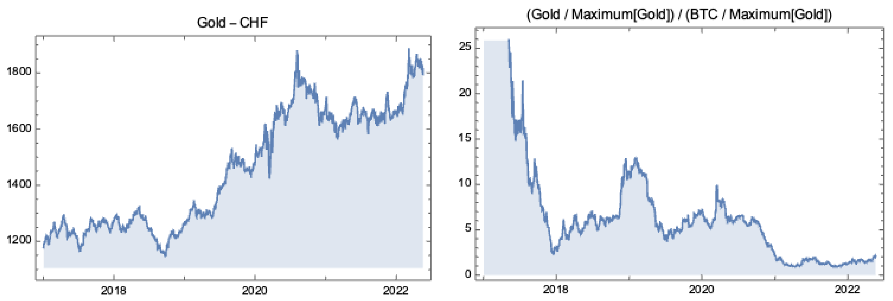
Finally, the asset gold (Gold) (XAU) is analysed, since it has been considered a highly valuable commodity for millennia acting as a reserve of value. As can be seen in Figure 2, the price evolution of Gold has similarities with the price evolution of Bitcoin—particularly for the most recent dates—leading to the natural question: how do Bitcoin and Gold compare using spectral densities?
Below, a summary of all the currencies considered for this study is shown receded by the indication of the distinctive class of the currency or asset that, by the arguments called in Section 2.1 and Section 2.2, justify their inclusion in this study.
  • The Majors: DOL, EUR, GBP, AUD, CAD and JPY.
  • The BRICS: BRL, RUB, INR, CNY and ZAR.
  • Independent Currencies: ILS, NOK, SEK and PLN.
  • Others: BTC and XAU.

3. Time-Series Analysis of the Data

Daily exchange rates against the Swiss franc (CHF) for all the currencies listed above were downloaded from Wolfram Financial Data Services. The study period goes from 1 January 2016 until 20 May 2022 when the effects of the Russian–Ukrainian conflict were not yet large enough to possibly disrupt stationarity. With those data, logarithmic returns were derived as follows:
r t = 100 log 10 e x _ r a t e t e x _ r a t e t 1 , t = 1 , . . . , # observations 1
Through (1), the time series of logarithmic returns was obtained for each currency. It is advisable to use returns for several reasons: first, to be able to compare different currencies and secondly to analyse dimensionless quantities. In the following Section 3.1, a preliminary analysis of those time series is proposed—keeping in mind the ARMA model application. For further information about the implemented techniques, see [19].

3.1. Stationarity Inspection

In order to correctly build the time-series model, it is necessary to first check the stationarity of our data. Here, this is achieved in two ways: statistically, using the augmented Dickey–Fuller test, and visually, looking at the autocorrelation plot of the data.
In the case of DOL/CHF time-series data, for example, the autocorrelation plot (Figure 3) shows that all lags are within the highlighted area in blue. Hence, we may assume stationarity, an assumption confirmed also by the Dickey–Fuller test result (rejection of the null hypothesis that the series is a unit root process). Similarly, stationarity was assessed for all the other currencies.

3.2. ARMA Modelling of the Returns of the Exchange Rates of Currencies against CHF

Since we assume our time-series data to be stationary, it is possible to model them as ARMA processes. We recall that, given a stationary process X, it is an ARMA(p,q) process if there exist a white noise W, a constant c and parameters a 1 , . . . , a p , b 1 , . . . , b q such that ([19] Ch8):
k = 0 p a k X n k = c + l = 0 q b l W n l , n Z , a 0 , b 0 = 1 .
Each time series was modelled as ARMA process with varying orders of p and q, from 1 to 4, and then the best fit was selected according to the Akaike information criterion (AIC). The results are shown in Table 1. It can be noticed that the variance of almost all the BRICS currencies and of Gold is one order of magnitude greater than the others (10–25% against 1–5%). On top of that, Bitcoin stands out from all the currencies reaching a variance of 279.7 % . A more complete analysis of this behaviour is further developed in Section 4 with the use of the spectral density.
The main conclusion that we can draw from this ARMA analysis is that, with the exception of Ruble, Bitcoin and Gold, the assets have variances of the same order of magnitude. Gold and Ruble both have variances one order of magnitude larger than the others assets, and Bitcoin has a variance two orders of magnitude larger than the other assets.

4. Comparing Currencies and Assets via the PSDs of Returns of Exchange Rates

In order to further investigate the variance of our time series, an application of spectral properties of ARMA processes is developed in this section (see [20,21] for the basic definitions).
If X is a wide sense stationary process with a summable covariance function, then there exists a function f X such that the auto-covariance function for the process is given by the formula:
R ( k ) = Cov ( X n , X n + k ) = [ π , π ] f X ( ω ) e i k ω d ω , n Z
and f X is called the power spectral density (PSD) of the process X (see [20] p. 185). Moreover, if k = 0 , it is possible to obtain the variance function of the process, which is:
R ( 0 ) = V ( X n ) = [ π , π ] f X ( ω ) d ω .

4.1. Power Spectral Density for the ARMA Process

In the case of an ARMA process and under the regularity hypothesis (see [20] p. 202), the PSD function is defined as:
f X ( ω ) = σ 2 2 π | Q ( e i ω ) | 2 | P ( e i ω ) | 2 ,
where Q ( z ) = k = 0 q b k z k and P ( z ) = k = 0 p a k z k , with a k and b k defined in (2). If z = e i ω = cos ( ω ) i sin ( ω ) , the squared moduli of Q ( z ) and P ( z ) become:
| Q ( z ) | 2 = k = 0 q b k 2 + 2 l = 1 q j = 0 l 1 b l b j c o s ( ( l j ) ω ) | P ( z ) | 2 = k = 0 p a k 2 + 2 l = 1 p j = 0 l 1 a l a j c o s ( ( l j ) ω ) .
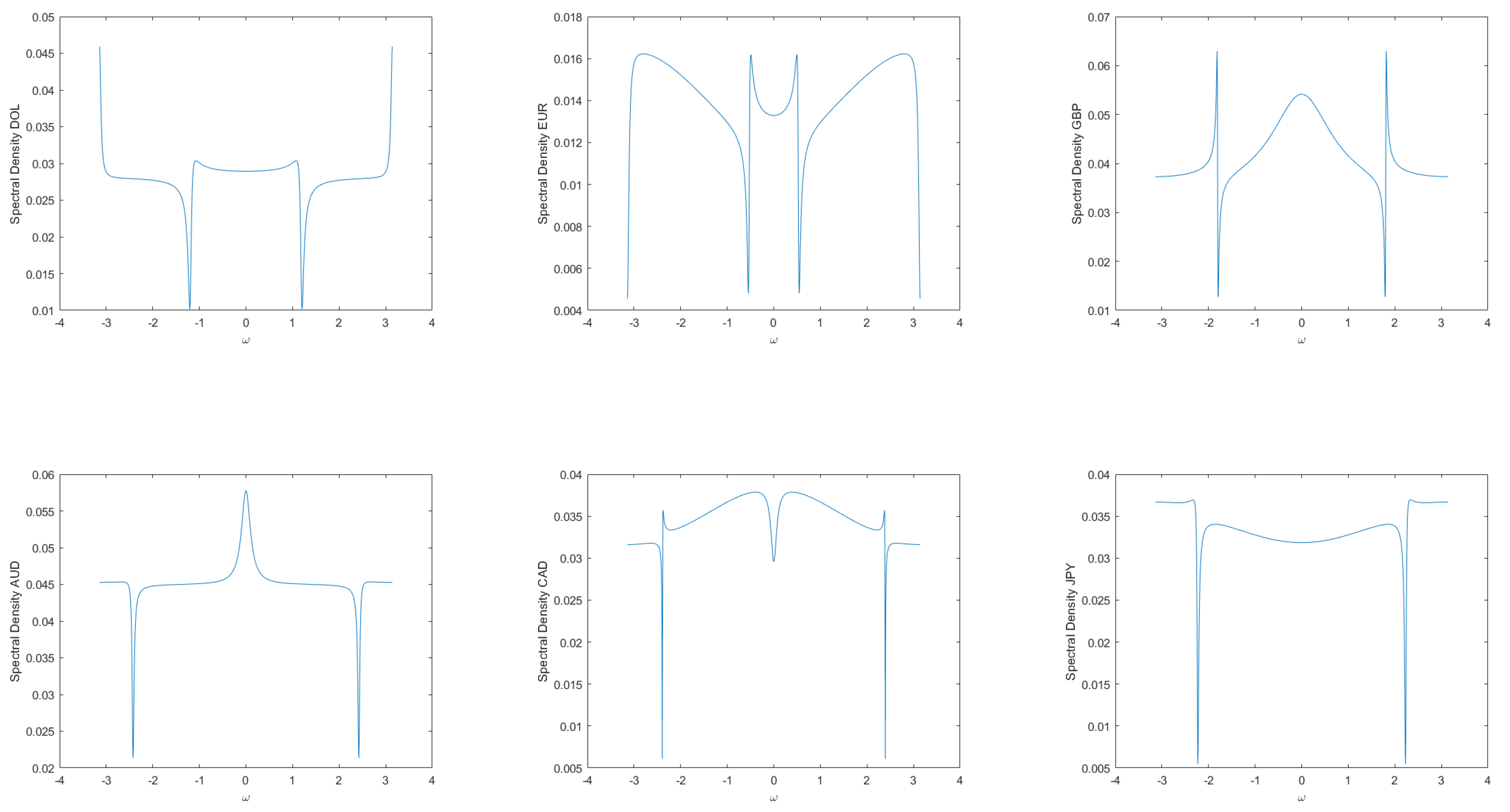
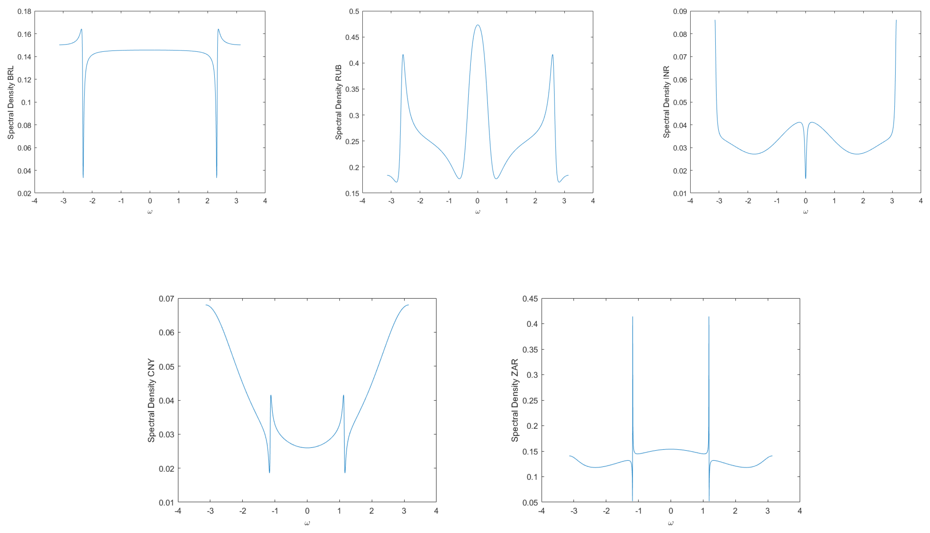
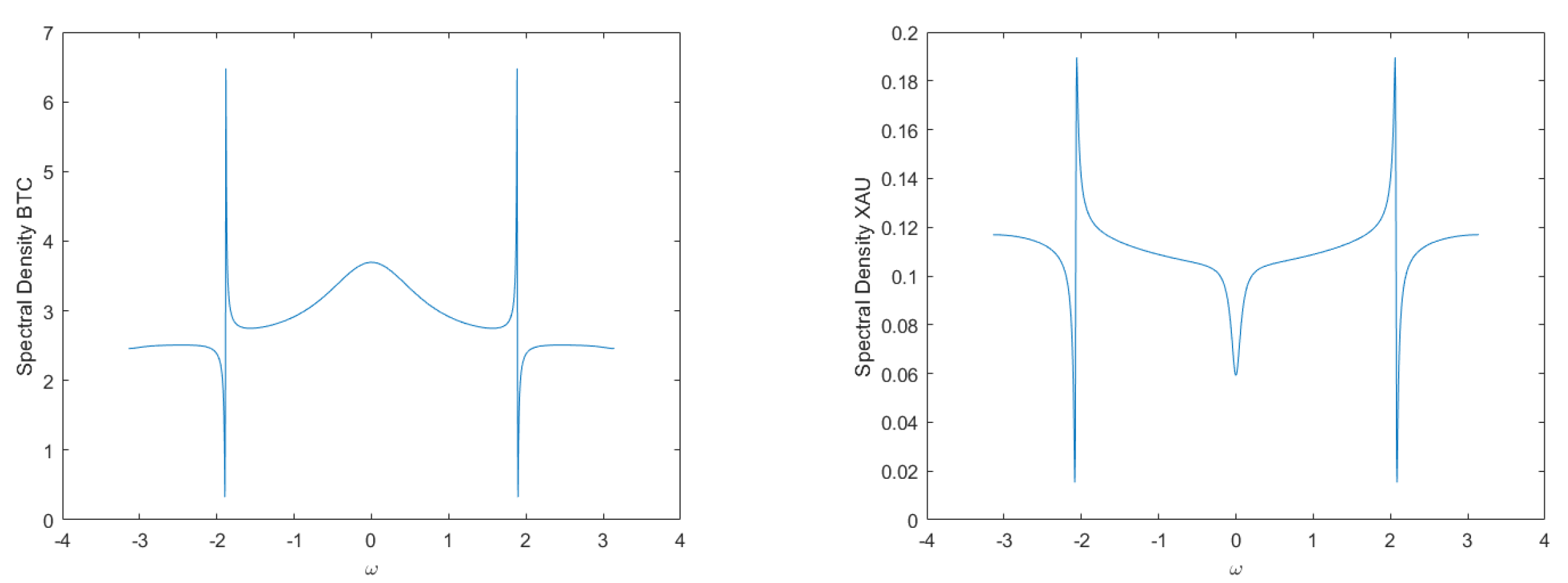
Through (5) and (6), it is possible to derive the PSD functions of our currencies, using the parameters obtained from the ARMA modelling. The plots of the computed functions, multiplied by 2 π , are shown in Appendix A.

4.2. Distance between Power Spectral Densities

For the purpose of comparing the obtained PSD functions, the L 2 ( [ π , π ] ) distance d is introduced. It is defined as ([20] p. 58):
d ( f , g ) = [ π , π ] | f ( ω ) g ( ω ) | 2 d ω 1 2 ,
with f , g L 2 ( [ π , π ] ) .
From (7), the distances between our PSD functions are computed, and the results are summarised in the symmetric matrix in Figure 4. The table in Figure 4 shows that the currencies can be divided into three groups:
  • A group of currencies for which distances among the elements of the group has order of magnitude equal to 2 (the Majors, the independent ones, INR and CNY).
  • Another group of currencies—disjoint from the first group—for which distances among the elements of the group has order of magnitude of 1 (the remaining BRICS and the asset Gold).
  • Bitcoin, which has a distance from the other currencies of around 7.
Figure 4. Matrix of distances.
Mathematics 11 01775 g004
This result confirms, in a more precise way, what was previously observed in Section 3.2.

4.3. A Statistical Test for Distances between PSDs Associated with Currencies and Assets

To show that the distances between PSD functions are meaningful, we introduce a statistical test procedure illustrated in a particular case. This is a Monte Carlo test procedure as it relies on Monte Carlo simulation of a test statistic in order to obtain its empirical distribution (see [22] or [23]). For the example studied, two currencies the US Dollar and the Euro, are taken. The test is performed in three different ways.
(a) 
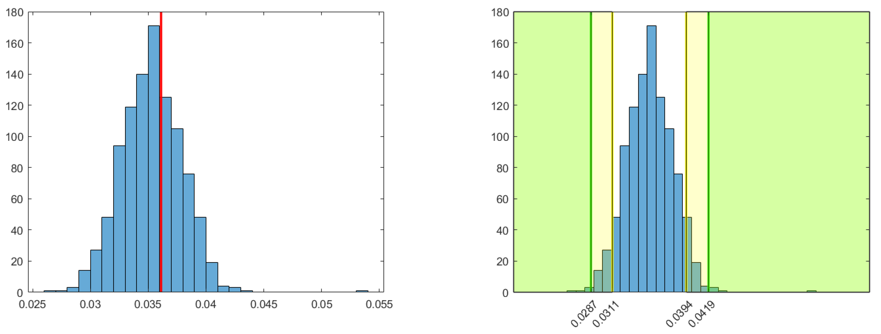
If normality of returns—derived from the exchange rates against the reference currency CHF—is assumed a priori (see Appendix B), the sample means μ ^ 1 , μ ^ 2 and the sample variances σ ^ 1 2 , σ ^ 2 2 of the returns of Dollar and Euro, respectively, are computed. With these values, a simulation of a sample of the returns of the two currencies is implemented, using Monte Carlo method. More precisely, an array of 2000 random numbers is generated from the normal distribution N ( μ ^ 1 , σ ^ 1 2 ) and from N ( μ ^ 2 , σ ^ 2 2 ) for Dollar and Euro, respectively. Then, ARMA modelling is executed and spectral density function is calculated for both the simulated returns. Finally, the distance between the computed PSDs is evaluated. This procedure—from the simulation—is repeated 1000 times, obtaining 1000 values of distances. The results are summarised in Figure 5. The red line represents the distance between Dollar and Euro computed using the real returns d * = 0.0361 (row 2, column 1 of the matrix in Figure 4).
With those data, it is possible to produce a statistical test with the null hypothesis:
H0: 
The spectral density of a given currency is either Dollars or Euros.
Significance levels α = 0.995 , 0.95 are used. The corresponding empirical quantiles are:
q 0.5 % = 0.0287 q 99.5 % = 0.0419
q 5 % = 0.0311 q 95 % = 0.0394 .
The steps for the test are the following:
(i)
Consider the distances of a currency d D o l , d E u r from Dollar and Euro, respectively, taken from the matrix in Figure 4.
(ii)
If ( d D o l q 1 α or d D o l q α ) and ( d E u r q 1 α or d E u r q α ), then the null hypothesis is rejected (see Figure 5).
(b) 
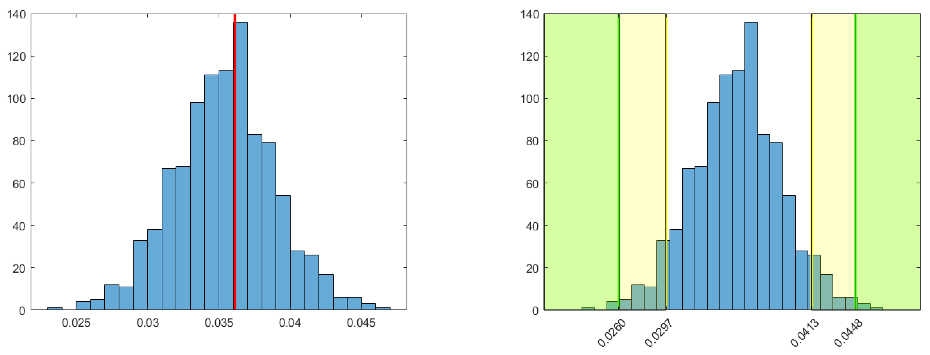
In order to avoid making assumptions about the distribution of the returns, the empirical cumulative distribution function is considered. This function is computed for both Dollar and Euro returns and 2000 random numbers are generated from it, for the two currencies. Then, the same steps as in Case (a) are repeated. The resulting histogram is shown below in Figure 6.
The new quantiles are given in Formulas (8) and (9), and the new rejection areas are shown in Figure 6.
q 0.5 % = 0.0260 q 99.5 % = 0.0448
q 5 % = 0.0297 q 95 % = 0.0413 .
(c) 
Another nonparametric representation of the probability density function of Dollar and Euro returns can be used, namely the kernel distribution. From this, a simulation is performed, and all the calculations are repeated. The new quantiles are given in Formulas (10) and (11), and the new rejection areas are shown in Figure 7.
q 0.5 % = 0.0285 q 99.5 % = 0.0462
q 5 % = 0.0313 q 95 % = 0.0427 .

4.4. A Discussion of the Results of the Statistical Tests

From Table 2, it is possible to conclude that it is better to use the ones of case (b) on the left-hand side and case (c) on the right-hand side as rejection areas. This is because the probability distribution of the distance is skewed. The normal approach in case (a) is a direct and quick method for the construction of the probability distribution of the distance.
The so-obtained left quantiles ( q 0.5 % and q 5 % ) were found to be similar to those of the kernel approach in case (c). Thus, the left tails of case (c) are close to the ones generated in case (a). The reason behind this lies, possibly, in the fact that a default kernel function—which is theoretically optimal for estimating densities for the normal distribution—was used in our computations.
Contrarily, the right quantiles ( q 99.5 % and q 99 % ) of the normal approach are substantially different from the values obtained using both (b) and (c) approaches. This means that empirical and kernel functions are able to more accurately capture the tail behaviour of the real data returns. The resulting quantiles of the distance distribution might be evidence of this: more extreme values for the real data returns entail more extreme simulated distances. However, the above observations are only possible interpretations of the results and contain questions for further research.
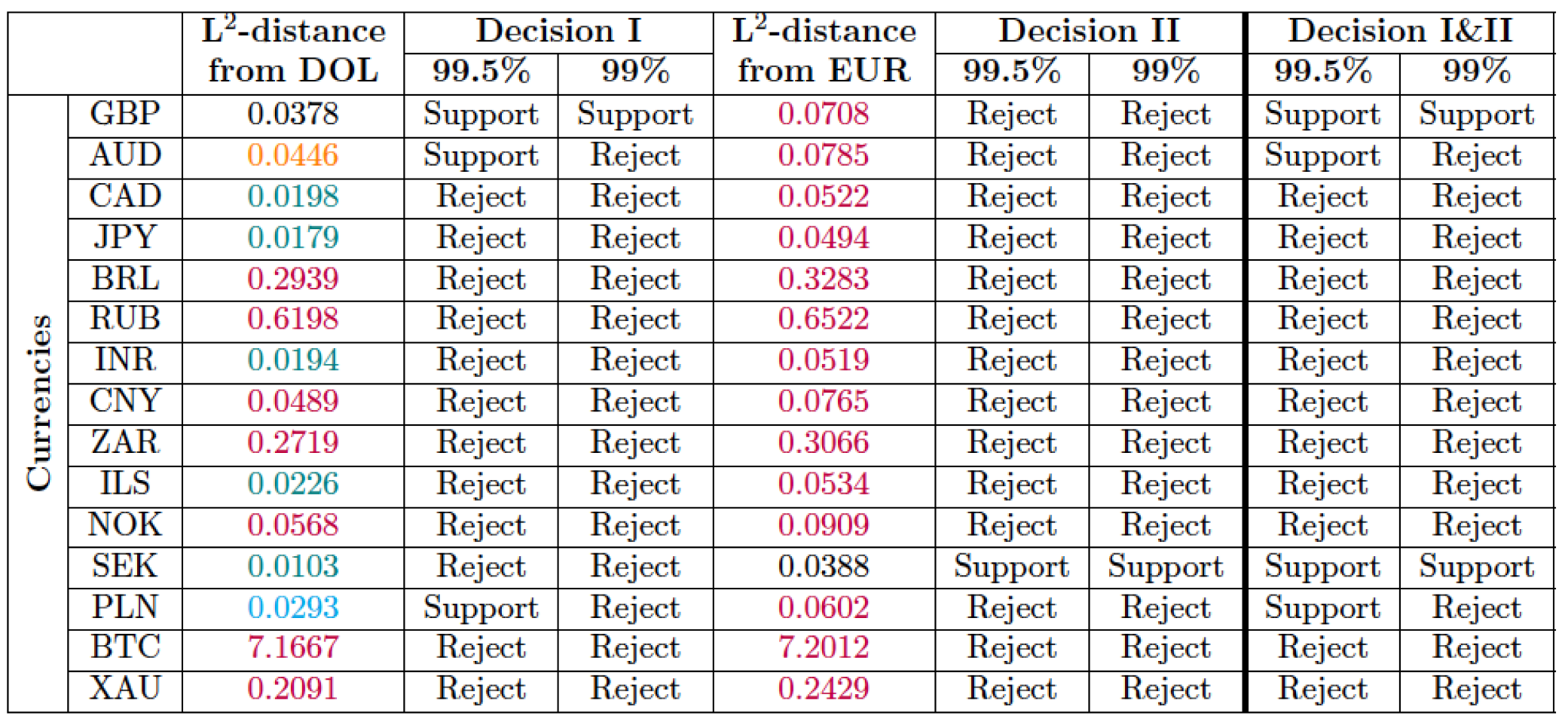
Taking into account the quantile values highlighted in Table 2, it is now possible to evaluate, for each currency, whether or not the null hypothesis can be rejected. The table in Figure 8 below displays the results of the test. The distances from Dollar and Euro of the majority of the currencies are in the rejection regions, even for very high levels of significance, meaning that there is a significant statistical separation between these currencies and both USD and EUR, based on the L 2 -distance. A remarkable observation is that the GBP seems to be close to USD and that SEK seems to be close to EUR; this fact should be the object of further investigation.

4.5. An Alternative to ARMA Modelling for Comparing Currencies and Assets: The Periodogram

Instead of computing a PSD function from the ARMA modelling, it is possible to consider an estimation of this function. In particular, in the following, we analyse the periodogram, which is a nonparametric estimate of the power spectral density of a stationary process under regularity assumptions. Its main advantage is that it does not need model fitting as was seen in Section 3. The periodogram is defined as ([20] Ch4.1.2):
P ( ω ) = 1 2 π N n = 0 N 1 x n e i ω n 2 , π ω π ,
where x n are the observations and N is the total number of observations. As in (6), it is possible to rewrite the squared modulus of the sum in the following way:
n = 0 N 1 x n e i ω n 2 = n = 0 N 1 x n 2 + 2 l = 1 N 1 j = 0 l 1 x l x j c o s ( ( l j ) ω )
Formulas (12) and (13) were used to compute the periodogram of all the currencies. Once all the periodogram functions are obtained, Formula (7) is applied, in order to find the new matrix of distances (Figure 9). Although the values in Figure 9 are slightly larger than those in Figure 4, it is still possible to divide the currencies in the same three groups previously presented.

5. On the Law of the Distance of Two Spectral Densities

In Section 4.3, we introduced a test for which it was necessary to have the probability distribution of the distance between two spectral densities. In order to consider such a distance as a random variable, we have several options. A first option is to consider the distance computed from the periodogram, such as in Section 4.5. In the case where the returns of the exchange rates may be assumed to be a stationary Gaussian process with zero mean and continuous spectra, the periodogram is known to have the chi-square distribution multiplied by some constant—essentially, a Gamma-distributed random variable (see [21] pp. 264, 270 or [24] p. 485).
In the present case, this option is not advisable since, as seen in Appendix B, the returns of the exchange rates do not satisfy normality assumptions. The results known for the law of the periodogram, not assuming normality of the returns of the exchange rates and in the form proposed in ([25] p. 194) does not seem of utility in our context.
A second option is to assume an ARMA model for the returns of the exchange rates and to inquire about the distribution of the coefficients of the ARMA model. Under regularity assumptions on the noise process, it is known that the coefficients of an ARMA process are asymptotically normal with zero mean and variances given by the spectral density (see [24] p. 482). It is also known that the Whittle-like estimators of the spectral density of a sufficiently regular ARMA process—since such a process is a wide sense stationary time series with an almost everywhere positive density (see [20] p. 226)—are consistent (see [26] p. 351) and asymptotically normal (see [24] p. 539, 540).
We observe that a connection between Gaussian and Whittle’s likelihoods is relevant for finite sample estimation; see [27]. From the results just quoted, it may be possible to deduce an asymptotic distribution for the distance of spectral densities. Nevertheless, since we observed good fittings of the actual data to Gamma distributions, we opted to formulate our results, ahead in Theorem 1, by stating directly the natural hypothesis needed instead of resorting to an asymptotic result.
In Section 4, we obtained samples of spectral densities for currencies Dollar US and Euro, let these be, respectively, f 1 ( · , ω ) and f 2 ( · , ω ) where, Ω being the probability space, the dot means that, for every ω Ω we have two functions given by t [ π , + π ] f 1 ( t , ω ) and also by t [ π , + π ] f 2 ( t , ω ) , which are spectral densities; we recall that these spectral densities are positive, continuous and even functions defined on [ π , + π ] .
We suppose that, for each t [ π , + π ] fixed, the random variables f 1 ( t , · ) and f 2 ( t , · ) are independent; this hypothesis is implicit in the Monte Carlo simulation procedure used in Section 4. We present, in the following, a result that justifies the computational results found. As a consequence of the construction method given above for the random processes f 1 , f 2 we have that the map defined by the L 2 distance, given by:
ω Ω d ( f 1 ( · , ω ) , f 2 ( · , ω ) ) 2 = π + π f 1 ( t , ω ) f 2 ( t , ω ) 2 d t = = 2 0 + π f 1 ( t , ω ) f 2 ( t , ω ) 2 d t ,
is a random variable. The next result provides a justification for the computational results found. In the following, we will use the parametrisation for X Γ ( α , β , γ , μ ) , a generalised Gamma-distributed random variable, with parametrisation given for its density f X by:
f X α , β , γ , μ ( x ) = γ e x μ β γ x μ β α γ 1 β Γ ( α ) x > μ 0 x μ ,
depending on parameters α , β , γ , μ (see [28] p. 388). As a consequence, we use a parametrisation for G Γ ( α , β ) , a Gamma-distributed random variable with parameters α , β , and the following expression for the density f G ,
f G α , β ( x ) = β α x α 1 e x β Γ ( α ) x > 0 0 x 0 .
We observe that f X α , β , 1 , 0 f G α , β .
Theorem 1
(On the probability law of L 2 distances of spectral densities). Consider the following assumptions which are justified by observed computational experiences.
1. 
Assumption A: a Gamma distribution provides a good fit for the random variable Q n given by:
Q k , n ( ω ) : = f 1 ( π k 2 n , ω ) f 2 ( π k 2 n , ω ) 2 Γ ( α k , n , β k , n ) ,
with the β k , n parameter of the Gamma distribution verifying 0 < β k , n 1 .
2. 
Assumption B: for arbitrarily values close to one another t t in [ π , + π ] , the random variables given by:
f 1 ( t , ω ) f 2 ( t , ω ) , f 1 ( t , ω ) f 2 ( t , ω )
are independent.
3. 
Assumption C: for n 1 , we have that, for some constants α , 0 < β 1 ,
π 2 n k = 0 2 n α k , n β k , n α β .
Then, d ( f 1 ( · , ω ) , f 2 ( · , ω ) ) Γ ( α , 2 β ) , 2 , 0 ) , that is, the the random variable d ( f 1 ( · , ω ) , f 2 ( · , ω ) ) admits a fitting by a generalised Gamma-distributed random variable.
Proof. 
Consider a standard discretisation numerical procedure that gives an approximation of the integral for large n:
0 + π f 1 ( t , ω ) f 2 ( t , ω ) 2 d t k = 0 2 n π 2 n f 1 ( π k 2 n , ω ) f 2 ( π k 2 n , ω ) 2 .
By Assumption A:, we are bound to find the distribution of the limit of a sum of Gamma-distributed random variables. We use the moment generating function and we determine the limit distribution of:
I n : = k = 0 2 n π 2 n f 1 ( π k 2 n , ω ) f 2 ( π k 2 n , ω ) 2 = k = 0 2 n π 2 n Q k , n .
We resort to the moment generating function of a Gamma-distributed random variable Γ ( α n , β n ) that is, in this case:
φ Q k , n ( t ) = E e t Q k , n = 1 ( 1 β k , n t ) α k , n .
As a consequence, under Assumption B, we have:
φ I n ( t ) = E e k = 0 2 n t π 2 n Q k , n = k = 0 2 n E e t π 2 n Q k , n = k = 0 2 n φ Q ( t π 2 n ) = k = 0 2 n 1 1 β k , n t π 2 n α k , n .
Under Assumption C, we obtain using 0 < β k , n 1 and 0 < β 1 ,
k = 0 2 n α k , n log 1 β k , n t p i 2 n k = 0 2 n α k , n β k , n t π 2 n α β t α log 1 β t ,
which, in turn, gives, in the limit:
lim n + φ I n ( t ) = lim n + k = 0 2 n 1 1 β k , n t π 2 n α k , n = 1 1 β t α .
This shows that d ( f 1 ( · , ω ) f 2 ( · , ω ) ) = 2 G ( ω ) with G ( ω ) Γ ( α , β ) , finally showing that d ( f 1 ( · , ω ) f 2 ( · , ω ) ) admits a fitting by a generalised Gamma-distributed random variable. In fact, we have that, given f G the density of G, the density of 2 G ( ω ) , let it be denoted by f 2 G ( ω ) , is given by f 2 G ( ω ) ( x ) = x f G ( x 2 / 2 ) . This equality, with a simple calculation using densities, shows that if G Γ ( α , β ) then 2 G ( ω ) Γ ( α , 2 β ) , 2 , 0 ) , that is, 2 G ( ω ) admits a fitting by a generalised Gamma distribution as announced. □
Remark 1
(On the interpretation of Assumption C). Formula (14) of Assumption C means that, for all orders n 1 of the resolution in the discretisation of the integral, the average of the Gamma distribution parameters for all the discretisation points should be constant. This assumption although with a straightforward interpretation is impossible to be fully verified; nevertheless, it can be verified for values n n 0 of the resolution order in the discretisation procedure of the integral, for n 0 1 sufficiently large.
Remark 2
(Testing equality of spectral distribution functions in the normal case). If we could assume the normality of the returns of the exchange rates it would be possible to test the equality of two spectral distribution functions with a simple computation (see [25] p. 198). As already noted this assumption is not valid in our case.

6. Conclusions

The returns of the exchange rates between various currencies and Swiss franc were calculated and modelled as ARMA processes. From this modelling, Power Spectral Densities were computed, and the L 2 -distance between them was introduced as a measure to compare the volatility behaviour of the returns. The resulting matrix of distances (see the table in Figure 4) clearly shows that there are three main different groups:
  • The Majors, the independent ones, INR and CNY.
  • The remaining BRICS and gold.
  • Bitcoin.
This grouping is similar to the grouping based in macro-economic criteria presented in Section 2, thus, showing that the variance and auto-covariance structure of returns of exchange rates of currencies is tied to the macro-economic properties of the owners of the currencies. Moreover, Bitcoin exhibits an extremely different quantitative behaviour when compared to one of the other currencies, revealing unique volatility properties.
An informed investor aware of the basic principles of Modern Portfolio Theory, such as those exposed in [29], has to take into consideration the extreme volatility properties of Bitcoin further revealed in this study. The study of the covariance structure for a portfolio, with similar methods to the one used in this work, can take advantage of modelling with vectorial ARMA processes (see [30]) and in cases where there is the possibility of regime switching VARMA models (see [31]).
An alternative approach presented is to directly estimate the Power Spectral Density with the periodogram, thus, avoiding ARMA modelling. These results add credibility to the ARMA modelling approach as the qualitative conclusions are identical, although the quantitative results in the matrix of distances (see the Table in Figure 9) are less precise. Figure 10 shows a comparison of the two approaches.
In both cases, three different groups are clearly detectable, as they exhibit three different shades of colour. Once again, it is noticeable that Bitcoin has standout values (yellow colour). It is also clear that the shades of colour in the graphic corresponding to the use of the PSD in the lefthand side are much more salient that those in the graphic corresponding to the use of the periodogram in the righthand side—also showing a loss of precision attached to the use of the periodogram already noticed in Section 4.5.
Furthermore, a statistical study was introduced. The empirical probability distribution of the L 2 -distance between the Power Spectral Densities of Dollar and Euro was constructed through performing a Monte Carlo simulation. The results were used to test and validate significant statistical separation between currencies basing on the L 2 -distance. Furthermore, a formal result was proven, which substantiates the probability distribution assumptions in this work.
As a stationary stochastic process can be characterised by its spectral density, the determination of the distance between the spectral distances introduced in this work is, in fact, a determination of a quantitative distance between (the ARMA models of) the returns of currencies. Furthermore, the statistical test introduced allows for a well-founded discussion of the separation in terms of the distance introduced between currencies and assets.
A natural question for further study is consider ways to obtain information on the joint variation of the returns of two currencies and or assets. A naive starting point may be the fact that, under some regularity assumptions, we can consider the product of ARMA processes (see [32]).

Author Contributions

Conceptualization, M.L.E.; methodology, M.L.E.; software, M.C.P. and M.L.E.; validation, M.C.P., M.L.E. and N.P.K.; formal analysis, M.L.E. and N.P.K.; investigation, M.C.P., M.L.E. and N.P.K.; resources, M.C.P., M.L.E. and N.P.K.; data curation, M.C.P.; writing—original draft preparation, M.C.P.; writing—review and editing, M.L.E., M.C.P. and N.P.K.; visualization, M.L.E., M.C.P. and N.P.K.; supervision, M.L.E.; project administration, M.L.E.; funding acquisition, M.L.E. All authors have read and agreed to the published version of the manuscript.

Funding

For the second and third authors, this work was partially supported through the project of the Centro de Matemática e Aplicações, UID/MAT/00297/2020, financed by the Fundação para a Ciência e a Tecnologia (Portuguese Foundation for Science and Technology). The APC was by supported by Fidelidade-Companhia de Seguras, S.A.

Data Availability Statement

Data for this study was collected with the Mathematica function “FinancialData” from Mathematica (see [33]). Mathematica™ is a Trade Mark from Wolfram Research, Inc., 100 Trade Center Drive, Champaign, IL 61820-7237, USA. Computations were performed initially with Mathematica and in a second round, for confirmations, with R software (see [34]).

Acknowledgments

This work was published with financial support from Fidelidade-Companhia de Seguras, S.A. to which the authors express their warmest acknowledgment. The authors express gratitude to the three referees for their comments, corrections and questions that led to a revised and better version of this work.

Conflicts of Interest

The authors declare no conflict of interest.

Appendix A. Power Spectral Densities

Figure A1. Power spectral density functions of the Majors.
Mathematics 11 01775 g0a1
Figure A2. Power spectral density functions of the BRICS.
Mathematics 11 01775 g0a2
Figure A3. Power spectral density functions of the independent currencies.
Mathematics 11 01775 g0a3
Figure A4. Power spectral density functions of Bitcoin and gold.
Mathematics 11 01775 g0a4
Remark A1.
It is clear that there is very significant information to be drawn from the spectral densities requiring a more sensible tool than the L 2 distance used in this work. One of the most remarkable features is the similar location of extrema, particularly in the case of Bitcoin and Gold, which should be placed in parallel with the graphic similarities observed in Figure 1 and Figure 2. We intend to pursue this analysis in future work.

Appendix B. Normality of Returns

The Dollar and Euro returns do not satisfy the normality assumptions that result from usual statistical tests. In this section, we present an attempt to transform data in a way so that a normality test is passed.
For both Dollar and Euro, returns r are grouped into sets of 12 elements. The mean of each set is saved in a vector R, and then the normality of R is tested and confirmed using the one-sample Kolmogorov–Smirnov test. Its sample mean μ ^ R and variance σ ^ R 2 are calculated, and the estimated mean and variance of the returns r correspond to μ ^ r = μ ^ R and σ ^ r 2 = 12 σ ^ R 2 supposing normality and independence of the elements of r.
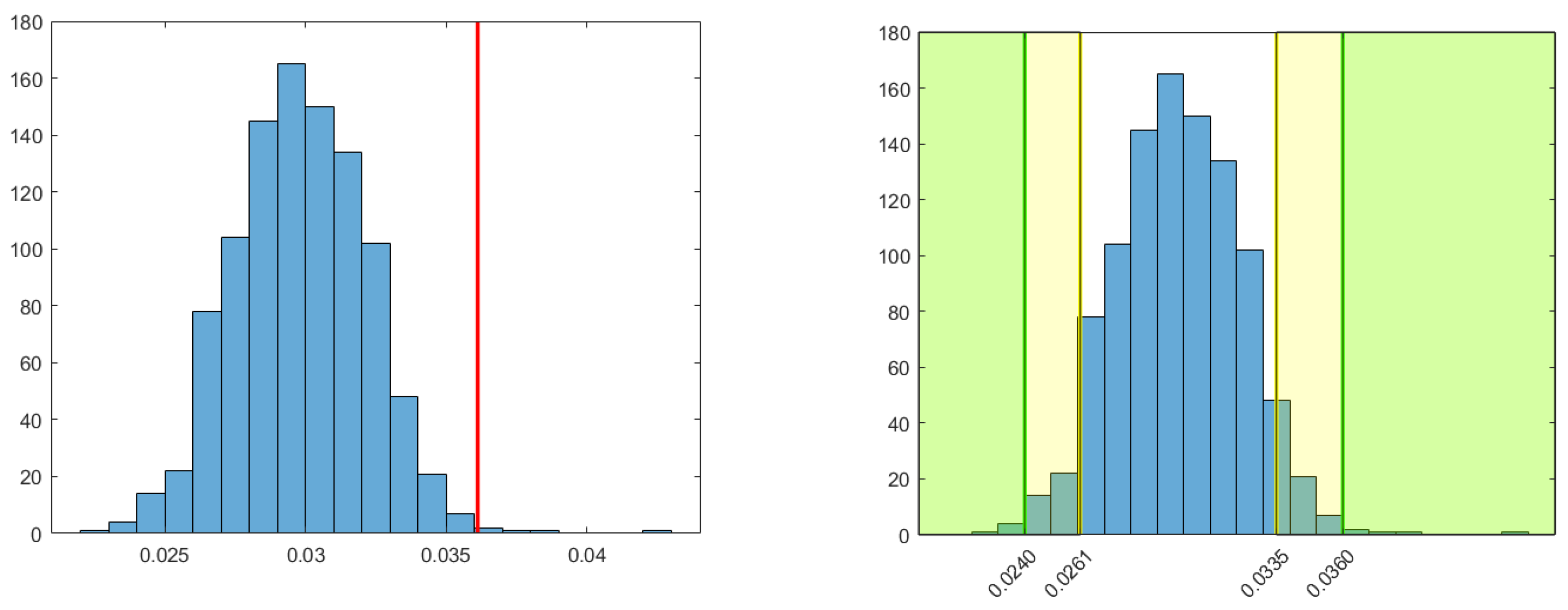
The new estimated means μ ^ 1 , μ ^ 2 and variances σ ^ 1 2 , σ ^ 2 2 of Dollar and Euro are obtained as specified above, and computations for the construction of the histogram are performed. The results are summarised in Figure A5. The average of the simulation data is not close to the value d * (red line), contrarily to the case in Figure 5.
Figure A5. New empirical probability distribution of the distance between Dollar and Euro (left) and new rejection areas for α = 0.995 (green) and α = 0.95 (yellow).
Mathematics 11 01775 g0a5
The quantiles for this approach are given in Formulas (A1) and (A2), and the new rejection areas are shown in Figure A5.
q 0.5 % = 0.0240 q 99.5 % = 0.0360
q 5 % = 0.0261 q 95 % = 0.0335
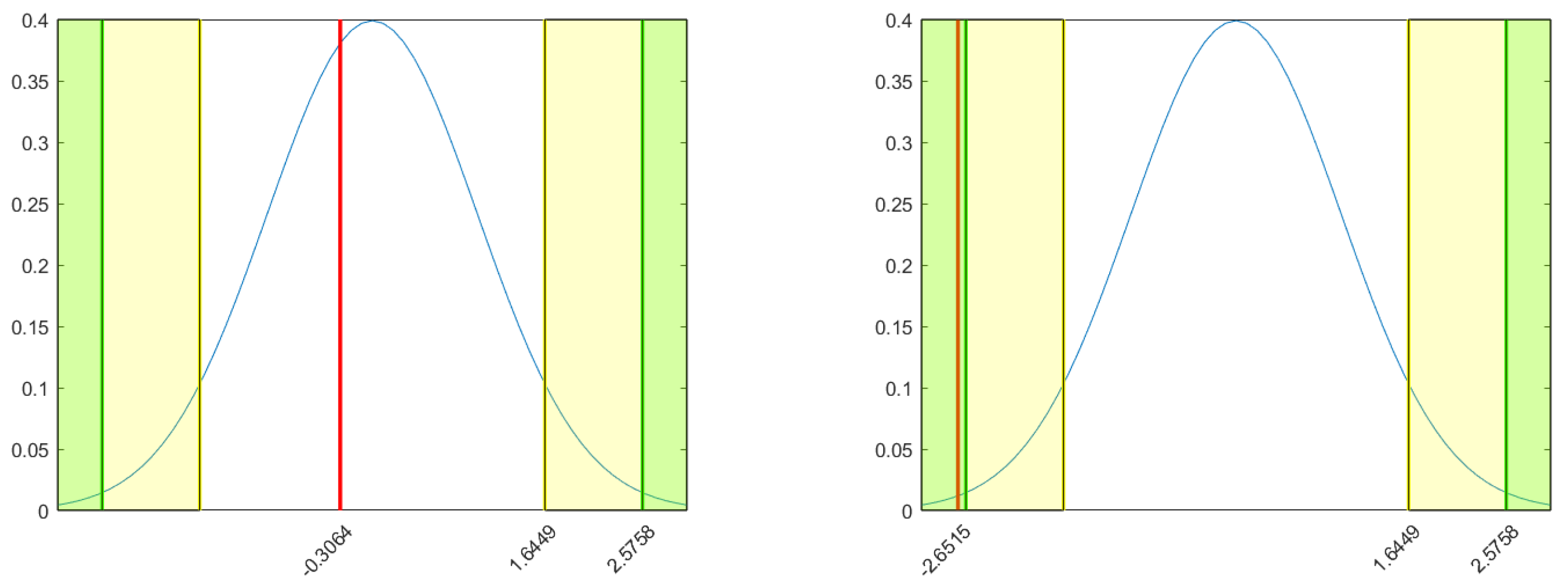
However, it can be demonstrated that there is no advantage in transforming the data. Indeed, it is possible to produce a statistical test to verify whether or not the mean values of the two histograms in Figure 5 and Figure A5 are the value d * .
The test is performed as follows. Once the mean μ and the variance σ 2 of the data visualised in the histogram, are obtained, the value z = ( μ d * ) / σ is computed and compared with the standard normal quantiles:
q 0.5 % = 2.5758 q 99.5 % = 2.5758
q 5 % = 1.6449 q 95 % = 1.6449 .
The null hypothesis can be written as:
H 0 : μ = z .
Figure A6 shows that H 0 is not rejected when normality is assumed a priori. This suggests that, despite Dollar and Euro returns not satisfying normality assumptions, it is possible to derive some results assuming normality.
Figure A6. Quantiles of the standard normal distribution and the value z (in red). On the (left), the case in which normality is assumed a priori. On the (right), the case in which data are transformed.
Mathematics 11 01775 g0a6

References

  1. von Mises, L. The Theory of Money and Credit; Liberty Fund: Indianapolis, Indiana, 1981. [Google Scholar]
  2. Mandel, E. Traité d’économie Marxiste; Number vol. 2 in Traité d’économie marxiste; Union Générale d’Éditions; René Julliard: Paris, France, 1962. [Google Scholar]
  3. Marx, K.; Mandel, E.; Fowkes, B. Capital: A Critique of Political Economy; Capital, Penguin Books Ltd.: Harmondsworth, UK, 2004. [Google Scholar]
  4. Friedman, M. The Optimum Quantity of Money, 1st ed.; Nobel Laureates in Economics; Aldine Transaction: Piscataway, NJ, USA, 1969; pp. xii, 296. [Google Scholar]
  5. Yermack, D. Chapter 2—Is Bitcoin a Real Currency? An Economic Appraisal. In Handbook of Digital Currency, 1st ed.; Chuen, D.L.K., Ed.; Academic Press: San Diego, CA, USA, 2015; pp. 31–43. [Google Scholar]
  6. Nakamoto, S. Bitcoin: A peer-to-peer electronic cash system. Bitcoin White Paper. Available online: https://bitcoin.org/bitcoin.pdf (accessed on 14 February 2023).
  7. Taheri, S.; Mann, J.; McWhirter, A. The Nexus between Cryptocurrencies, Currencies and Commodities: A Primer. In Cryptofinance; World Scientific Publishing Co. Pte. Ltd.: Singapore, 2022; Chapter 10; pp. 191–206. [Google Scholar] [CrossRef]
  8. Corbet, S.; Meegan, A.; Larkin, C.; Lucey, B.; Yarovaya, L. Exploring the dynamic relationships between cryptocurrencies and other financial assets. Econ. Lett. 2018, 165, 28–34. [Google Scholar] [CrossRef] [Green Version]
  9. Panagiotidis, T.; Stengos, T.; Vravosinos, O. On the determinants of bitcoin returns: A LASSO approach. Financ. Res. Lett. 2018, 27, 235–240. [Google Scholar] [CrossRef]
  10. Assaf, A.; Mokni, K.; Yousaf, I.; Bhandari, A. Long memory in the high frequency cryptocurrency markets using fractal connectivity analysis: The impact of COVID-19. Res. Int. Bus. Financ. 2023, 64, 101821. [Google Scholar] [CrossRef]
  11. Nguyen, L.H.; Chevapatrakul, T.; Yao, K. Investigating tail-risk dependence in the cryptocurrency markets: A LASSO quantile regression approach. J. Empir. Financ. 2020, 58, 333–355. [Google Scholar] [CrossRef]
  12. Xu, H.; Xu, X.; Wu, Z.; Guo, H.; Zhang, Y.; Wang, H. A Study on Bitcoin Price Volatility Based on the SVAR Model and Impulse Response Analysis. In Blockchain and Trustworthy Systems; Dai, H.N., Liu, X., Luo, D.X., Xiao, J., Chen, X., Eds.; Springer: Singapore, 2021; pp. 214–225. [Google Scholar]
  13. Dyhrberg, A.H. Bitcoin, gold and the dollar—A GARCH volatility analysis. Financ. Res. Lett. 2016, 16, 85–92. [Google Scholar] [CrossRef] [Green Version]
  14. Gronwald, M. Is Bitcoin a Commodity? On price jumps, demand shocks, and certainty of supply. J. Int. Money Financ. 2019, 97, 86–92. [Google Scholar] [CrossRef]
  15. Guizani, S.; Nafti, I.K. The Determinants of Bitcoin Price Volatility: An Investigation With ARDL Model. Procedia Comput. Sci. 2019, 164, 233–238. [Google Scholar] [CrossRef]
  16. Qiu, Y.; Wang, Z.; Xie, T.; Zhang, X. Forecasting Bitcoin realized volatility by exploiting measurement error under model uncertainty. J. Empir. Financ. 2021, 62, 179–201. [Google Scholar] [CrossRef]
  17. Tsang, K.P.; Yang, Z. Do connections pay off in the bitcoin market? J. Empir. Financ. 2022, 67, 1–18. [Google Scholar] [CrossRef]
  18. Lipton, A. Mathematical Methods for Foreign Exchange; A Financial Engineer’s Approach; World Scientific Publishing Co., Inc.: River Edge, NJ, USA, 2001; pp. xxii, 676. [Google Scholar] [CrossRef]
  19. Azencott, R.; Dacunha-Castelle, D. Series of Irregular Observations; Springer: New York, NY, USA, 1986. [Google Scholar]
  20. Brémaud, P. Fourier Analysis and Stochastic Processes; Springer: Cham, Switzerland, 2014; pp. xiii, 385. [Google Scholar]
  21. Koopmans, L.H. The spectral analysis of time series. In Probability and Mathematical Statistics, 2nd ed.; Academic Press, Inc.: San Diego, CA, USA, 1995; Volume 22, pp. xvi, 366. [Google Scholar]
  22. Dufour, J.M.; Khalaf, L. Monte Carlo Test Methods in Econometrics. In A Companion to Theoretical Econometrics; John Wiley & Sons, Ltd.: Hoboken, NJ, USA, 2003; Chapter 23; pp. 494–519. [Google Scholar] [CrossRef]
  23. MacKinnon, J.G. Bootstrap Hypothesis Testing. In Handbook of Computational Econometrics; John Wiley & Sons, Ltd.: Hoboken, NJ, USA, 2009; Chapter 6; pp. 183–213. [Google Scholar] [CrossRef] [Green Version]
  24. Anderson, T.W. The Statistical Analysis of Time Series; John Wiley & Sons: Hoboken, NJ, USA, 1971. [Google Scholar]
  25. Grenander, U.; Rosenblatt, M. Statistical Analysis of Stationary Time Series; John Wiley & Sons: New York, NY, USA; Almqvist & Wiksell: Stockholm, Sweden, 1957; p. 300. [Google Scholar]
  26. Brockwell, P.J.; Davis, R.A. Time Series: Theory and Methods; Springer Series in Statistics; Springer: New York, NY, USA, 2006; pp. xvi, 577, Reprint of the second (1991) edition. [Google Scholar]
  27. Subba Rao, S.; Yang, J. Reconciling the Gaussian and Whittle likelihood with an application to estimation in the frequency domain. Ann. Statist. 2021, 49, 2774–2802. [Google Scholar] [CrossRef]
  28. Johnson, N.L.; Kotz, S.; Balakrishnan, N. Continuous Univariate Distributions, 2nd ed.; Wiley Series in Probability and Mathematical Statistics: Applied Probability and Statistics; John Wiley & Sons, Inc.: New York, NY, USA, 1994; Volume 1, pp. xxii, 756. [Google Scholar]
  29. Benninga, S. Financial Modeling, 4th ed.; The MIT Press: Cambridge, MA, USA, 2014; pp. xxxi, 1111. [Google Scholar]
  30. Reinsel, G.C. Elements of Multivariate Time Series Analysis, 2nd ed.; Springer Series in Statistics; Springer: New York, NY, USA, 1997; pp. xviii, 357. [Google Scholar] [CrossRef]
  31. Cavicchioli, M. Spectral density of Markov-switching VARMA models. Econom. Lett. 2013, 121, 218–220. [Google Scholar] [CrossRef]
  32. Engel, E.M.R.A. A unified approach to the study of sums, products, time-aggregation and other functions of ARMA processes. J. Time Ser. Anal. 1984, 5, 159–171. [Google Scholar] [CrossRef]
  33. Wolfram Research, Inc. Mathematica, Version 12.3.1.0; Wolfram Research, Inc.: Champaign, IL, USA, 2022. [Google Scholar]
  34. R Core Team. R: A Language and Environment for Statistical Computing; R Foundation for Statistical Computing: Vienna, Austria, 2021. [Google Scholar]
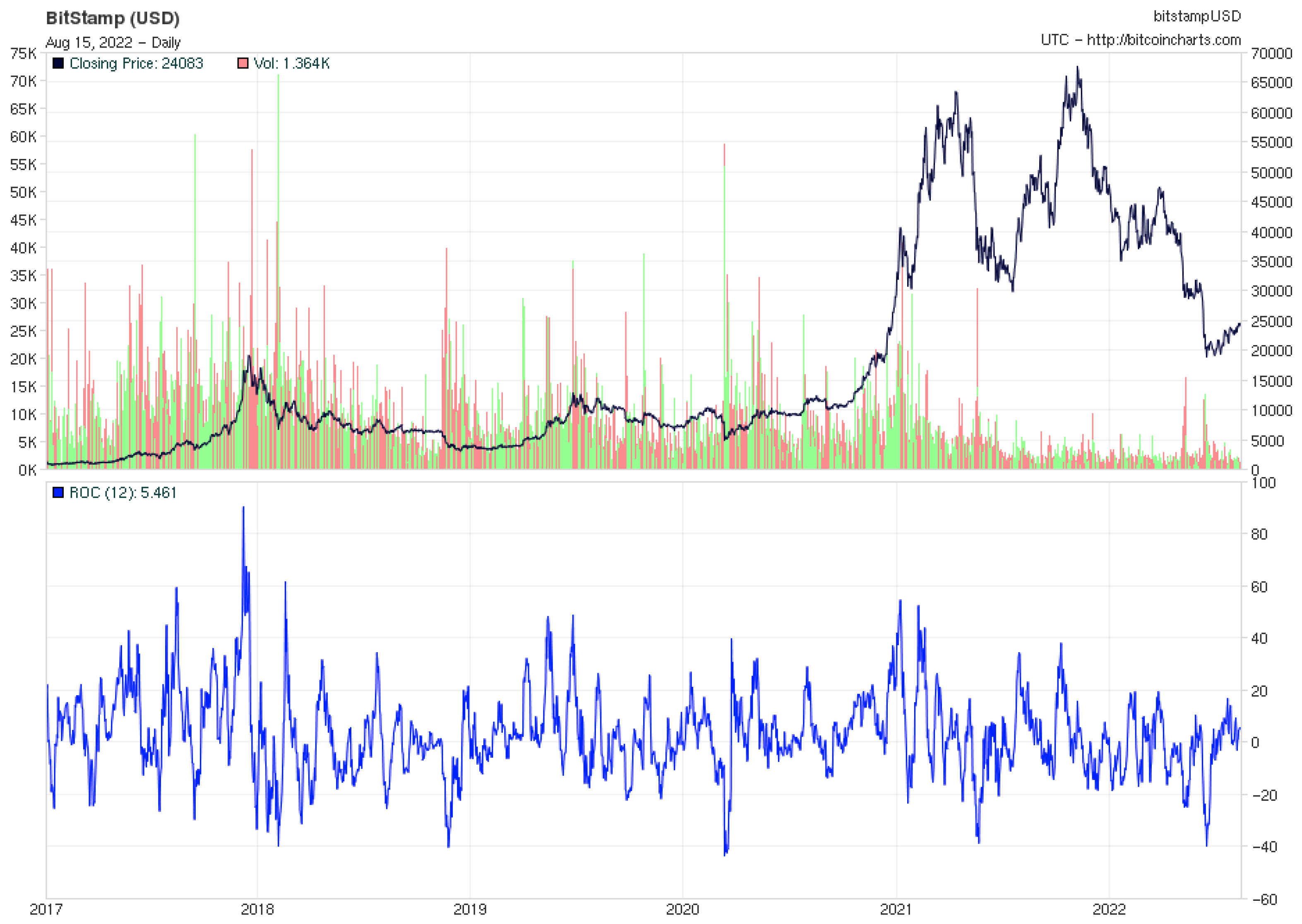
Figure 1. Price in US Dollars and the rate of change evolution from 2017 to the present.
Mathematics 11 01775 g001
Figure 2. Price of Gold from 2017 to the present (left) and ratio of normalised prices of Gold and Bitcoin (right).
Mathematics 11 01775 g002
Figure 3. Autocorrelation plot of the DOL/CHF time-series data.
Mathematics 11 01775 g003
Figure 5. Case (a): probability distribution of the distance between Dollar and Euro (left) and rejection areas for α = 0.995 (green) and α = 0.95 (yellow) (right).
Mathematics 11 01775 g005
Figure 6. Case (b): probability distribution of the distance between Dollar and Euro (left) and rejection areas for α = 0.995 (green) and α = 0.95 (yellow) (right).
Mathematics 11 01775 g006
Figure 7. Case (c): probability distribution of the distance between Dollar and Euro (left) and rejection areas for α = 0.995 (green) and α = 0.95 (yellow) (right).
Mathematics 11 01775 g007
Figure 8. Results of the statistical tests.
Mathematics 11 01775 g008
Figure 9. New matrix of distances.
Mathematics 11 01775 g009
Figure 10. Matrices of distances with scaled colours. On the left is the matrix obtained from PSD, and on the right is the matrix obtained from the periodogram.
Mathematics 11 01775 g010
Table 1. Best-fit ARMA processes for each currency.
DOLEURGBPAUDCADJPY
p333342
q343333
σ 2 0.02770.01400.04090.04500.03430.0333
BRLRUBINRCNYZAR
p24233
q24424
σ 2 0.14350.25140.03270.03910.1339
ILSNOKSEKPLN
p3414
q4414
σ 2 0.03400.04900.02900.0370
BTCXAU
p44
q43
σ 2 2.79700.1085
Table 2. Quantiles of cases (a), (b) and (c). The values for which it is harder to reject are coloured (the smaller values are on the left of the histogram, and the larger are on the right).
q 0.5 % q 5 % q 95 % q 99.5 %
(a) Normal0.02870.03110.03940.0419
(b) Empirical0.02600.02970.04130.0448
(c) Kernel0.02850.03130.04270.0462
Disclaimer/Publisher’s Note: The statements, opinions and data contained in all publications are solely those of the individual author(s) and contributor(s) and not of MDPI and/or the editor(s). MDPI and/or the editor(s) disclaim responsibility for any injury to people or property resulting from any ideas, methods, instructions or products referred to in the content.