Abstract
A new approach to the verification of current-state opacity for discrete event systems is proposed in this paper, which is modeled with unbounded Petri nets. The concept of opacity verification is first extended from bounded Petri nets to unbounded Petri nets. In this model, all transitions and partial places are assumed to be unobservable, i.e., only the number of tokens in the observable places can be measured. In this work, a novel basis coverability graph is constructed by using partial markings and quasi-observable transitions. By this graph, this research finds that an unbounded net system is current-state opaque if, for an arbitrary partial marking, there always exists at least one regular marking in the result of current-state estimation with respect to the partial marking not belonging to the given secret. Finally, a sufficient and necessary condition is proposed for the verification of current-state opacity. A manufacturing system example is presented to illustrate that the concept of current-state opacity can be verified for unbounded net systems.
MSC:
93-08
1. Introduction
In recent decades, with the rapid development of information technology and computer science, the security of cyber–physical systems has become a hot research direction in interdisciplinary areas, which include many human-built infrastructures. Discrete event systems (DESs) serve as the technical generalization of such human-made systems that are usually computer-integrated and evolve with the predefined regulations. Typically, almost all the production systems fall into this category. In discrete event systems, similar to controllability, observability, diagnosability, and detectability, opacity is one of the basic attributes of DESs [1], which reflects the confidentiality of a system. To be specific, when unauthorized external observers (or intruders) observe the evolution of the system, they cannot infer that the predicate representing secret information is true.
In the context of DESs, a secret predicate can be either a subset of the state space or a subset of the language generated by a system [2,3]. Opacity can be accordingly divided into two categories: state-based opacity and language-based opacity. Furthermore, state-based opacity can be categorized into current-state opacity (CSO) [4,5], initial-state opacity [6,7], k-step, and infinite-step opacity [8,9,10,11]. Opacity verification can be conducted in a centralized or decentralized framework [12], under different formalisms such as fuzzy or stochastic DESs [13,14].
In this work, the concept of current-state opacity is verified by using an unbounded system, i.e., the number of times a transition is triggered is no longer set with an upper limit. A basis coverability graph (BCG) is constructed to address the CSO verification of a DES modelled with unbounded Petri nets (UPNs); such a system cannot be modelled with a finite state automaton. A condition in [6] is extended, i.e., some unobservable transitions can be detected in a partially observed DES. Moreover, an external observer (or intruder) is assumed to know the overall structure and initial state of the unbounded net model, but only part of places can be observable, i.e., the number of tokens in such a place can be explicitly measured or counted. Under such a setting, it becomes much more challenging to estimate the current state of an unbounded system. This paper constructs a BCG for an unbounded Petri net to determine the possible current state of the system according to the derived quasi-observable transitions and partial observable places.
Compared with finite-state automata (FSA), Petri nets are a more popular tool for modelling and controlling DESs [15]. By changing the number of tokens in places, the system behaviors are observed for further investigations [16] of interesting system properties or behavior. Petri nets have been extensively used to study the diagnosability analysis [17,18], state estimation [19], and supervisory control of DESs. In [17], a programming problem is formulated to perform fault diagnosis in a bounded Petri net, while the work in [18] reports a verifier net to derive a fault diagnosis method for DESs.
However, the existing results in the framework of bounded Petri nets usually need to construct reachability graphs [17,18,19], which suffer from the notorious state explosion problem. In other words, it is difficult to enumerate all the states for real-world systems due to their large sizes [20]. To mitigate this issue, a new type of reachability graph is proposed by Cabasino et al. [21], called a basis reachability graph (BRG). The authors, as well as the followers in the DES domain, apply BRG to many DES problems such as fault diagnosis, diagnosability analysis, supervisory control, and critical observability, opacity verification and enforcement.
In the research on DESs based on Petri nets, there are few studies on unbounded net systems. Ushio et al. [22] reported a method of fault diagnosis by using a partially observed UPN, where all transitions are unobservable and partial places are observable. In [22], two diagnosers, a simple diagnoser and an -diagnoser, were constructed to analyze the diagnosability of an underlying system by monitoring the token counts and their changes in observable places. Moreover, the work in [23] improved the results in [18] by extending the diagnosability analysis in bounded net systems to unbounded net systems using a verifier net. In addition, when analyzing the state space of an unbounded net system, its coverability graph [24,25,26] has to be considered. In [27], Lefaucheux et al. extended the concept of BRGs to unbounded net systems. The authors analyzed the relationship between coverability sets and reachability sets. After the definition of BCGs was proposed, the relationship between BCGs and BRGs was further analyzed. Based on the proposed BCGs, the diagnosability analysis for unbounded net systems was significantly improved by the team who originally developed the notion of BRG with a deluge of results. For example, it was shown that an unbounded net system is diagnosable iff there does not exist any cycle in the BCG with the relevant set of fault transitions. However, the investigation of further applications of the BCGs is still open.
Opacity verification and enforcement have been extensively studied and applied to real applications [5,6,7,28,29], i.e., no matter what information is observed by a malicious intruder from outside, some non-secret information and secret information cannot be identified. In this case, the intruder cannot decide whether the possible current system states reasoned from the current observation so far belong to the pre-defined secret of the system.
In [30], the concept of opacity in finite transition systems was proposed for the first time, which was then extended to Petri nets [31]. For the verification of CSO, Tong et al. [4] used a BRG to verify the CSO of a bounded labeled Petri net, which was extended in [6] by representing a secret as generalized mutual exclusion constraints. In addition, a secret with no weakly exposed markings and uncertainty of the initial marking were also considered. The work in [5] verified the CSO in a partially observed bounded Petri net, where the unobservable transitions were divided into quasi-observable transitions and truly unobservable transitions, which were used to analyze the behavior of the system such that more information regarding the system evolution can be precisely captured. However, as far as we know, no work has been reported on the opacity verification of DESs modeled by UPNs.
In this paper, we touch upon the verification of opacity of a DES modeled with unbounded Petri nets by borrowing the methods in [5,6]. The major contributions of this work are stated as follows.
- A new type of basis coverability graph is proposed. The work by Lefaucheux et al. in [27] is extended to propose a new BCG based on the partially observable places only. In short, based on the number change of tokens in all observable places, the system can determine whether the (unobservable) transitions in their pre/post-sets are fired. This approach releases the frequently adopted assumption that observable transitions necessarily exist in a plant. Furthermore, this newly constructed BCG is readily applicable to the formulation of control laws for large and complex systems. A method of state estimation based on this BCG is also presented;
- A verification approach for CSO based on BCG is proposed. A sufficient and necessary condition is developed for the verification of opacity based on the current-state estimation and proves that the CSO can be verified in unbounded net systems.
This paper is organized into five sections. Section 2 conceptualizes partial markings and basis coverability graphs. In Section 3, we introduce a method to estimate the current state by using the newly proposed BCG. Section 4 details the verification of CSO in partially observed UPNs. To show that our method is effective and feasible, an example of a real-world system is shown in Section 5. Finally, the paper is concluded in Section 6.
2. Construction of BCG
The concepts of partial markings and BCGs are reviewed in this section, and a new type of BCG is proposed. Due to the limited space, we suppose that readers are familiar with the preliminaries of the Petri net theory and the related concepts. To facilitate the reading and understanding of this research, the Petri net notations and notions used in this paper can be seen in [32]. In addition, the system considered in this work is assumed to be self-loop free.
2.1. Partial Markings
A marking restricted to is represented by a vector with j entries, called the partially observable marking of the marking M [33]. Then, a partially observable marking (partial marking for simplicity) can be readily calculated by
where A is a matrix, called the observability mapping matrix with for , and the other entries are 0. Similarly, the matrix A is used to project a marking M of a Petri net onto a partial marking based on the set of observable places .
Example 1.
A marking of a partially observed UPN is denoted as . By assuming that the mapping matrix is
the partial marking of is , whose entries correspond to places , , and , respectively, i.e., , , and .
In order to construct the BCG for a UPN with partially observable markings, a coverability set of partial markings is defined as
Although all the transitions are assumed to be unobservable in a UPN in this paper, the transitions whose firing can be detected and inferred by the token changes in observable places are called quasi-observable transitions. Given an unbounded net system , the set of quasi-observable transitions is defined as
Similarly, the transitions that are not in are called truly unobservable transitions. Given an unbounded net system , the set of truly unobservable transitions is .
Given a transition sequence , we use to denote the natural projection with respect to quasi-observable transitions, i.e., , which is defined as
The inverse projection is defined as , i.e., consists of all transition sequences in whose observations are w.
Example 2.
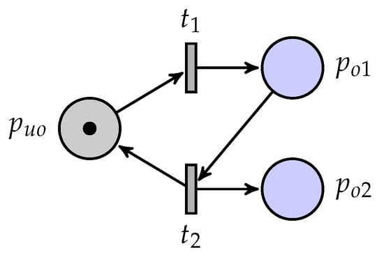
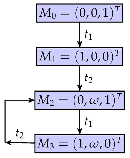
A partially observed unbounded Petri net is considered as shown in Figure 1, where is an unobservable place. Its coverability graph is shown in Figure 2, where a marking is denoted by . Note that is unbounded and that the set of quasi-observable transitions is .
Figure 1.
A partially observed unbounded Petri net.
Figure 2.
The coverability graph.
Note that, in this investigation, the number of tokens in unbounded places is denoted by . Therefore, if there are some unbounded places that are observable, the system’s administrators or intruders can detect the change in the number of tokens in these places. In simpler terms, for some unbounded places, which are denoted by , if they are observable, their pre-sets and post-sets are detectable and quasi-observable.
Algorithm 1 is used to identify the quasi-observable and the truly unobservable transitions in an unbounded Petri net. Moreover, given a quasi-observable string w and a partial marking , let us define the set of states that are possibly reachable by detecting and observing w and as
which is a collection of markings consistent with w and .
| Algorithm 1: Classification of transitions. |
 |
2.2. Basis Coverability Graph in Partially Observed UPNs
Different from the work in [27], where an approach based on the labeled Petri nets and their markings is proposed, the concepts of quasi-observable transitions, truly unobservable transitions, and partial markings are used to construct our novel BCGs. In addition, the definition of an unobservable transition subnet [6,20] is extended to truly unobservable transitions.
Definition 1.
Let be a UPN. Additionally, is a set of truly unobservable transitions. The truly unobservable subnet of N is obtained by removing , where and are the restrictions of and to , respectively. The incidence matrix of this subnet is denoted by .
Therefore, based on the above definition, we assume that the truly unobservable subnet is acyclic.
As shown in Figure 3, a partially observed UPN is considered. Table 1 and Figure 4 show the list of markings and its coverability graph, respectively, where a regular marking is denoted as .
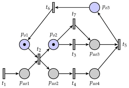
Figure 3.
An unbounded Petri net.

Table 1.
Markings list of Figure 3.
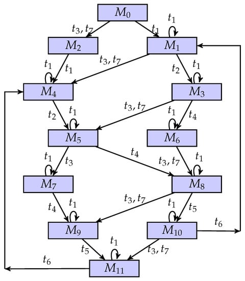
Figure 4.
A coverability graph of the unbounded net system.
Definition 2.
Given a partially observed UPN with its truly unobservable subnet being acyclic, a partial markings , and a transition ,
is defined as a set of explanations of quasi-observable transition at partial marking , and is defined as the corresponding set of explanation vectors.
Definition 3.
Given a partially observed UPN with the acyclic truly unobservable subnet, a partial marking , and a transition ,
is defined as a set of minimum explanations of quasi-observable transition at partial marking and is defined as the corresponding set of minimum explanation vectors.
Therefore, there necessarily exists a set of basis markings in a BRG regardless of whether the transition set of a labeled Petri net is partitioned [6]. However, in a partially observed UPN, the markings are no longer applicable to constructing the BCG. Instead, the partial markings are only used for this graph. In the following, the definition of a set of basis partial markings is proposed.
Definition 4.
For an unbounded net system and an initial partial marking , a set of basis partial markings is defined as follows:
- ;
- and , it holds , where .
In other words, the set of basis partial markings includes the initial partial marking and a set of all of the partial markings reachable by firing quasi-observable transitions and minimum explanations of truly unobservable transitions.
Based on the above definitions, an algorithm is proposed to construct a BCG for partially observed UPNs. We follow the work in [6] by using an NFA to represent the novel BCG, where is the set of basis partial markings, is a set of quasi-observable transitions, and is a transition function defined as .
Algorithm 2 can be briefly explained. In the first step, the set of basis partial markings is initialized at . For all non-visited basis partial markings and all quasi-observable transitions , we need to determine whether its minimum explanation vector is a nonempty set. If it is not empty, a new basis partial marking can be calculated. The algorithm runs repeatedly until all basis partial markings are calculated.
| Algorithm 2: Construction of BCG for a partially observed UPN. |
 |
Example 3.
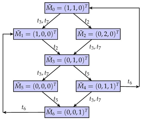
The partially observed unbounded Petri net is considered again as shown in Figure 3. Table 1 is the marking list of the net system, where a marking is denoted as ; Figure 4 is the coverability graph of the net system. The places , , , and are assumed to be unobservable. Therefore, the set of quasi-observable transitions is , and the others are truly unobservable transitions. Moreover, a new mapping matrix is assumed as
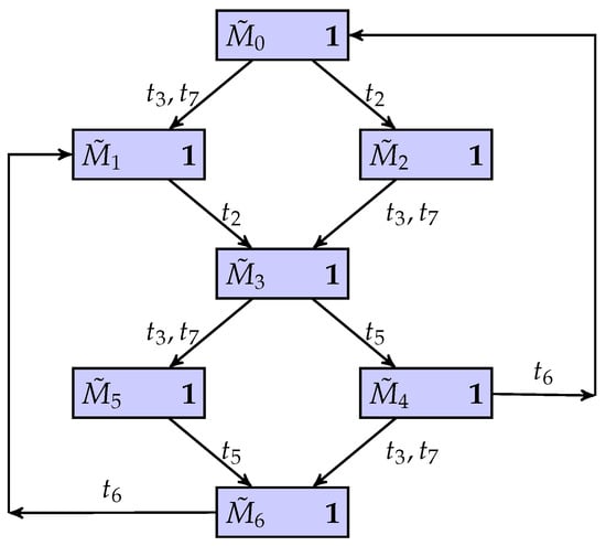
The novel BCG is shown in Figure 5. Since and are truly unobservable transitions, if an intruder observes a new partial marking from , the set of explanations with respect to may be , where . Therefore, there is one minimum explanation, i.e., .
Figure 5.
A BCG of the unbounded net system.
A special situation should be noted in this work: Given two quasi-observable transitions , they are said to be confused if , or , where p is an arbitrary observable place, with or . In other words, there may be multiple quasi-observable transitions in the net system that can lead to the same change in the observable places. This change makes the intruders unable to determine which transition is fired. Therefore, in the novel BCG, there may exist two or even more quasi-observable transitions that are tagged on an arc from one node to another node. In simpler terms, the system administrators do not need to determine which quasi-observable transition is fired. They only need to determine that one of them has been fired.
Example 4.
As shown in Figure 3 and Figure 5, the partially observed UPN and its BCG are considered again. From the initial partial marking , if a new partial marking is observed, there are two situations: and , i.e., transitions and are confused. Therefore, for the set of quasi-observable transitions , we conclude that one of the transitions and must have been fired.
3. Current-State Estimation
Based on the new BCG, the concept of current-state estimation is discussed in this section. Let us now introduce the following statements that are useful to formalize the main result.
Given a marking M, , which is reached by firing a quasi-observable transition , i.e., , where , a new set of markings is defined as , called the unobservable reach of the partial marking .
Given a partial marking and a quasi-observable transition , we assume that the firing of an enabled quasi-observable transition at partial marking yields a partial marking , where , which is denoted by . A quasi-observable string , is enabled at partial marking if there exist partial markings such that , denoted as , where , and . Specifically, if a quasi-observable string w is an empty string, then holds.
Theorem 1.
Consider a UPN with , whose truly unobservable subnet is acyclic, and a marking that is reached by firing a quasi-observable transition. For arbitrary partial markings and an explanation vector , it holds that
Proof.
This proof is extended from [33]. We prove this result by induction on the length of the string w, where there is a transition sequence , .
In the case that w is an empty string, then the result is true.
Assume that the result is valid for v. We prove that it is also true for , where .
In fact, there is a transition sequence such that with , and . Then, there are two sequences such that
where and . Therefore, one has
By induction, there is a partial marking such that
where , and there is a transition sequence such that and . In addition, we have
By definition of minimal explanations, there is a transition sequence such that
with and .
We now claim that there is a transition sequence with enabled at . In fact, from Equation (1), it follows that
while from Equation (2), it follows that
The last two equations imply that
and since the truly unobservable subnet is acyclic, it holds that
Combining Equations (1)–(4), we can write
This completes the proof. □
In simpler terms, for an unbounded net system, if there is a marking that is reached by firing a quasi-observable transition , we need to find some markings that still have the same measurement results after firing some truly unobservable transitions, i.e., these markings all have the same partial marking.
Example 5.
As shown in Figure 3, we continue to consider the unbounded net system. Table 2 is a list of all potential markings for all partial markings.
Table 2.
Set of markings with respect to .
Since the solution of is a non-negative solution, given an initial marking with its partial marking being , the potential markings are and due to , where , and . On the other hand, given a marking , the partial marking of is . The other potential marking with respect to is , thanks to and , where and .
Figure 6.
An observer of the unbounded net system.
Based on Algorithm 2 and the above definitions of explanations and current-state estimation, the necessity of the truly unobservable subnet needs to be explained. For the partially observed unbounded net systems studied in this work, we can only infer the evolution process of the system state by observing the partial markings composed of partially observable places. In other words, the markings cannot be used to construct a complete coverability graph to obtain complete information about the system. Therefore, it is necessary for us to build novel BCGs to help us complete the acquisition of system information. However, if we do not require that the truly unobservable transition subnet should not constitute a circuit, then the construction of our BCGs may never be complete, i.e., the net system remains in a circuit without any quasi-observable transition being fired. This situation makes it impossible to obtain a complete result of the current-state estimation. Based on this situation, we insist that, for building a BCG, the unobservable transition subnet needs to be acyclic. In the next section, the above results are used to verify the opacity problem.
4. Current-State Opacity Verification
In this section, a method is proposed for verifying the CSO by using the BCG.
4.1. CSO on Unbounded Net Systems
In this part, the set of secret S is defined as a subset of the arbitrary markings. For this work, since all transitions are unobservable, we not only need to estimate the current state of the system but also predict the transitions in its pre-set or pro-set through a few observable places. In this regard, a new definition of CSO is proposed.
Definition 5.
Given a UPN with the truly unobservable subnet being acyclic and a set of secret , the unbounded net system is said to be current-state opaque with respect to S if for any transition sequence such that , and holds.
In simpler terms, an unbounded net system is current-state opaque if, for an arbitrary partial marking that is reached by firing a quasi-observable string, there exists at least one marking that does not belong to the secret in the result of the current-state estimation.
Example 6.
The unbounded net system is considered again as shown in Figure 3. Let the secret be . Suppose that an intruder detects a quasi-observable string , i.e., . Then, the system is current-state opaque since , , and , where is an empty string, , and .
Moreover, given a UPN with the truly unobservable subnet being acyclic, and secret S, a marking M is said to be exposed if . Furthermore, the set of exposed markings is defined as .
Example 7.
The unbounded net system is considered again as shown in Figure 3. Let the secret states be . Then, the set of exposed markings is .
The above example intuitively explains what markings do not belong to the secret. However, this would be inadequate. More details should be considered. Given a UPN with the truly unobservable subnet being acyclic, and secret S, a marking M with is said to be weakly exposed if M is an exposed marking, and . Furthermore, the set of weakly exposed markings consistent with partial marking is defined as .
Example 8.
The above example is extended here. For a partial marking , the marking is a weakly exposed marking, since , , and . At the same time, , , , , , and .
Note that some markings, such as , are reached by firing one of the quasi-observable transitions in . At the same time, there exists a truly unobservable transition that can be fired, e.g., , so these markings also belong to .
Based on the above definitions and theorem, the following necessary and sufficient condition is proposed for CSO.
Theorem 2.
Given a UPN with , whose truly unobservable subnet is acyclic, and a secret , the system is current-state opaque with respect to S if and only if for all with and , holds.
Proof.
Given an arbitrary sequence such that and , if the set of weakly exposed markings consistent with is not an empty set, then there is a marking , , i.e., , and hence, . This indicates that . By the definition of the set of exposed markings, the system is current-state opaque with respect to S.
On the contrary, given an unbounded net system that is current-state opaque, we assume that an intruder detects a quasi-observable string w such that , and none of the markings consistent with are weakly exposed. Based on Theorem 1 and the definition of exposed markings, all markings consistent with partial marking belong to the secret, i.e., , i.e., the system is not opaque. This indicates that this assumption contradicts the definition of opacity, which completes the proof. □
As stated in the above theorem, if the system administrators need to verify whether an unbounded net system is current-state opaque, they just need to find out whether there exists at least one weakly exposed marking in partial markings, instead of exhausting all the states.
4.2. CSO Verification on BCG
This subsection deals with the CSO verification based on the BCG. Since the purpose of this work is to extend the existing opacity verification methods to UPNs, some existing methods [5,6] can be referred to and used. Given a UPN with the truly unobservable subnet being acyclic, and a secret S, a binary scalar is defined as follows:
The BCG is combined with binary scalar to construct a new non-deterministic automaton (NFA), i.e., a new observer , where . Compared with the observer in [6], their spatial complexity is approximate. The spatial complexity of the new non-deterministic automaton observer is . In general, the number of partial markings is less than or equal to that of markings, i.e., . Moreover, if the secret S is changed to , we only need to change the scalar of all partial markings. In the following, a proposition for the CSO verification problem is proposed by using the BCG.
Proposition 1.
Given a UPN with the truly unobservable subnet being acyclic, and a secret , for all nodes in the new non-deterministic automaton observer, if the binary scalar is always , then the unbounded net system is current-state opaque with respect to secret S.
Proof.
Based on the contrapositive, assume that the system is not current-state opaque. If the binary scalars of all nodes in an unbounded net system are equal to 1, i.e., for all partial markings , , we can find that there is at least one weakly exposed marking in the result of any state estimation. According to Theorem 2, the unbounded net system is current-state opaque with respect to S. However, this contradicts the original hypothesis, which completes the proof. □
In simpler terms, according to Theorem 2 and Proposition 1, if all the binary scalars are 1, i.e., , the net system is current-state opaque; otherwise, we require further analysis. According to the above proposition, an example is present to illustrate the novel method.
Example 9.
As shown in Figure 3, the unbounded net system is considered again. The secret set of Example 7 is considered again. Figure 7 is the new BCG-based observer of the unbounded net system using the non-deterministic automaton. Since the binary scalar of all nodes in this automaton is . It represents that the unbounded net system is current-state opaque.
Figure 7.
A BCG-based new observer of the unbounded net system.
In other words, for any quasi-observable string, if there exists at least one weakly exposed marking associated with the arbitrary partial marking, then it means that the unbounded net system is current-state opaque.
5. An Example of Real Systems
In this section, the novel methodology will be applied to a real system that can be of help to illustrate the idea underlying this research. We hope that the explanation of this example can show that our method has a certain engineering guiding significance such that a practitioner may be interested in this study.
A small but comprehensive flexible manufacturing cell [34] is considered as shown in Figure 8. The reason that we choose a manufacturing cell as an example lies in the fact that such an example is easy to understand and captures the methods developed in this paper. The system is composed of one robot, one input buffer, one output buffer, and two machines. The robot and the machines can only deal with one part when the system is working. Specifically, the buffer can be regarded as an infinite bin, i.e., its space capacity is unlimited, which is different from the traditional modeling methods that assume such a buffer is bounded. The workflow of this system is as follows: When a sensor detects that the goods to be processed enter the input buffer if the robot and Machine 1 are available, the robot will put the goods into Machine 1 for processing. When the work of Machine 1 is completed, the robot puts the goods into the buffer for storage. Machine 2 will regularly use the robot to process goods. The robot will put the goods into Machine 2 from the buffer. If the buffer is empty, the robot will directly put the goods into Machine 2 from Machine 1. When Machine 2 finishes the processing, the robot transfers the goods to the output.
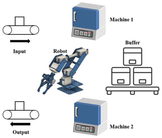
Figure 8.
A small flexible manufacturing cell.
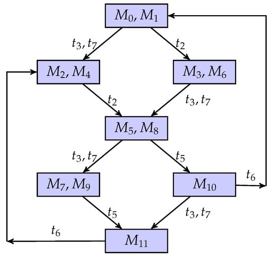
The system is modeled by Petri nets in Figure 9, where places and all transitions are unobservable. Furthermore, the meanings of all places and transitions are displayed in Table 3. A coverability graph is shown in Figure 10, where a marking of the system is denoted as . Based on the set of unobservable places, we can infer that the set of truly unobservable transitions is , and . Moreover, the mapping matrix is assumed as follows by using the technique presented, as aforementioned:
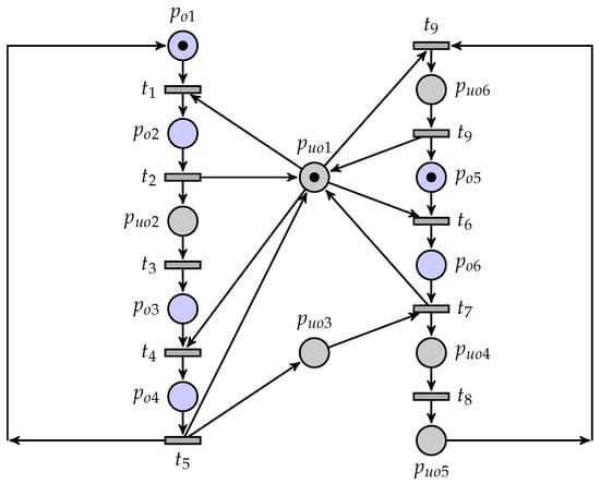
Figure 9.
The Petri net model.
Table 3.
Meaning of transitions and places.
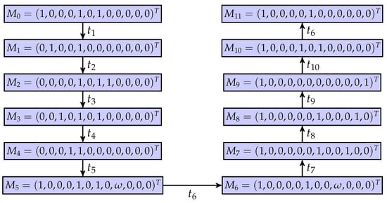
Figure 10.
A coverability graph of the net system.
Figure 11 is a BCG of the flexible manufacturing cell using the partial markings and quasi-observable transitions. The results of the current-state estimation with partial markings are shown in Figure 12. In this work, we assume that the process of Machine 2 is the confidential information of the system, i.e., the secret states are . Its BCG-based observer, as shown in Figure 13, is constructed to verify if the system is current-state opaque.
Figure 11.
A BCG of the net system.
Figure 12.
The result of state estimation.
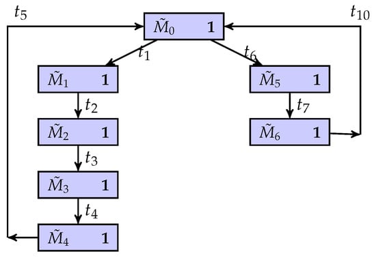
Figure 13.
The BCG-based observer.
There is a possibility that when the system is invaded by intruders, the system can keep secret information. Specifically, an intruder can infer the system’s quasi-observable transitions and build the corresponding BCG of the system. When they observe that the evolution of the system is , the corresponding partial marking of the system is , and at the same time, , and . This means that the intruder cannot determine whether the current state of the system must be a secret state. On the other hand, for other partial marks, there is no possible secret state in their current state estimation results. In other words, in the BCG-based observer of the system, the binary scalar of any node is equal to one, i.e., . Therefore, the flexible manufacturing cell is current-state opaque.
Based on this example, we can find that for a manufacturing system, because goods are constantly transported, loaded, and unloaded, a real system is in general not bounded, as it is reasonable to assume that the production is continuous without any interruption. In other words, unbounded systems are more common than bounded systems. Furthermore, the method reported in this particular research not only is successfully applied to the proposed example but also shows that this method can be closer to the conditions of unbounded systems in the real world. Therefore, this method is more effective in solving the problem of confidentiality of confidential information in the real world.
6. Conclusions
This paper deals with the verification of CSO in partially observed unbounded Petri nets, where the truly unobservable subnet is acyclic. The coverability problem and complete state estimation problem are explored by using the novel basis coverability graph. This research proves that the BCG can verify the CSO problems by constructing a BCG-based observer. This approach is characterized by the fact that the CSO problem can be accomplished based on only a few observations. Specific examples are presented and illustrate that this approach is effective.
However, based on the real-world example, one deficiency in this research is also recognized. From the viewpoint of graph theory, Petri nets are a topological structure of a real system, and their nodes correspond to the components of the system. This phenomenon leads to the necessity of reusing Petri nets for modeling if the structure of the system or topology is changed. To help system administrators analyze system performance, adaptive modeling methods developed for system structure changes will become a new research topic.
In future work, unbounded Petri nets and their basis coverability graphs are still our research interest. All the typical problems arising in the domain of discrete event systems modeled with unbounded Petri nets will be continuously explored, such as the verification of initial-state opacity and language-based opacity, the analysis of detectability [35,36], the enforcement of opacity based on supervisory control [37], and fault diagnosis and diagnosability analysis [38]. It is also interesting to address various scheduling problems of automated production systems [39] with the opacity property being guaranteed.
Author Contributions
Conceptualization, H.Z., and Z.L.; methodology, H.Z.; validation, H.Z., and Z.L.; Formal analysis, A.M.E.-S.; Resources, M.A.E.-M.; Writing—original draft, H.Z.; Writing—review & editing, Z.L.; Supervision, A.M.F.-F., and Z.L.; Project administration, A.M.E.-S., M.A.E.-M., and Z.L. All authors have read and agreed to the published version of the manuscript.
Funding
This research was funded by the Science and Technology Fund, FDCT, Macau SAR, under grant 0064/2021/A2, and by the Special Fund for Scientific and Technological Innovation Strategy of Guangdong Province under grant No. 2022A0505030025. The authors extend their appreciation to King Saud University, Saudi Arabia, for funding this work through Researchers Supporting Project number (RSP2023R133), King Saud University, Riyadh, Saudi Arabia.
Data Availability Statement
Date are contained within the article.
Conflicts of Interest
The authors declare no conflict of interest.
References
- Lin, F. Opacity of discrete event systems and its applications. Automatica 2011, 47, 496–503. [Google Scholar] [CrossRef]
- Mazaré, L. Using unification for opacity properties. In Proceedings of the 4th IFIP WGI, Baracelona, Spain, 5–7 April 2004; Volume 7, pp. 165–176. [Google Scholar]
- Jacob, R.; Lesage, J.-J.; Faure, J.-M. Overview of discrete event systems opacity: Models, Validation, and Quantification. Annu. Rev. Control 2016, 41, 135–146. [Google Scholar] [CrossRef]
- Tong, Y.; Li, Z.; Seatzu, C.; Giua, A. Verification of current-state opacity using Petri nets. In Proceedings of the American Control Conference, Chicago, IL, USA, 1–3 July 2015; pp. 1935–1940. [Google Scholar]
- Saadaoui, I.; Li, Z.; Wu, N. Current-state opacity modelling and verification in partially observed Petri nets. Automatica 2020, 116, 108907. [Google Scholar] [CrossRef]
- Tong, Y.; Li, Z.; Seatzu, C.; Giua, A. Verification of state-based opacity using Petri nets. IEEE Trans. Autom. Control 2017, 62, 2823–2837. [Google Scholar] [CrossRef]
- Tong, Y.; Li, Z.; Seatzu, C.; Giua, A. Verification of initial-state opacity in Petri nets. In Proceedings of the 54th IEEE Conference on Decision and Control, Osaka, Japan, 15–18 December 2015; pp. 344–349. [Google Scholar]
- Saboori, A.; Hadjicostis, C.N. Verification of k-step opacity and analysis of its complexity. IEEE Trans. Autom. Sci. Eng. 2011, 8, 549–559. [Google Scholar] [CrossRef]
- Falcone, Y.; Marchand, H. Runtime enforcement of k-step opacity. In Proceedings of the 52nd IEEE Conference on Decision and Control, Firenze, Italy, 10–13 December 2013; pp. 7271–7278. [Google Scholar]
- Yin, X.; Li, S. Synthesis of dynamic masks for infinite-step opacity. IEEE Trans. Autom. Control 2020, 65, 1429–1441. [Google Scholar] [CrossRef]
- Ma, Z.; Yin, X.; Li, Z. Verification and enforcement of strong infinite-step and k-step opacity using state recognizers. Automatica 2021, 133, 109838. [Google Scholar] [CrossRef]
- Paoli, A.; Lin, F. Decentralized opacity of discrete event systems. In Proceedings of the America Control Conference, Montreal, QC, Canada, 27–29 June 2012; Volume 99, pp. 6083–6088. [Google Scholar]
- Deng, W.; Yang, J.; Jiang, C.; Qiu, D. Opacity of fuzzy discrete event systems. In Proceedings of the Chinese Control and Decision Conference, Nanchang, China, 3–5 June 2019; pp. 1840–1845. [Google Scholar]
- Cong, X.; Fanti, M.; Mangini, M.; Li, Z. On-line verification of current-state opacity by Petri nets and integer linear programming. Automatica 2018, 94, 205–213. [Google Scholar] [CrossRef]
- Zhang, C.; Tian, G.; Fathollahi-Fard, A.M.; Wang, W.; Wu, P.; Li, Z. Interval-valued intuitionistic uncertain linguistic cloud Petri net and its application to Risk assessment for subway fire accident. IEEE Trans. Autom. Sci. Eng. 2022, 19, 163–177. [Google Scholar] [CrossRef]
- Cassandras, C.G.; Lafortune, S. Introduction to Discrete Event Systems, 2nd ed.; Springer Science & Business Media: New York, NY, USA, 2009. [Google Scholar]
- Zhu, G.; Feng, L.; Li, Z.; Wu, N. An efficient fault diagnosis approach based on integer linear programming for labeled Petri nets. IEEE Trans. Autom. Control 2021, 66, 2393–2398. [Google Scholar] [CrossRef]
- Cabasino, M.P.; Giua, A.; Seatzu, C. Diagnosability of bounded Petri nets. In Proceedings of the 48th IEEE Conference on Decision and Control Held Jointly with 28th Chinese Control Conference, Shanghai, China, 15–18 December 2009; pp. 1254–1260. [Google Scholar]
- Lin, F.; Wang, W.; Han, L.; Shen, B. State estimation of multichannel networked discrete event systems. IEEE Trans. Control Netw. Syst. 2020, 7, 53–63. [Google Scholar] [CrossRef]
- Ma, Z.; Tong, Y.; Li, Z.; Giua, A. Basis marking representation of Petri net reachability spaces and its application to the reachability problem. IEEE Trans. Autom. Control 2017, 62, 1078–1093. [Google Scholar] [CrossRef]
- Zhu, G.; Li, Z.; Wu, N. Model-based fault identification of discrete event systems using partially observed Petri nets. Automatica 2018, 96, 201–212. [Google Scholar] [CrossRef]
- Ushio, T.; Onishi, I.; Okuda, K. Fault detection based on Petri net models with faulty behaviors. In Proceedings of the IEEE International Conference on Systems, Man, and Cybernetics, San Diego, CA, USA, 14 October 1998; pp. 113–118. [Google Scholar]
- Cabasino, M.P.; Giua, A.; Lafortune, S.; Seatzu, C. Diagnosability analysis of unbounded Petri nets. In Proceedings of the 48th IEEE Conference on Decision and Control Held Jointly with 28th Chinese Control Conference, Shanghai, China, 15–18 December 2009; pp. 1267–1272. [Google Scholar]
- Finkel, A. The Minimal Coverability Graph for Petri Nets; Springer: Berlin/Heidelberg, Germany, 1991; pp. 210–243. [Google Scholar]
- Valmari, A.; Hansen, H. Old and new algorithms for minimal coverability sets. Fundam. Inform. 2014, 131, 1–25. [Google Scholar] [CrossRef]
- Wang, S.; Zhou, M.; Li, Z.; Wang, C. A new modified reachability tree approach and its applications to unbounded Petri nets. IEEE Trans. Syst. Man Cybern. Syst. 2013, 43, 932–940. [Google Scholar] [CrossRef]
- Lefaucheux, E.; Giua, A.; Seatzu, C. Basis coverability graph for partially observable Petri nets with application to diagnosability analysis. In Proceedings of the International Conference on Applications and Theory of Petri Nets and Concurrency, Bratislava, Slovakia, 24–29 June 2018; pp. 164–183. [Google Scholar]
- Tong, Y.; Ma, Z.; Li, Z.; Seactzu, C.; Giua, A. Verification of language-based opacity in Petri nets using verifier. In Proceedings of the American Control Conference, Boston, MA, USA, 6–8 July 2016; pp. 757–763. [Google Scholar]
- Zhu, H.; Yin, L.; Wu, N.; Li, Z. Verification of current-state opacity for discrete event systems modeled with unbounded Petri nets. In Proceedings of the 8th International Conference on Control, Decision and Information Technologies, Istanbul, Turkey, 17–20 May 2022; pp. 1261–1266. [Google Scholar]
- Bryans, J.W.; Koutny, M.; Ryan, P.Y. Modelling opacity using Petri nets. Electron. Notes Theor. Comput. Sci. 2005, 121, 101–115. [Google Scholar] [CrossRef]
- Bryans, J.W.; Koutny, M.; Mazaré, L.; Ryan, P.Y. Opacity generalised to transition systems. Int. J. Inf. Secur. 2008, 7, 421–435. [Google Scholar] [CrossRef]
- Zhu, H. Preliminaries of Petri Nets. Available online: https://github.com/Zhiwuli/Zhiwu-must/blob/master/Preliminaries%20of%20Petri%20nets.pdf (accessed on 18 January 2023).
- Cabasino, M.P.; Giua, A.; Seatzu, C. Fault detection for discrete event systems using Petri nets with unobservable transitions. Automatica 2010, 46, 1531–1539. [Google Scholar] [CrossRef]
- Lu, F.; Zeng, Q.; Zhou, M.; Bao, Y.; Duan, H. Complex reachability trees and their application to deadlock detection for unbounded Petri nets. IEEE Trans. Syst. Man Cybern. Syst. 2019, 49, 1164–1174. [Google Scholar] [CrossRef]
- Shu, S.; Lin, F.; Ying, H. Detectability of discrete event systems. IEEE Trans. Autom. Control 2007, 52, 2356–2359. [Google Scholar] [CrossRef]
- Lan, H.; Tong, Y.; Guo, J.; Seatzu, C. Verification of C-detectability using Petri nets. Inf. Sci. 2020, 528, 294–310. [Google Scholar] [CrossRef]
- Saboori, A.; Hadjicostis, C.N. Opacity-enforcing supervisory strategies via state estimator constructions. IEEE Trans. Autom. Control 2012, 57, 1155–1165. [Google Scholar] [CrossRef]
- Cabasino, M.P.; Giua, A.; Lafortune, S.; Seatzu, C. A new approach for diagnosability analysis of Petri nets using verifier nets. IEEE Trans. Autom. Control 2012, 57, 3104–3117. [Google Scholar] [CrossRef]
- Tian, Z.; Jiang, X.; Liu, W.; Li, Z. Dynamic energy-efficient scheduling of multi-variety and small batch flexible job-shop: A case study for the aerospace industry. Comput. Ind. Eng. 2023, 178, 109111. [Google Scholar] [CrossRef]


Disclaimer/Publisher’s Note: The statements, opinions and data contained in all publications are solely those of the individual author(s) and contributor(s) and not of MDPI and/or the editor(s). MDPI and/or the editor(s) disclaim responsibility for any injury to people or property resulting from any ideas, methods, instructions or products referred to in the content. |
© 2023 by the authors. Licensee MDPI, Basel, Switzerland. This article is an open access article distributed under the terms and conditions of the Creative Commons Attribution (CC BY) license (https://creativecommons.org/licenses/by/4.0/).