
Multi-Objective LQG Design with Primal-Dual Method


Abstract
1. Introduction
2. Finite-Horizon LQG Problem
- for all and ;
- , .
3. Main Results
3.1. Lagrangian Solution
- Primal feasibility condition:
- Complementary slackness condition:
- Dual feasibility condition:
- Stationary condition :where .
- If the strict inequality is already satisfied with obtained using the standard Riccati equation, then solves the complementary slackness condition. We do not need to do anything in this case.
- Moreover, if the equality is satisfied with obtained using the standard Riccati equation, then any solves the complementary slackness condition. However, when , the corresponding may be different from . Therefore, to use the variables obtained in Proposition 1 as a solution to the KKT condition, we need to set .
- Lastly, assume that holds with obtained using the standard Riccati equation. Then, some solves the complementary slackness condition if . Suppose that is such a number. Then, the corresponding tuple satisfies the KKT condition.
- 1.
- f is continuous over ;
- 2.
- holds for any ;
- 3.
- If holds for some , then ;
- 4.
- ;
- 5.
- There exists a such that ;
- 6.
- Define the set-valued mapping . Then, is a closed line segment.
- From the definition, is linear in , is rational, whose entries are finite for a finite because the inverse matrix in is finite for all . Therefore, from the definition, is also rational and finite over , which implies that is continuous in . This completes the proof.
- We only need to prove the inequality for . By contradiction, suppose that holds. For a fixed , we see from the KKT condition that the problem is nothing but the optimizationwith an augmented objective. Since is the optimal solution corresponding to , it follows thatwhere is the optimal solution corresponding to . On the other hand, we havewhich leads to
- The fourth statement is true due to Assumption 3.
- Note that the objective in (13) can be replaced with without changing the optimal solutions. As , the objective converges to , which implies as due to the strict feasibility assumption in Assumption 2. Since f is continuous over from the first statement, there should exists such that .
- Define and . From the continuity of f, the supremum and infimum are attained; otherwise, f should be discontinuous. Therefore, we can define and . From the second statement, we see that for all . It completes the proof.
3.2. Algorithm
| Algorithm 1 Primal-Dual Method with Bisection Line Search. |
|
| Algorithm 2 Policy evaluation . |
|
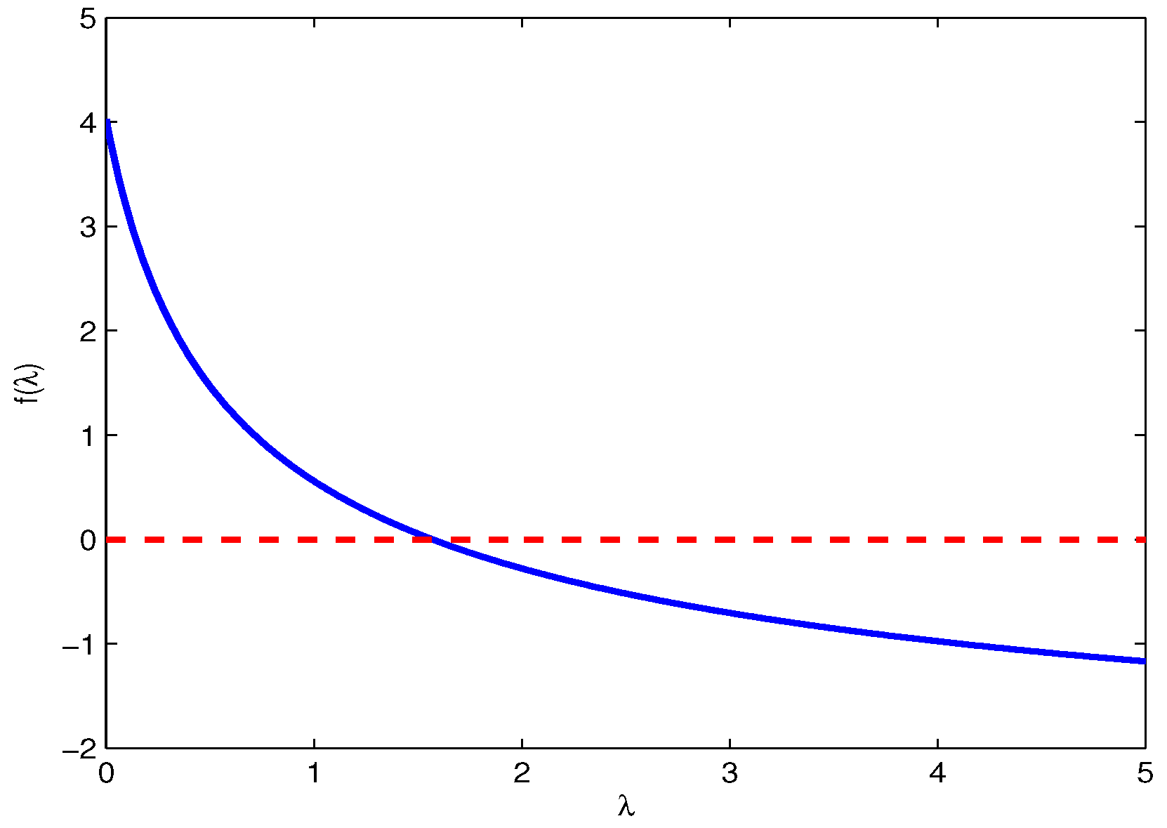
3.3. Suboptimality
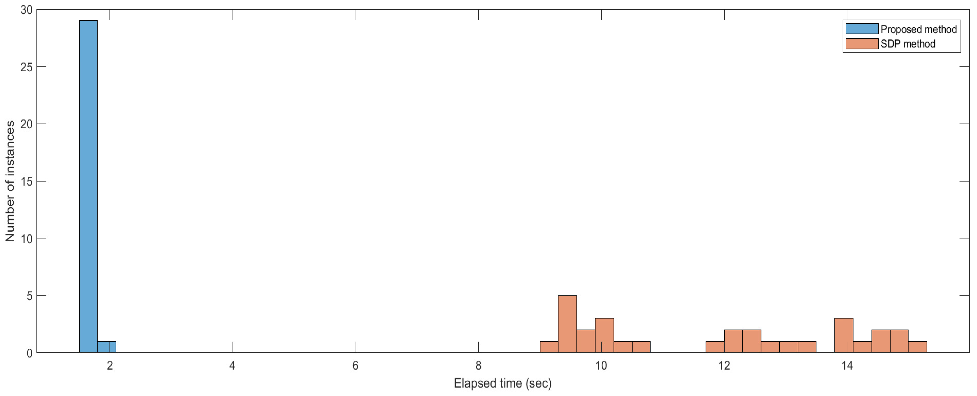
3.4. Computational Efficiency
3.5. Deterministic Cases
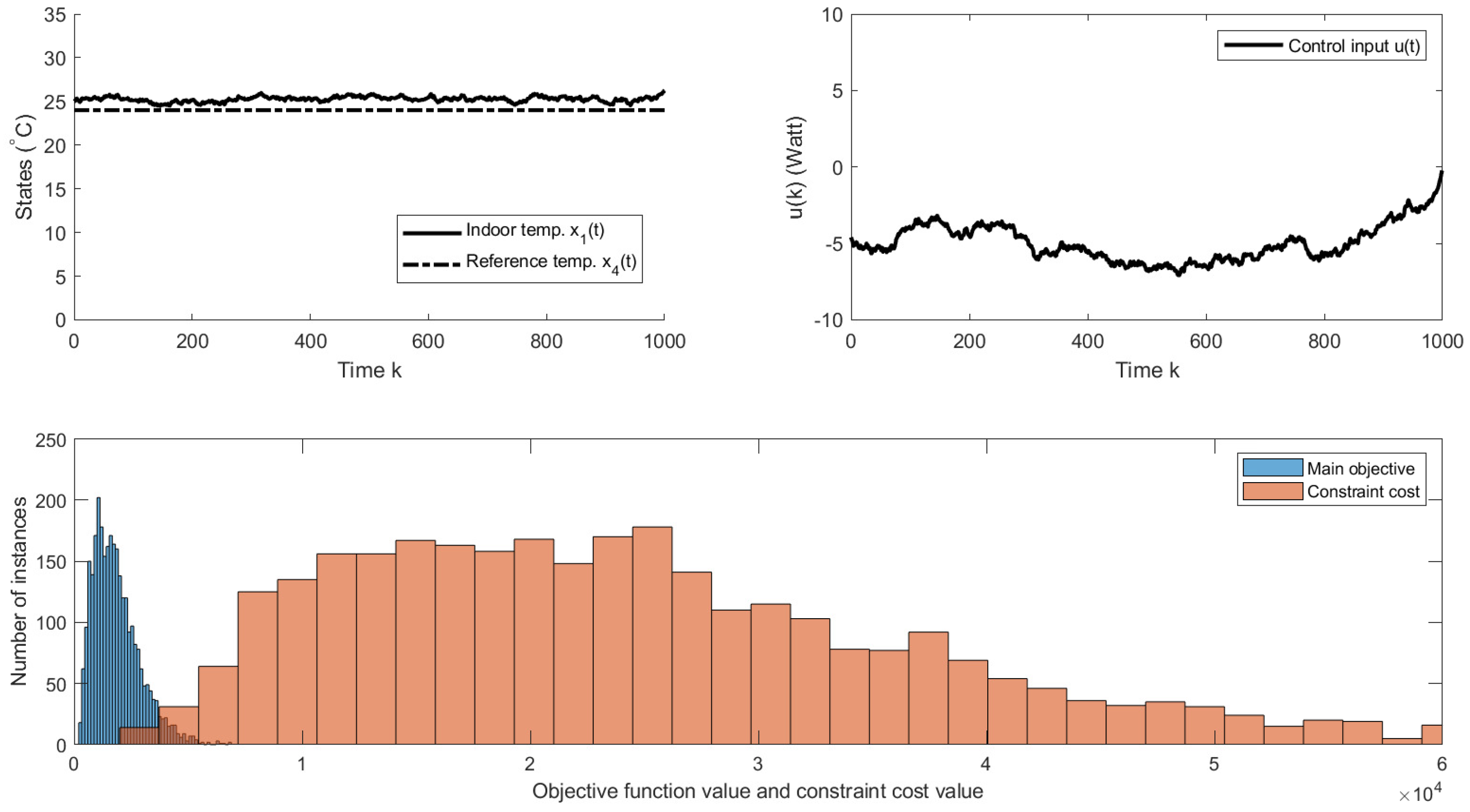
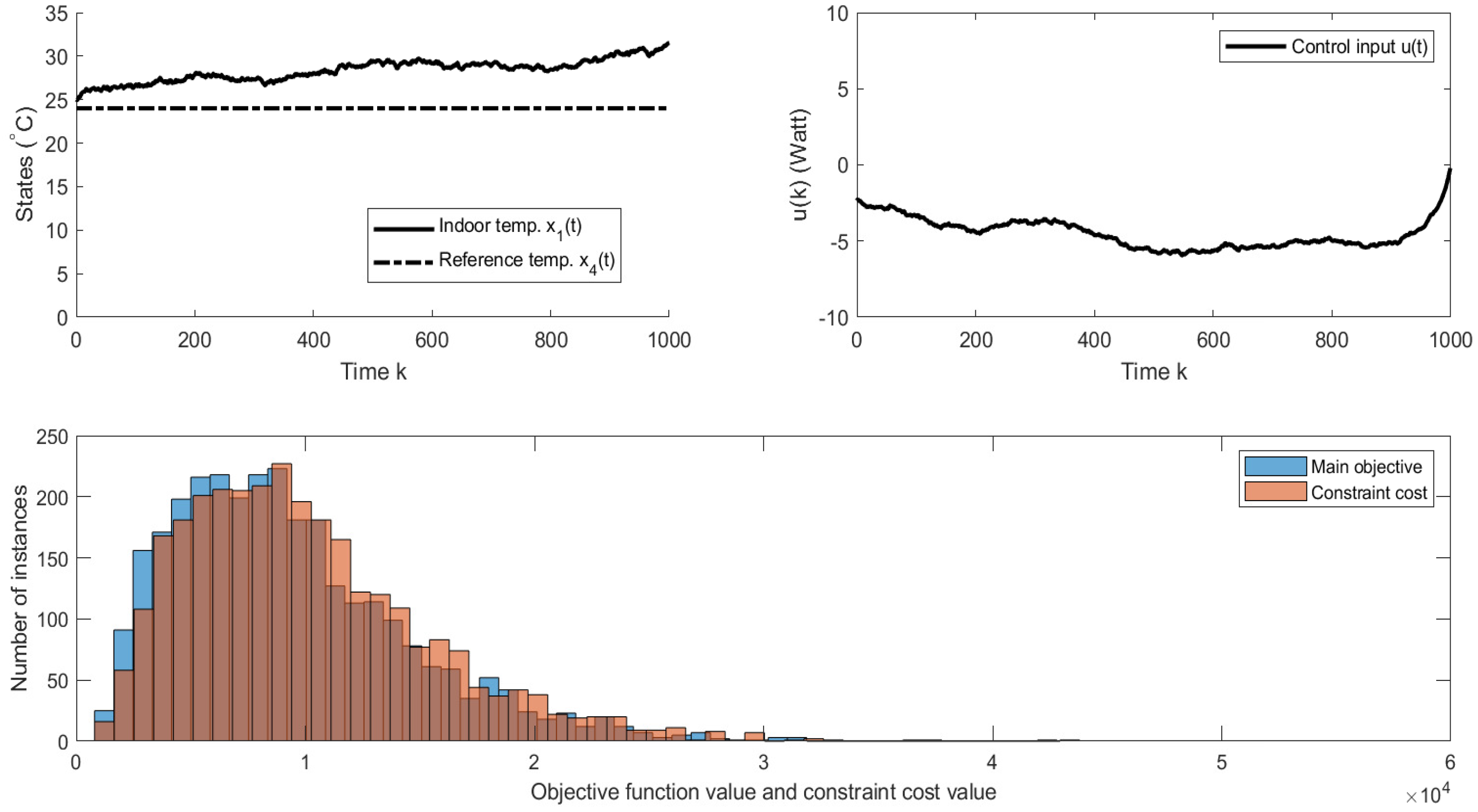
3.6. Example
4. Conclusions
Funding
Conflicts of Interest
References
- Bertsekas, D.P.; Tsitsiklis, J.N. Neuro-Dynamic Programming; Athena Scientific: Belmont, MA, USA, 1996. [Google Scholar]
- Bertsekas, D.P. Dynamic Programming and Optimal Control, 3rd ed.; Athena Scientific: Nashua, MA, USA, 2005; Volume 1. [Google Scholar]
- Lee, D. Convergence of Dynamic Programming on the Semidefinite Cone for Discrete-Time Infinite-Horizon LQR. IEEE Trans. Autom. Control 2022, 67, 5661–5668. [Google Scholar] [CrossRef]
- Sabermahani, S.; Ordokhani, Y. Fibonacci wavelets and Galerkin method to investigate fractional optimal control problems with bibliometric analysis. J. Vib. Control 2021, 27, 1778–1792. [Google Scholar] [CrossRef]
- Boyd, S.; Vandenberghe, L. Convex Optimization; Cambridge University Press: Cambridge, UK, 2004. [Google Scholar]
- Vandenberghe, L.; Boyd, S. Semidefinite programming. SIAM Rev. 1996, 38, 49–95. [Google Scholar] [CrossRef]
- Boyd, S.; El Ghaoui, L.; Feron, E.; Balakrishnan, V. Linear Matrix Inequalities in Systems and Control Theory; SIAM: Philadelphia, PA, USA, 1994. [Google Scholar]
- El Ghaoui, L.; Niculescu, S.I. Advances in Linear Matrix Inequality Methods in Control; SIAM: University City, PA, USA, 2000; Volume 2. [Google Scholar]
- Scherer, C.; Weiland, S. Linear Matrix Inequalities in Control; Lecture Notes; Dutch Institute for Systems and Control: Delft, The Netherlands, 2000; Volume 3. [Google Scholar]
- Lee, D.H.; Park, J.B.; Joo, Y.H. A less conservative LMI condition for robust D-stability of polynomial matrix polytopes—A projection approach. IEEE Trans. Autom. Control 2010, 56, 868–873. [Google Scholar] [CrossRef]
- Lee, D.H.; Joo, Y.H. A note on sampled-data stabilization of LTI systems with aperiodic sampling. IEEE Trans. Autom. Control 2015, 60, 2746–2751. [Google Scholar] [CrossRef]
- Cao, Y.Y.; Lin, Z. A descriptor system approach to robust stability analysis and controller synthesis. IEEE Trans. Autom. Control 2004, 49, 2081–2084. [Google Scholar] [CrossRef]
- Oliveira, R.C.; Peres, P.L. Parameter-dependent LMIs in robust analysis: Characterization of homogeneous polynomially parameter-dependent solutions via LMI relaxations. IEEE Trans. Autom. Control 2007, 52, 1334–1340. [Google Scholar] [CrossRef]
- Ramos, D.C.; Peres, P.L. An LMI condition for the robust stability of uncertain continuous-time linear systems. IEEE Trans. Autom. Control 2002, 47, 675–678. [Google Scholar] [CrossRef]
- Chesi, G.; Garulli, A.; Tesi, A.; Vicino, A. Polynomially parameter-dependent Lyapunov functions for robust stability of polytopic systems: An LMI approach. IEEE Trans. Autom. Control 2005, 50, 365–370. [Google Scholar] [CrossRef]
- Fridman, E.; Shaked, U. Parameter dependent stability and stabilization of uncertain time-delay systems. IEEE Trans. Autom. Control 2003, 48, 861–866. [Google Scholar] [CrossRef]
- Yan, S.; Shen, M.; Nguang, S.K.; Zhang, G. Event-triggered H∞ control of networked control systems with distributed transmission delay. IEEE Trans. Autom. Control 2019, 65, 4295–4301. [Google Scholar] [CrossRef]
- Felipe, A.; Oliveira, R.C. An LMI-based algorithm to compute robust stabilizing feedback gains directly as optimization variables. IEEE Trans. Autom. Control 2020, 66, 4365–4370. [Google Scholar] [CrossRef]
- Guo, M.; De Persis, C.; Tesi, P. Data-driven stabilization of nonlinear polynomial systems with noisy data. IEEE Trans. Autom. Control 2021, 67, 4210–4217. [Google Scholar] [CrossRef]
- Lee, D.; Lee, S.; Karava, P.; Hu, J. Simulation-based policy gradient and its building control application. In Proceedings of the 2018 Annual American Control Conference (ACC), Milwaukee, WI, USA, 27–29 June 2018; pp. 5424–5429. [Google Scholar]
- Ma, Y.; Borrelli, F. Fast stochastic predictive control for building temperature regulation. In Proceedings of the 2012 American Control Conference (ACC), Montreal, QC, Canada, 27–29 June 2012; pp. 3075–3080. [Google Scholar]
- Oldewurtel, F.; Parisio, A.; Jones, C.N.; Morari, M.; Gyalistras, D.; Gwerder, M.; Stauch, V.; Lehmann, B.; Wirth, K. Energy efficient building climate control using stochastic model predictive control and weather predictions. In Proceedings of the 2010 American Control Conference, Baltimore, ML, USA, 30 June–2 July 2010; pp. 5100–5105. [Google Scholar]
- Luenberger, D.G.; Ye, Y. Linear and Nonlinear Programming; Addison-Wesley: Reading, MA, USA, 1984; Volume 2. [Google Scholar]
- Bemporad, A.; Morari, M.; Dua, V.; Pistikopoulos, E.N. The explicit linear quadratic regulator for constrained systems. Automatica 2002, 38, 3–20. [Google Scholar] [CrossRef]
- Grieder, P.; Borrelli, F.; Torrisi, F.; Morari, M. Computation of the constrained infinite time linear quadratic regulator. Automatica 2004, 40, 701–708. [Google Scholar] [CrossRef]
- Borrelli, F. Constrained Optimal Control of Linear and Hybrid Systems; Springer: Berlin/Heidelberg, Germany, 2003; Volume 290. [Google Scholar]
- Chisci, L.; Zappa, G. Fast algorithm for a constrained infinite horizon LQ problem. Int. J. Control 1999, 72, 1020–1026. [Google Scholar] [CrossRef]
- Rotea, M.A. The generalized H2 control problem. Automatica 1993, 29, 373–385. [Google Scholar] [CrossRef]
- Gattami, A. Generalized linear quadratic control. IEEE Trans. Autom. Control 2010, 55, 131–136. [Google Scholar] [CrossRef]
- Kothare, M.V.; Balakrishnan, V.; Morari, M. Robust constrained model predictive control using linear matrix inequalities. Automatica 1996, 32, 1361–1379. [Google Scholar] [CrossRef]
- Primbs, J.A.; Sung, C.H. Stochastic receding horizon control of constrained linear systems with state and control multiplicative noise. IEEE Trans. Autom. Control 2009, 54, 221–230. [Google Scholar] [CrossRef]
- Costa, O.L.V.; Assumpção Filho, E.; Boukas, E.; Marques, R. Constrained quadratic state feedback control of discrete-time Markovian jump linear systems. Automatica 1999, 35, 617–626. [Google Scholar] [CrossRef]
- Gahinet, P.; Nemirovski, A.; Laub, A.J.; Chilali, M. LMI Control Toolbox; The Math Works Inc.: Natick, MA, USA, 1996. [Google Scholar]
- Sturm, J.F. Using SeDuMi 1.02, a MATLAB toolbox for optimization over symmetric cones. Optim. Methods Softw. 1999, 11, 625–653. [Google Scholar] [CrossRef]
- Lofberg, J. YALMIP: A toolbox for modeling and optimization in MATLAB. In Proceedings of the 2004 IEEE International Conference on Robotics and Automation (IEEE Cat. No. 04CH37508), New Orleans, LA, USA, 2–4 September 2004; pp. 284–289. [Google Scholar]


Disclaimer/Publisher’s Note: The statements, opinions and data contained in all publications are solely those of the individual author(s) and contributor(s) and not of MDPI and/or the editor(s). MDPI and/or the editor(s) disclaim responsibility for any injury to people or property resulting from any ideas, methods, instructions or products referred to in the content. |
© 2023 by the author. Licensee MDPI, Basel, Switzerland. This article is an open access article distributed under the terms and conditions of the Creative Commons Attribution (CC BY) license (https://creativecommons.org/licenses/by/4.0/).
Share and Cite
Lee, D. Multi-Objective LQG Design with Primal-Dual Method. Mathematics 2023, 11, 1857. https://doi.org/10.3390/math11081857
Lee D. Multi-Objective LQG Design with Primal-Dual Method. Mathematics. 2023; 11(8):1857. https://doi.org/10.3390/math11081857
Chicago/Turabian StyleLee, Donghwan. 2023. "Multi-Objective LQG Design with Primal-Dual Method" Mathematics 11, no. 8: 1857. https://doi.org/10.3390/math11081857
APA StyleLee, D. (2023). Multi-Objective LQG Design with Primal-Dual Method. Mathematics, 11(8), 1857. https://doi.org/10.3390/math11081857