POFCM: A Parallel Fuzzy Clustering Algorithm for Large Datasets

Abstract

Clustering algorithms have proven to be a useful tool to extract knowledge and support decision making by processing large volumes of data. Hard and fuzzy clustering algorithms have been used successfully to identify patterns and trends in many areas, such as finance, healthcare, and marketing. However, these algorithms significantly increase their solution time as the size of the datasets to be solved increase, making their use unfeasible. In this sense, the parallel processing of algorithms has proven to be an efficient alternative to reduce their solution time. It has been established that the parallel implementation of algorithms requires its redesign to optimise the hardware resources of the platform that will be used. In this article, we propose a new parallel implementation of the Hybrid OK-Means Fuzzy C-Means (HOFCM) algorithm, which is an efficient variant of Fuzzy C-Means, in OpenMP. An advantage of using OpenMP is its scalability. The efficiency of the implementation is compared against the HOFCM algorithm. The experimental results of processing large real and synthetic datasets show that our implementation tends to more efficiently solve instances with a large number of clusters and dimensions. Additionally, the implementation shows excellent results concerning speedup and parallel efficiency metrics. Our main contribution is a Fuzzy clustering algorithm for large datasets that is scalable and not limited to a specific domain.

1. Introduction

In recent years, technological developments have caused an exponential increase in data generation and storage. According to the latest estimates, the volume of data generated by private and public institutions worldwide is expected to exceed 180 zettabytes by 2025 [1]. One of the ways to acquire new knowledge from these large amounts of data is through clustering algorithms. In this sense, a detailed analysis of these data could extract valuable information and allow better decisions to be made [2,3].

Clustering aims to partition a set of n objects in subsets, called clusters, in such a way that objects in any cluster have similar attributes and, at the same time, are different from objects in any other cluster [4]. Clustering has been extensively studied in many areas, such as data mining, pattern recognition, business management, and image processing [5,6].

Traditionally, clustering algorithms have been divided into hierarchical and partitional [7]. In turn, partitional algorithms have been divided into hard and fuzzy. The most widely used hard clustering algorithm is K-Means [8]. Hard partitional clustering algorithms constrain each object in the dataset to belong to exactly one cluster. However, there are problems in which it is desirable to represent objects with different degrees of membership [9,10]. This requirement has led to the development of fuzzy clustering algorithms. The most widely used fuzzy clustering algorithm is the Fuzzy C-Means algorithm (FCM) [11,12]. A disadvantage of FCM concerning K-Means is its computational complexity. In [13], the time complexity of the FCM algorithm is O(ndc²r), where n is the number of objects, d is the number of dimensions or attributes, c is the number of clusters, and r is the number of iterations.

Clustering is one of the most studied NP-hard problems in the scientific community [14]. To date, it is not known whether there are efficient algorithms to solve large datasets in polynomial time. These problems are considered computationally intractable. Therefore, improving the FCM clustering algorithm is a relevant and open research problem.

In the specialized literature, at least four types of improvements to the standard FCM algorithm have been found: (a) those oriented to a specific domain [15,16]; (b) improvements in one phase of the algorithm [17]; (c) those with a hybrid approach [18,19,20]; (d) those with a parallel approach. Regarding the last one, the FCM algorithm has been parallelised using different platforms and architectures, for example, Message Passing Interface (MPI) [21], cloud-based [22,23], GPU [24,25,26,27,28,29,30], Spark [31,32], Map Reduce [22,33,34,35], OpenCL [36], and OpenMP [37,38].

In contrast, our proposal is independent of the application domain; it is designed to solve large datasets, such as Big Data. In particular, our algorithm is inspired by a highly efficient sequential variant called HOFCM [20]. This variant was experimentally validated with real and synthetic datasets, and its results were contrasted with those of other sequential algorithms, such as FCM++ [17], FCM-K-Means [18], and NFCM [19], obtaining generally better results [20]. In particular, the HOFCM experimental results presented in [20] showed a solution time reduction of up to 93.94% compared to standard FCM and a solution quality reduction of 2.51% in the worst case. In this sense, our improvement proposal, which we call Parallel Optimisation Fuzzy C-Means (POFCM), significantly reduces HOFCM’s solution time. For example, values for the speedup indicators of 3.96 and a parallel efficiency of 0.99 were obtained. We use a hybrid approach that integrates K++ algorithms, O-K-Means, and the standard FCM [39]. A parallel implementation is proposed through the OpenMP multiprocessing technique. The main contributions of this paper include the following:

1.

A parallel version of an optimised variant of the FCM clustering algorithm.

2.

The detailed implementation of the FCM algorithm with the OpenMP parallelisation technique.

3.

The parallel version is discussed and evaluated, in particular, regarding the speedup and parallel efficiency metrics.

4.

Our solution approach is scalable to platforms with higher hardware capabilities and is not limited to solving domain-specific datasets.

This paper is organised as follows: Section 2 describes the related works. Section 3 introduces the clustering algorithms used. Section 4 presents the improvement proposal. Section 5 presents the performance and evaluation under different scenarios. Section 6 reports the results obtained. Conclusions and ideas for future research are provided in Section 7.

2. Related Work

Clustering algorithms have been extensively studied. However, there are few works on parallel implementations of the FCM algorithm with the OpenMP technique. This section describes other parallel implementations of the FCM algorithm to contrast our solution approach and results.

Table 1. Comparison of recent parallel FCM clustering algorithms.

Algorithm	P	D	Platforms	I	H	Equipment Features	Largest Dataset (Objects × Attributes)	Type	Sec. FCM	Others	Variant Sec.
DFCM DOFCM DKFCM [22]		✓	Cloud base Map Reduce	✓	✓	20 machines, Intel® Core™ i7 3.2 GHz, 8 GB RAM, 2 TB Hard drive	(30,000,000,000 × 150)	2 R	✓	✓
DFCM [23]		✓	Cloud base			-----	(1024 × 10)	1 R	✓	✓
PFMGPU [21]	✓		GPU-MPI			Intel® Core™ i7 3.4 GHz, 16 GB RAM, GPU NVidia GeForce GTS 450 with 4 SMs	(40,646 × 2)	2 R 1 S		✓	✓
brFCM [24]	✓		GPU	✓		Intel® Core™ i5 Compiler GCC 4.7, Ubuntu OS, Tesla M2070 y Tesla K20m	262,144 pixels	2 R	✓
PBCFCM1 PBCFCM2 [25]	✓		GPU		✓	Intel® Core™ i5-3230M, 2.6 GHz, NVidia GeForce GT 740m, 2 GB GPU	7,929,856 pixels	4 R			✓
DP/HCG/ HNP [26]	✓		GPU		✓	Intel® Core™ i7, 8 GB RAM, NVidia GeForce GT 840M, Windows 8	-----	2 R	✓		✓
PFCM [27]	✓		GPU			Intel® Core™ i7 32 GB RAM, NVidia GTX 970 6 GB	-----	1 R	✓
K-Means FM/FCM [28]	✓		GPU			Intel Xeon® Silver 4216, 3.20 GHz, Nvidia RTX 2080 Ti	(100,000 × 80)	1 S	✓	✓
FM FCM GK-FCM [29]	✓		GPU			Intel® Skylake-X™ i7-37820X, 3.60 GHz. Nvidia A100, 2.4 GHz Nvidia V100, 2.7 GHz	(800,000 × 104)	1 S	✓	✓
PIT2FCM_1 [30]	✓		GPU		✓	Intel® Core™ i5-3230M, 2 cores, 2.6 GHz, Nvidia GeForce GT 740 m 2 GB	1,331,200 pixels	9 R			✓
PFCM [31]	✓		Spark			Intel® Xeon™ E7-4820 2.00 GHz, 8 GB RAM, 600 GB Hard Disk	2.5 GB	6 R
FCM-Ck [32]	✓		Spark	✓	✓	Intel® Core™ i5-8400, 16 GB RAM, 2 TB Hard Disk, Windows 7	(400,000 × 42)	3 R	✓	✓
ICFCM [33]	✓		Map Reduce	✓	✓	CPU 2.40 GHz, 2 GB RAM, Ubuntu 14.10	-----		✓	✓
HCFCM [34]	✓		Map Reduce	✓	✓	CPU 2.2 GHz, 4 GB RAM, 500 GB Hard Disk, Ubuntu 12.10	(1728 × 4)	2 R	✓
FCM [35]	✓		Map Reduce	✓		AMD, 8 GB RAM, 500 GB Hard Disk, Ubuntu 18.04 OS	1 GB	6 S	✓
FPGA [36]	✓		OpenCL			Intel® Core™ i7-6700 3.4 GHz, 16 GB RAM	(100,000 × 2)	1 R 3 S	✓
FCM [37]	✓		OpenMP			Intel Core 2	241,200 pixels	1 R	✓
PHFCM [38]	✓		OpenMP			Intel® Core™ i7-4510U con 4 cores, 2.00 GHz, 8 GB RAM	2,073,600 pixels	4 R		✓
POFCM	✓		OpenMP	✓		Intel® Core™ i5-4570, 4 cores, 3.30 GHz, 14 GB RAM, and 512 GB HDD, Windows 10, Compiler MSVC 2020	(40,000 × 40)	3 R 16 S			✓

provides information on different implementations of variants of FCM using different platforms and architectures. The first column shows the proposed algorithms, including the paper where they were first mentioned. The second column indicates if the implementation of the algorithm is parallel, and the third column indicates if it is distributed. The fourth column mentions the platform on which the algorithm was implemented. The fifth column indicates whether the proposed improvement was implemented in the initialisation phase of FCM. The sixth column indicates whether the proposed algorithm is hybrid. The seventh column mentions the main characteristics of the equipment used during the experimentation. The eighth column describes the largest dataset used in the experiments; in general, the number of objects is mentioned before the x, and the number of attributes or dimensions of the dataset is mentioned next; some authors express the size of the dataset in pixels or in GB. The ninth column lists the number of test datasets first, followed by an R if the dataset is real or an S if it is synthetic. The last three columns on the right indicate how the authors of each paper compare their results to assess their contribution quantitatively. The tenth column indicates if the performance was compared with the sequential FCM algorithm. The eleventh column indicates whether the comparison was made with other algorithms proposed by other authors. Finally, the twelfth column indicates whether the comparison was made in a sequential version of the parallelised algorithm.

Based on the data in Table 1, the following observations can be made:

(a)

There are few implementations in the OpenMP platform, and these correspond to recently published research. One of the most used platforms is GPU.

(b)

The FCM algorithm is sensitive to the values of the initial parameters; it is known that appropriate values can reduce the number of iterations of the algorithm. In this sense, our work proposes a hybrid improvement in the initialisation phase. As shown in column three, other authors also propose improvements in the initialisation phase.

(c)

As shown in Table 1, the hybrid improvement approach has been used in various works.

(d)

Regarding hardware, it was observed that Intel 5 and 7 processors, which are normally used in desktop computers and laptops, are predominant. Regarding the use of RAM memory, it is shown that RAM ranges between 2 and 16 GB. In addition, most hard drives range in capacity from 512 GB to 2 TB.

(e)

An important aspect of the experimentation is the characteristics of the datasets. The datasets are in the size range from 1024 to 400,000 objects. In the case of the distributed architectures, some datasets are 30,000,000,000 objects in size. In some research, the dataset size is expressed in different units, such as pixels or GB.

(f)

Three investigations that experimented with real and synthetic datasets, including ours, were identified. Most of the works only carried out experimentation using real datasets.

(g)

In our research, like four other studies, the increase in efficiency is calculated based on the performance of the parallelised algorithm in its sequential version, as shown in column 12. In most investigations, the comparison is made with the sequential version of FCM, as indicated in column 10. Six published studies are compared with variants proposed by other authors, as seen in column 11.

It is important to highlight two limitations of the improvements to the FCM algorithm with a parallel approach using the OpenMP technique. The first limitation is that they are designed to solve problems in a specific domain, such as image segmentation [37,38]. The second limitation is that the acceleration and parallel efficiency values are not shown [38].

3. Clustering Algorithms

Our proposed solution consists in parallelising the HOFCM algorithm [20], which integrates the K++, O-K-Means, and standard FCM algorithms. In this section, the K++, O-K-Means, FCM, and HOFCM algorithms are described.

3.1. K++ Algorithm

The K++ algorithm, proposed in [40], initialises the clustering centroids of the K-Means algorithm by selecting objects from the dataset that are the farthest from each other in a probabilistic manner. The pseudocode of the K++ algorithm is shown in Algorithm 1.

Algorithm 1: K++
1	Initialisation:
2	X: = {x1, …, xn};
3	Assign the value for k;
4	V: = Ø;//The set of centroids is initialised
5	V: = V U {v1};//Select the first centroid v1 randomly
6	For i = 2 to k:
7	Select the i-th centroid vi ϵ X with probability D(xi, vj)/∑xϵX D(xi, vj);
8	V: = V U {vi};
9	Endfor
10	Return V;
11	End of algorithm

In Algorithm 1, the initialisation of the centroids by the K++ algorithm is shown. Given the dataset X and the value of k, the next step is to select the first centroid k₁ in a uniform random manner from dataset X. Subsequently, it should be incorporated to the set of centroids labelled as V. For the second centroid, and until the number of centroids equals k, the i-th centroid should be selected according to a probability distribution.

3.2. O-K-Means Algorithm

In [41], O-K-Means is proposed, which accelerates the convergence process by stopping the algorithm when the total number of objects that change cluster membership in one iteration is less than a threshold. This value expresses a relationship between the computational effort and the quality of the solution. The pseudocode of the O-K-Means algorithm is shown in Algorithm 2.

Algorithm 2: O-K-Means
1	Initialisation:
2	X: = {x1, …, xn};
3	V: = {v1, …, vk};
4	εok: = Threshold value for determining O-K-Means convergence;
5	Classification:
6	For xi ϵ X and vk ϵ V{
7	Calculate the Euclidean distance from each xi to the k centroids;
8	Assign the xi object to the nearest vk centroid;
9	Compute $\gamma$};
10	Calculate centroids:
11	Calculate the centroid vk;
12	Convergence:
13	If ($\gamma$≤ εok):
14	Stop the algorithm;
15	Otherwise:
16	Go to Classification
17	End of algorithm

The indicator $\gamma$ represents the percentage of objects that change cluster membership in an iteration t, which is calculated as ${\gamma }_t$ = 100(o_t/n), where o_t is the number of objects that change cluster membership.

3.3. FCM Algorithm

The basic idea is that X = {x₁, …, x_n} is the set of n objects to be partitioned according to a similarity criterion, where x_i $\in$ R^d for i = 1, …, n; c is the number of clusters, where 2 ≤ c < n.

The fuzzy clustering problem was formulated as an optimisation problem [42], minimising a function, as shown in Equation (1).

$$P:\mathrm{minimize}{J}_m(U,V)={\displaystyle \sum _{i=1}^n}{\displaystyle \sum _{j=1}^c}{({\mu }_{ij})}^m\parallel x_i,v_j{\parallel }^2$$

(1)

where U = µ_ij is the membership matrix of each object i to each cluster j; V = {v₁, …, v_c} is the set of centroids, where v_j is the centroid of cluster j; m is the weighting exponent or the fuzzy factor that expresses how much the clusters overlap, m > 1; $\parallel x_i,v_j\parallel$² indicates the Euclidean distance between the object x_i and the centroid v_j for i = 1, …, n and j = 1, …, c.

Minimising J_m, which is an estimated model of V and U, is obtained as

$$v_j=\frac{{\displaystyle \sum _{i=1}^n{(u_{ij})}^m{x}_i}}{{\displaystyle \sum _{i=1}^n{(u_{ij})}^m}}{{{\displaystyle }}^{}}^{{}^{}}1\le j\le c$$

(2)

$$u_{ij}=\frac{1}{{\displaystyle \sum _{k=1}^c}{\left(\frac{\parallel x_i,v_j{\parallel }^2}{\parallel x_i,v_k{\parallel }^2}\right)}^{\frac{1}{m-1}}}\hspace{1em}\hspace{1em}1\le i\le n{;}^{}{}^{}1\le j\le c$$

(3)

where x_i and v_j are vectors that belong to a space R^d and are defined as follows

$$x_i=(x_1,x_2,\dots ,x_d),1\le i\le n$$

(4)

$$v_j=(v_1,v_2,\dots ,v_d),1\le j\le c$$

(5)

The constraints of fuzzy clustering are formalised in Equations (6)–(8).

$$u_{ij}\in [0,1],\hspace{1em}1\le j\le c,\hspace{1em}1\le i\le n$$

(6)

$${\displaystyle \sum _{j=1}^c{u}_{ij}=1,\hspace{1em}1\le i\le n}$$

(7)

$$0<{\displaystyle \sum _{i=1}^n{u}_{ij}<n,\hspace{1em}1\le j\le c}$$

(8)

Equation (6) indicates that the degree of membership of an object i to a cluster j must be between 0 and 1. Equation (7) declares that the sum of the degrees of membership of an object i to different clusters as necessarily being equal to 1. Equation (8) indicates that the sum of all the degrees of membership in a cluster must be greater than 0 and less than n, i.e., there must be no empty clusters and not only one cluster.

The pseudocode of the standard FCM algorithm is shown in Algorithm 3.

Algorithm 3: Standard FCM
Input: dataset X, c, m, ε
Output: V, U
1	Initialisation:
2	t: = 0;
3	U(t): = {µ11, …, µij}; is randomly generated
4	Calculate centroids:
5	Calculate the centroids using Equation (2);
6	Classification:
7	Update and calculate the membership matrix using Equation (3);
8	Convergence:
9	If max [abs(µij(t) − µij(t+1))] < ε:
10	Stop the algorithm;
11	Otherwise:
12	U(t): = U(t+1) and t: = t + 1;
13	Go to Calculate centroids
14	End of algorithm

3.4. HOFCM Algorithm

The HOFCM algorithm proposed in [20] optimises the values of the membership matrix parameter. This approach consists of three steps: (a) generate a set of n solutions of an x dataset, applying two variants of the K-Means algorithm, named K++ and O-K-Means [41]; (b) select the best solution as the basis for generating the optimised membership matrix; (c) solve the dataset X using Fuzzy C-Means. The pseudocode of the HOFCM algorithm is shown in Algorithm 4.

Algorithm 4: HOFCM
Input: dataset X, c, m, ε, εok
Output: V, U
1	Initialisation:
2	i: = 1;
3	Repeat
4	Function K++ (X, c):
5	Return V′;
6	Function O-K-Means (X, V′, εok, c):
7	Return V″;
8	i = i + 1;
9	While i <= 10;
10	Select V″ for the value of i at which the objective function obtained the minimum value;
11	Transformation function s;
12	r: = 1;
13	Calculate centroids:
14	Calculate the centroids using Equation (2);
15	Classification:
16	Update and calculate the membership matrix using Equation (3);
17	Convergence:
18	If max [abs(µij(r) − µij(r+1))] < ε:
19	Stop the algorithm;
20	Otherwise:
21	U(r): = U(r+1) and r: = r + 1;
22	Go to Calculate centroids
23	End of algorithm

The HOFCM algorithm has four phases. The first is the initialisation phase; in this phase, three functions are created: (1) The K++ function, which receives the dataset X and the number of clusters as input parameters; this function returns a set of centroids identified by variable V′. (2) The O-K-Means function, which receives dataset X, the set of centroids V′ generated from K++, and the threshold value εok as input parameters to determine the convergence of the algorithm and the number of clusters; at the end of the phase of convergence, it returns optimised centroids denoted by variable V″. (3) The transformation function s, which allows the final centroids of the O-K-Means algorithm to be transformed, taken from the lowest value of the objective function into the initial optimised values of the membership matrix; these are the input parameters for the FCM algorithm. The second, third, and fourth phases of the HOFCM algorithm, called the calculation of centroids, classification, and convergence, respectively, are typical of the standard FCM.

4. Proposal for Improvement

This section is divided into two subsections. Section 4.1 describes the parallelisation technique and shows a short program code using a directive called a pragma, and Section 4.2 describes our proposed POFCM algorithm.

4.1. OpenMP Parallelisation Technique

In this research, the new parallel hybrid algorithm POFCM is proposed. This algorithm is inspired by the HOFCM algorithm. For the parallel implementation of the algorithm, the OpenMP technique is used [43,44]. This technique has an application programming interface (API), which allows the coding of applications using parallel programming with shared memory. The programming languages that have this API are C, C++, and Fortran. The OpenMP technique allows the execution of the instruction set of each loop iteration to be parallelised, linking the execution of each iteration set to a thread (fork). One restriction is that the calculations in each iteration must be independent of the calculations in other iterations. The distribution of the calculations of each set of iterations among the threads reduces the total processing time. In this way, the OpenMP approach is scalable, as OpenMP transparently distributes the iterations among the number of threads available to the machine where the program is executed. In OpenMP, compilation directives are called pragmas. The pragma directive parallelises the set of instructions in a loop. To better understand the pragma directive, in Program 1, an example of code in C language is shown and extracted from [45]. Line 1 starts the average function, which obtains the average value of two successive items of vector a and assigns it to an item of vector b. In line 2, values are assigned to each of the items of vector a. In line 3, the pragma directive parallelises the execution of the instructions of each of the iterations of the for loop of line 4. The pragma directive assigns a block or set of iterations to each thread. This way, if the machine has three threads, thread one will process iterations 1, 2, and 3; thread two will process iterations 4, 5, and 6; finally, thread three will process iterations 7 and 8. This will reduce the total processing time.

Program 1: Sample #pragma
1	void average(double * a, double * b) {
2	a[0] = 10; a[1] = 20; a[2] = 30; a[3] = 40; a[4] = 50; a[5] = 60; a[6] = 70; a[7] = 80; a[8] = 90;
3	#pragma omp parallel for
4	for(int i = 1; i < 9; i++) {
5	b[i] = (a[i] + a[i − 1])/2; }
6	}

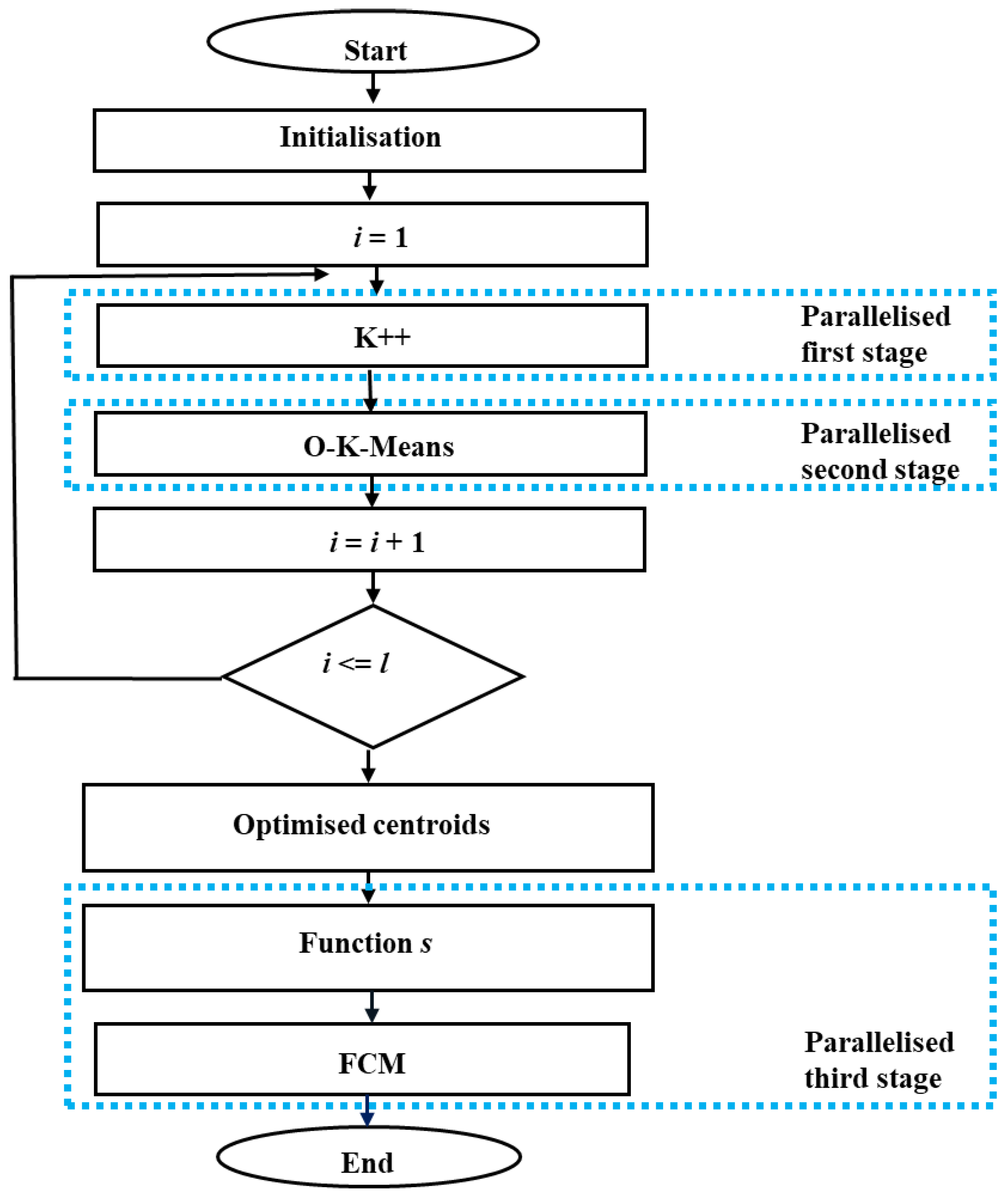
4.2. Proposed POFCM Algorithm

To explain our proposal, we rely on Figure 1, which shows the hybrid and parallel approach, and on Algorithm 5, where the parallel implementation is detailed.

Figure 1 shows the parallel and hybrid approach of the POFCM algorithm. It can be seen that the parallel implementation is divided into three stages, which are indicated by dashed lines. The first stage is the parallelisation of the K++ algorithm. The second stage is the parallelisation of the O-K-Means algorithm. Note that our algorithm repeats the execution of K++ and O-K-Means l times and selects the run with the lowest objective function value from the l solutions. In this research, we select the value of 10 based on a set of experiments with different values of l. We observe that the value of l = 10 provides good results in general. The above is the basis for selecting the set of final centroids. These final centroids are transformed into a membership matrix using the function s. The membership matrix is provided as input parameters to the FCM algorithm. The s function and the standard FCM are parallelised in the third stage.

Algorithm 5 shows the four implementation phases of our POFCM algorithm. The input parameters are the dataset X, the number of clusters c, the weighting exponent m, the threshold value ε (stopping criteria for the FCM algorithm), the threshold value εok (stopping criteria for the O-K-Means algorithm), the number of threads T, the iteration counter r, the iteration counter i, and the stop variable. The output parameters are the set of centroids V and the values of the membership matrix U. The first is the initialisation phase. The block of instructions that corresponds to this phase consists of lines 1 to 13. The variable i is initialised to 1. Inside the repeat-while loop, there are two functions: (a) Line 4 shows the parallelised K++ function, which has the input parameters X, c, and T; this function returns the set of centroids V′. (b) Line 6 invokes the parallelised O-K-Means function, which has the input parameters X, V′, εok, c, and T; this function returns the set of centroids V″. In line 10, the solution with the lowest value of the objective function and its final centroids V″ is determined. Line 11 shows the parallelised s function, which maps the final centroids V″ to the values of the membership matrix U. In line 13, the iteration counter r of the FCM algorithm is initialised.

The second phase of the POFCM algorithm, called calculate centroids, consists of lines 14 to 17. Line 15 invokes the parallelised centroid function, which has the input parameters X, U, m, and T; this function returns the set of centroids V′. The calculation of centroids is performed using Equation (2), described in Section 2. This phase returns the new set of centroids V.

The third phase, called classification, is shown between lines 18 and 21. Line 19 shows the parallelised classification function, which has the input parameters X, V, m, and T; this function returns the set of centroids V′. The values of the membership matrix are calculated and updated using Equation (3). This phase returns the values of the membership matrix U.

Finally, the convergence phase is shown from lines 22 to 32. Line 23 invokes the parallelised convergence function, which has the input parameters X, U, m, ε, T, r, and stop. This phase allows for obtaining the maximum absolute value of the values of the membership matrix in two consecutive iterations, as seen in line 24. If these obtained values are less than the threshold ε, the value of 0 is assigned to the stop variable, the values of the membership matrix U and stop value are returned, and the algorithm stops. Otherwise, the values of the membership matrix U are updated, the iteration counter r is increased, the value of 1 is assigned to the stop variable, and the values of the membership matrix U and stop are returned, as can be seen in line 30. In line 31, if the stop variable equals 1, the algorithm returns to the centroid calculation phase.

Algorithm 5: POFCM
Input: dataset X, c, m, ε, εok, T, r, i, stop;
Output: V, U;
1	Initialisation:
2	i: = 1;
3	Repeat
4	Function K++ (X, c, T): //This function was parallelised.
5	Return V’;
6	Function O-K-Means (X, V’, εok, c, T): //This function was parallelised.
7	Return V’’;
8	i = i + 1;
9	While i <= l;
10	Select V’’ for the value of i at which the objective function obtained the minimum value;
11	Function s (X, V’’, m, T); //This function was parallelised.
12	Return U;
13	r: = 1;
14	Calculate centroids:
15	Function Centroids (X, U, m, T); //This function was parallelised.
16	//Calculate the centroids using Equation (2);
17	Return V;
18	Classification:
19	Function Classification (X, V, m, T); //This function was parallelised.
20	//Update and calculate the membership matrix using Equation (3);
21	Return U;
22	Convergence:
23	Function Convergence (X, U, ε, T, r, stop); //This function was parallelised.
24	If max [abs(µij(r) − µij(r+1))] < ε then:
25	stop: = 0;//The stop flag of the algorithm is activated.
26	Return U, stop;
27	Otherwise:
28	U(r): = U(r+1) and r: = r + 1;
29	stop: = 1;
30	Return U, stop;
31	If stop = 1 then go to Calculate centroids
32	End of algorithm

In general, the parallelisation coding includes the pragma directive just before the first for loop of the K++, O-K-Means, s, centroids, classification, and convergence functions. In addition, some of these functions contain nested subfunctions; in these subfunctions, the pragma directive is included just before the first for loop. However, some cases require specific clauses to ensure proper processing in the parallel environment. An example of these clauses is private (i), which guarantees that the values of the variables declared between the parentheses can only be shared in the loop associated with the pragma directive.

5. Evaluation

This section presents the experimental setup, the description of the datasets, the test cases, and the metrics used to evaluate the quality of the POFCM algorithm.

5.1. Experimental Setup

To evaluate the solutions of the proposed improvement, the HOFCM and POFCM algorithms were implemented. These algorithms were implemented in C language with the Microsoft Visual C++ (MSVC) 2020 compiler and OpenMP version 2.0. The computer equipment used had the following characteristics: Intel^® Core^TM i5-4570 at 3.30 GHz, 4 processors, 14 GB RAM, and 512 GB HDD storage with a Windows 10 operating system.

5.2. Description of the Datasets

The real datasets were obtained from the UCI machine learning repository [46]. A set of 16 synthetic datasets was created, and the values of their attributes were randomly generated with a uniform distribution and an interval from 1 to 10.

Table 2. Datasets used in experiments.

ID	Name	Type	n	d	Size Indicator n × d
1	ABALONE	Real	4177	7	29,239
2	SPAM	Real	4601	57	262,257
3	URBAN	Real	360,177	2	720,354
4	S10_10	Synthetic	10,000	10	100,000
5	S10_20	Synthetic	10,000	20	200,000
6	S10_30	Synthetic	10,000	30	300,000
7	S10_40	Synthetic	10,000	40	400,000
8	S20_10	Synthetic	20,000	10	200,000
9	S20_20	Synthetic	20,000	20	400,000
10	S20_30	Synthetic	20,000	30	600,000
11	S20_40	Synthetic	20,000	40	800,000
12	S30_10	Synthetic	30,000	10	300,000
13	S30_20	Synthetic	30,000	20	600,000
14	S30_30	Synthetic	30,000	30	900,000
15	S30_40	Synthetic	30,000	40	1,200,000
16	S40_10	Synthetic	40,000	10	400,000
17	S40_20	Synthetic	40,000	20	800,000
18	S40_30	Synthetic	40,000	30	1,200,000
19	S40_40	Synthetic	40,000	40	1,600,000

provides details of the datasets used. The table structure is as follows: column one shows the dataset identifier, column two contains the name; column three indicates the data type; columns four and five contain the number of objects and dimensions of the dataset; column six shows the product of columns four and five.

5.3. Test Cases

The test cases were designed to contrast the results of our proposal with respect to the HOFCM algorithm. In particular, the metrics to evaluate performance were speedup and parallel efficiency, as shown in Equations (9) and (10). Two experiments were designed. The purpose of Experiment I was to solve the real datasets, and the purpose of Experiment II was to solve the synthetic datasets.

5.3.1. Description of Experiment I

The purpose of this experiment was to contrast the results of the HOFCM and POFCM algorithms for the three real datasets: ABALONE, SPAM, and URBAN. The configuration of the input parameters for the execution of the two algorithms was m = 2 and ε = 0.01 (these values were proposed as reasonable values in [39]), εok = 0.72 (the εok value of the O-K-Means algorithm was the proposed value as a result of the investigation in [41]), and c = 2, 4, 6, 8, 10, 14, 18, and 26. It is important to note that the input parameters were the same as those used in the HOFCM algorithm [20].

Each dataset was solved 10 times with both algorithms. This value was selected based on preliminary tests in which a sample size of 10 runs was found to provide good results.

5.3.2. Description of Experiment II

The purpose of this experiment was to contrast the results of HOFCM and POFCM when solving the 16 synthetic datasets. The datasets were divided into four subgroups: the first from S10_10 to S10_40, with 10,000 objects; the second from S20_10 to S20_40, with 20,000 objects; the third from S30_10 to S30_40, with 30,000 objects; finally, the fourth subgroup from S40_10 to S40_40, with 40,000 objects. In turn, each subgroup was divided into four instances, where the numbers of dimensions were d = 10, 20, 30, and 40. The configuration of the input parameters for the execution of the two algorithms was: m = 2; ε = 0.01; εok = 0.72; c = 2, 12, 22, and 32.

As in Experiment I, each dataset was solved 10 times with both algorithms.

5.4. Metrics

The speedup (Sp) and parallel efficiency (Pe) are two metrics used to evaluate the quality of a parallel algorithm. The rate of acceleration or speedup indicates the relationship between the sequential execution time (Ts), in this case, the time of the HOFCM algorithm and the parallel execution time (Tp), as shown in Equation (9). The ideal speedup is a linear value Sp = p, where p is the number of processors [47]. The parallel efficiency indicates the relationship between the speedup and the number of processors used p, as shown in Equation (10). The ideal parallel efficiency value is 1 [47].

$$Sp=\frac{Ts}{Tp}$$

(9)

$$Pe=\frac{Sp}{p}$$

(10)

As an example, the sequential and parallel execution time is shown in seconds for the URBAN and S40_40 datasets.

$$\begin{array}{cc}\begin{array}{c}\mathit{Ts}=1143.2\mathrm{s}\hfill \\ \mathit{Tp}=304.09\mathrm{s}\hfill \end{array}\hfill & \hfill S{p}_{URBAN}=\frac{1143.2}{304.09}=3.76\hspace{1em}P{e}_{URBAN}=\frac{3.76}{4}=0.94\\ p=4\mathrm{processors}\hfill & \\ c=32\hfill & \end{array}$$

$$\begin{array}{cc}\begin{array}{c}\mathrm{Ts}=1584.6\mathrm{s}\hfill \\ \mathit{Tp}=400.4\mathrm{s}\hfill \end{array}\hfill & \hfill S{p}_{s\mathit{40}\_\mathit{40}}=\frac{1584.6}{400.4}=3.96\hspace{1em}P{e}_{s\mathit{40}\_\mathit{40}}=\frac{3.96}{4}=0.99\\ p=4\mathrm{processors}\hfill & \\ c=32\hfill & \end{array}$$

6. Results

This section shows the results of the dataset solution using the HOFCM and POHCM algorithms for Experiments I and II.

Table 3. Results of Experiment I.

	ABALONE		SPAM		URBAN
Cluster	Speedup Sp	Parallel Efficiency Pe	Speedup Sp	Parallel Efficiency Pe	Speedup Sp	Parallel Efficiency Pe
2	1.88	0.47	1.78	0.45	1.87	0.47
4	2.10	0.53	2.31	0.58	2.48	0.62
6	2.61	0.65	2.58	0.64	2.79	0.70
8	2.82	0.70	3.24	0.81	3.35	0.84
10	3.13	0.78	3.14	0.79	3.12	0.78
14	3.39	0.85	3.50	0.88	3.45	0.86
18	3.49	0.87	3.60	0.90	3.55	0.89
26	3.60	0.90	3.64	0.91	3.76	0.94

shows the average results of 10 executions obtained in terms of speedup and parallel efficiency.

As can be seen in Table 3, as the number of clusters increased, the speedup and parallel efficiency tended to their upper limit values. Note that for the ABALONE dataset, the speedup exceeded the value of 3 from c = 10 onwards. In contrast, for the other datasets, which were larger, the speedup exceeded the value of 3 from c = 8 onwards.

Figure 2 shows the speedup of the three real datasets ABALONE, SPAM, and URBAN. The number of clusters is on the x-axis, and the speedup is on the y-axis. Note that the best speedup result was 3.76 and was obtained by solving the URBAN dataset for 26 clusters.

Figure 3 shows the speedup values for the 16 synthetic datasets. The x-axis represents the number of clusters and the number of dimensions of each dataset. The y-axis represents speedup. On the far right of the figure is a colour code indicating the number of objects in each dataset.

6.1. Analysis of Results

This section analyses the results obtained after solving the problems described in Experiments I and II.

6.1.1. Analysis of the Results of Experiment I

Based on the experimental results shown in Table 3 and Figure 2, where the results of the sequential HOFCM and POFCM algorithms are shown, the following was observed:

• For the three datasets, speedup and parallel efficiency tended to improve as the number of clusters increased.
• It was found relevant that for a value of c greater than or equal to 10, the values of speedup and parallel efficiency tended to their upper-limit values.
• In the best case, POFCM reduced the execution time by 73.4% of the time required by the HOFCM algorithm to solve the URBAN dataset with 26 clusters.
• It is worth noting that the quality with POFCM was the same as with HOFCM.

6.1.2. Analysis of the Results of Experiment II

Considering the results shown in Figure 3, the following was observed:

• When solving the 16 synthetic datasets, it was found that with POFCM, in addition to increasing the speedup when the number of clusters increases, the speedup also increased when the dimension of the datasets grew.
• When running the synthetic dataset S10_10, considered the smallest, the speedup achieved a value of 3.5 for 32 clusters.
• In the best cases, the solution time was reduced by up to 74.7% for the S40_40 dataset of 10,000 objects and 40 dimensions. With this same dataset, a speedup of 3.96 was achieved. It is important to note that this speedup value is higher than other reported values.

6.1.3. Comparative Analysis with Other Works

As shown in column four of Table 1, there are few works on fuzzy clustering parallel algorithms with OpenMP. In particular, we only identified one article with which we could compare our results [37]. Therefore, to compare results, we selected the experiment with the best results from reference [37] and our own study. The experiments solved the datasets ten times, and the average times are shown.

Data from experiments in article [37]:

The dataset was 241,200 pixels in size and the number of clusters was 16. The results were the following: an average of 107.315 s in 10 runs for the sequential version, an average of 55.092 s in 10 runs for the parallel version, a speedup of 1.95, and a parallel efficiency of 0.97.

Data from our experiments with the synthetic dataset S40_40:

The dataset was 40,000 objects in size and 40 dimensions; the number of clusters was 32. The results were the following: an average time of 1584.6 s in 10 runs for the sequential version, an average of 400.4 s in 10 runs for the parallel version, a speedup of 3.96, and a parallel efficiency of 0.99.

It can be seen that the implementation has a higher parallel efficiency than that of reference [37]. Furthermore, it is noteworthy that in the referenced article, the tests were carried out using only one dataset; in contrast, in our research, the experimentation was carried out with 19 datasets, which allowed us to characterise our algorithm better.

7. Conclusions

This article shows that it is feasible to parallelise in OpenMP the HOFCM algorithm, which is a variant of the FCM algorithm. To validate our proposal, which we call POFCM, a set of experiments was designed with three real datasets from the UCI repository [46] and 16 synthetic datasets. Our approach showed a significant reduction in solution time while maintaining the quality of the solution. All the datasets were solved with the HOFCM and POFCM algorithms, with different values for the number of cluster parameters. Based on the results, it was observed that POFCM had a better solution time than HOFCM. In the best case, it reduced the solution time by up to 73.4% when solving the URBAN dataset and 74.7% with a synthetic dataset with 40,000 objects and 40 dimensions. Our approach achieved speedup values of up to 3.96 and a parallel efficiency value of 0.99. Regarding parallel efficiency, our approach surpassed results from other publications. It is noteworthy that POFCM tended to improve processing times as the number of dimensions and clusters increased. This feature is particularly useful in solving massive datasets. Our main contribution is a fuzzy clustering algorithm for large datasets that is scalable and not limited to a specific domain. Finally, it is suggested that future work consists in implementing POFCM in parallel with distributed memory, allowing the use of more resources and thus increasing its speed.

References

1. Statista Research Departmen. Volume of Data/Information Created, Captured, Copied, and Consumed Worldwide from 2010 to 2020, with Forecasts from 2021 to 2025. Available online: https://www.statista.com/statistics/871513/worldwide-data-created/ (accessed on 13 November 2022).
2. Shirkhorshidi, A.S.; Aghabozorgi, S.; Wah, T.Y.; Herawan, T. Big Data Clustering: A Review. In Proceedings of the Computa-tional Science and Its Applications—ICCSA 2014, Guimaraes, Portugal, 30 June–3 July 2014. [Google Scholar]
3. Ajin, V.W.; Kumar, L.D. Big data and clustering algorithms. In Proceedings of the 2016 International Conference on Research Advances in Integrated Navigation Systems (RAINS), Bangalore, India, 6–7 April 2016. [Google Scholar]
4. Bezdek, J. Elementary Cluster Analysis: Four Basic Methods that (Usually) Work; River Publishers: New York, NY, USA, 2022; pp. 1–10. [Google Scholar]
5. Nayak, J.; Naik, B.; Behera, H.S. Fuzzy C-Means (FCM) Clustering Algorithm: A Decade Review from 2000 to 2014. In Proceedings of the Computational Intelligence in Data Mining, Odisha, India, 20–21 December 2014. [Google Scholar]
6. Mahdi, M.A.; Hosny, K.M.; Elhenawy, I. Scalable Clustering Algorithms for Big Data: A Review. IEEE Access 2021, 9, 80015–80027. [Google Scholar] [CrossRef]
7. Bonilla, J.; Vélez, D.; Montero, J.; Rodríguez, J.T. Fuzzy Clustering Methods with Rényi Relative Entropy and Cluster Size. Mathematics 2021, 9, 1423. [Google Scholar] [CrossRef]
8. MacQueen, J. Some methods for classification and analysis of multivariate observations. In Proceedings of the 5th Berkeley Symposium on Mathematical Statistics and Probability, Berkeley, CA, USA, 21 June–18 July 1965. [Google Scholar]
9. Lee, G.M.; Gao, X. A Hybrid Approach Combining Fuzzy c-Means-Based Genetic Algorithm and Machine Learning for Predicting Job Cycle Times for Semiconductor Manufacturing. Appl. Sci. 2021, 11, 7428. [Google Scholar] [CrossRef]
10. Lee, S.J.; Song, D.H.; Kim, K.B.; Park, H.J. Efficient Fuzzy Image Stretching for Automatic Ganglion Cyst Extraction Using Fuzzy C-Means Quantization. Appl. Sci. 2021, 11, 12094. [Google Scholar] [CrossRef]
11. Dunn, J.C. A Fuzzy Relative of the ISODATA Process and Its Use in Detecting Compact Well-Separated Clusters. J. Cybern. 1974, 3, 32–57. [Google Scholar] [CrossRef]
12. Bezdek, J.C. Pattern Recognition with Fuzzy Objective Function Algorithms; Plenum Press: New York, NY, USA, 1981; pp. 43–93. [Google Scholar]
13. Ghosh, S.; Kumar, S. Comparative Analysis of K-Means and Fuzzy C-Means Algorithms. Int. J. Adv. Comput. Sci. Appl. 2013, 4, 35–39. [Google Scholar] [CrossRef]
14. Garey, M.R.; Johnson, D.S. Computers and Intractability: A Guide to the Theory of NP-Completeness; W. H. Freeman & Co.: New York, NY, USA, 1979; pp. 109–120. [Google Scholar]
15. Barrah, H.; Cherkaoui, A. Fast Robust Fuzzy Clustering Algorithm for Grayscale Image Segmentation. In Proceedings of the Xth International Conference on Integrated Design and Production, Tangier, Morocco, 2–4 December 2015. [Google Scholar]
16. Hashemzadeh, M.; Golzari Oskouei, A.; Farajzadeh, N. New fuzzy C-means clustering method based on feature-weight and cluster-weight learning. Appl. Soft Comput. 2019, 78, 324–345. [Google Scholar] [CrossRef]
17. Stetco, A.; Zeng, X.J.; Keane, J. Fuzzy C-means++: Fuzzy C-means with effective seeding initialization. Expert Syst. Appl. 2015, 42, 7541–7548. [Google Scholar] [CrossRef]
18. Wu, Z.; Chen, G.; Yao, J. The Stock Classification Based on Entropy Weight Method and Improved Fuzzy C-means Algorithm. In Proceedings of the 4th International Conference on Big Data and Computing, Guangzhou, China, 10–12 May 2019. [Google Scholar]
19. Liu, Q.; Liu, J.; Li, M.; Zhou, Y. Approximation algorithms for fuzzy C-means problem based on seeding method. Theor. Comput. Sci. 2021, 885, 146–158. [Google Scholar] [CrossRef]
20. Pérez, J.; Roblero, S.S.; Almanza, N.N.; Solís, J.F.; Zavala, C.; Hernández, Y.; Landero, V. Hybrid Fuzzy C-Means Clustering Algorithm Oriented to Big Data Realms. Axioms 2022, 11, 377. [Google Scholar] [CrossRef]
21. Manacero, A.; Guariglia, E.; de Souza, T.A.; Lobato, R.S.; Spolon, R. Parallel fuzzy minimals on GPU. Appl. Sci. 2022, 12, 2385. [Google Scholar] [CrossRef]
22. Zhang, Q.; Chen, Z.; Leng, Y. Distributed fuzzy c-means algorithms for big sensor data based on cloud computing. Int. J. Sens. Netw. 2015, 18, 32. [Google Scholar] [CrossRef]
23. Qin, J.; Fu, W.; Gao, H.; Zheng, W.X. Distributed k-Means Algorithm and Fuzzy c-Means Algorithm for Sensor Networks Based on Multiagent Consensus Theory. IEEE Trans. Cybern. 2016, 47, 772–783. [Google Scholar] [CrossRef] [PubMed]
24. Al-Ayyoub, M.; Abu-Dalo, A.M.; Jararweh, Y.; Jarrah, M.; Sa’d, M.A. A GPU-based implementations of the fuzzy C-means algorithms for medical image segmentation. J. Supercomput. 2015, 71, 3149–3162. [Google Scholar] [CrossRef]
25. Ali, N.A.; Cherradi, B.; Abbassi, A.E.; Bouattane, O.; Youssfi, M. New parallel hybrid implementation of bias correction fuzzy C-means algorithm. In Proceedings of the 2017 International Conference on Advanced Technologies for Signal and Image Processing (ATSIP), Fez, Morocco, 22–24 May 2017. [Google Scholar]
26. Al-Ayyoub, M.; Al-andoli, M.; Jararweh, Y.; Smadi, M.; Gupta, B. Improving fuzzy C-mean-based community detection in social networks using dynamic parallelism. Comput. Electr. Eng. 2018, 74, 533–546. [Google Scholar] [CrossRef]
27. AlZu’bi, S.; Shehab, M.; Al-Ayyoub, M.; Jararweh, Y.; Gupta, B. Parallel implementation for 3D medical volume fuzzy segmentation. Pattern Recognit. Lett. 2020, 130, 312–318. [Google Scholar] [CrossRef]
28. Cecilia, J.M.; Cano, J.-C.; Morales-García, J.; Llanes, A.; Imbernón, B. Evaluation of Clustering Algorithms on GPU-Based Edge Computing Platforms. Sensors 2020, 20, 6335. [Google Scholar] [CrossRef]
29. Cebrian, J.M.; Imbernón, B.; Soto, J.; Cecilia, J.M. Evaluation of Clustering Algorithms on HPC Platforms. Mathematics 2021, 9, 2156. [Google Scholar] [CrossRef]
30. Ali, N.A.; Abbassi, A.E.; Cherradi, B. The performances of iterative type-2 fuzzy C-mean on GPU for image segmentation. J. Supercomput. 2022, 78, 1583–1601. [Google Scholar] [CrossRef]
31. Liu, B.; He, S.; He, D.; Zhang, Y.; Guizani, M. A Spark-based Parallel Fuzzy C-means Segmentation Algorithm for Agricultural Image Big Data. IEEE Access 2019, 7, 42169–42180. [Google Scholar] [CrossRef]
32. Ma, Y.; Cheng, W. Optimization and Parallelization of Fuzzy Clustering Algorithm Based on the Improved Kmeans++ Clustering. IOP Conf. Ser. Mater. Sci. Eng. 2020, 768, 072106. [Google Scholar] [CrossRef]
33. Yu, Q.; Ding, Z. An improved Fuzzy C-Means algorithm based on MapReduce. In Proceedings of the 2015 8th International Conference on Biomedical Engineering and Informatics (BMEI), Shenyang, China, 14–16 October 2015. [Google Scholar]
34. Dai, W.; Yu, C.; Jiang, Z. An Improved Hybrid Canopy-Fuzzy C-Means Clustering Algorithm Based on MapReduce Model. J. Comput. Sci. Eng. 2016, 10, 1–8. [Google Scholar] [CrossRef]
35. Sardar, T.H.; Ansari, Z. MapReduce-based Fuzzy C-means Algorithm for Distributed Document Clustering. J. Inst. Eng. India Ser. B 2022, 103, 131–142. [Google Scholar] [CrossRef]
36. Almomany, A.; Jarrah, A.; Al Assaf, A.H. FCM Clustering Approach Optimization Using Parallel High-Speed Intel FPGA Technology. J. Electr. Comput. Eng. 2022, 2022, 8260283. [Google Scholar] [CrossRef]
37. Sakarya, O. Applying fuzzy clustering method to color image segmentation. In Proceedings of the 2015 Federated Conference on Computer Science and Information Systems, Lodz, Poland, 13–16 September 2015. [Google Scholar]
38. Vela-Rincón, V.V.; Mújica-Vargas, D.; de Jesus Rubio, J. Parallel hesitant fuzzy C-means algorithm to image segmentation. Signal Image Video Process. 2022, 16, 73–81. [Google Scholar] [CrossRef]
39. Bezdek, J.C.; Ehrlich, R.; Full, W. FCM: The fuzzy c-means clustering algorithm. Comput. Geosci. 1984, 10, 191–203. [Google Scholar] [CrossRef]
40. Arthur, D.; Vassilvitskii, S. k-means++: The Advantages of Careful Seeding. In Proceedings of the Eighteenth Annual ACM-SIAM Symposium on Discrete Algorithms, New Orleans, LA, USA, 7–9 January 2007. [Google Scholar]
41. Pérez, J.; Almanza, N.N.; Romero, D. Balancing effort and benefit of K-means clustering algorithms in Big Data realms. PLoS ONE 2018, 13, e0201874. [Google Scholar] [CrossRef]
42. Ruspini, E.H. A new approach to clustering. Inf. Control 1969, 15, 22–32. [Google Scholar] [CrossRef]
43. Chandra, R.; Dagum, L.; Kohr, D.; Menon, R.; Maydan, D.; McDonald, J. Parallel Programming in OpenMP; Academic Press: San Diego, CA, USA, 2001; pp. 2–9. [Google Scholar]
44. Schmidt, B.; Gonzalez-Dominguez, J.; Hundt, C.; Schlarb, M. Parallel Programming: Concepts and Practice; Elsevier Science: Cambridge, MA, USA, 2017; pp. 165–179. [Google Scholar]
45. OpenMP. Application Programming Interface. Available online: https://www.openmp.org/wp-content/uploads/openmp-examples-4.5.0.pdf (accessed on 20 January 2023).
46. UCI Machine Learning Repository, University of California. Available online: https://archive.ics.uci.edu/ml/index.php (accessed on 26 November 2022).
47. Zavala-Díaz, J.C.; Cruz-Chávez, M.A.; López-Calderón, J.; Hernández-Aguilar, J.A.; Luna-Ortíz, M.E. A Multi-Branch-and-Bound Binary Parallel Algorithm to Solve the Knapsack Problem 0–1 in a Multicore Cluster. Appl. Sci. 2019, 9, 5368. [Google Scholar] [CrossRef]
Figure 1. Parallelised implementation of POFCM algorithm.
Mathematics 11 01920 g001
Figure 2. Speedup of Experiment I.
Mathematics 11 01920 g002
Figure 3. Speedup of Experiment II.
Mathematics 11 01920 g003