Abstract
A limited feasible region restricts individuals from evolving optionally and makes it more difficult to solve constrained optimization problems. In order to overcome difficulties such as introducing initial feasible solutions, a novel algorithm called the successive approximation genetic algorithm (SAGA) is proposed; (a) the simple genetic algorithm (SGA) is the main frame; (b) a self-adaptive penalty function is considered and the penalty factor is adjusted automatically by the proportion of feasible and infeasible solutions; (c) a generation-by-generation approach and a three-stages evolution are introduced; and (d) dynamically enlarging and reducing the tolerance error of the constraint violation makes it much easier to generate initial feasible solutions. Then, ten benchmarks and an engineering problem were adopted to evaluate the SAGA in detail. It was compared with the improved dual-population genetic algorithm (IDPGA) and eight other algorithms, and the results show that SAGA finds the optimum in 5 s for an equality constraint and 1 s for an inequality constraint. The largest constraint violation can be accurate to at least three decimal fractions for most problems. SAGA obtains a better value, of 1.3398, than the eight other algorithms for the engineering problem. In conclusion, SAGA is very suitable for solving nonlinear optimization problems with a single constraint, accompanied by more accurate solutions, but it takes a longer time. In reality, SAGA searched for a better solution along the bound after several iterations and converged to an acceptable solution in early evolution. It is critical to improve the running speed of SAGA in the future.
Keywords:
successive approximation; genetic algorithm; nonlinear constrained optimization; single constraint; self-adaptive; SAGA MSC:
90C59; 90-08
1. Introduction
As novel and efficient optimization algorithms, heuristic algorithms have been applied widely in many kinds of optimization areas, such as the sizing, topology and geometry optimization of steel structures [1], the optimization of the seismic behavior of steel planar frames with semi-rigid connections [2] and so on [3,4,5,6,7,8]. Heuristic algorithms have remarkable advantages over mathematical programming methods; for example, the relevant derivative information of objectives, including the first-order Jacobian matrix or second-order Hessian matrix, is not needed to solve problems, and continuous or convex design regions or explicit constraints are not required. The genetic algorithm (GA) described by Holland [9] is a typical and the most-used heuristic algorithm and is composed of population initialization and calculating fitness, judgments, iterations, evaluations and updates. Moreover, other intelligent algorithms also have been proposed and utilized to solve various optimization problems, such as the simulated annealing algorithm [10], particle swarm algorithm [11], neural networks [12], ant colony algorithm [13], artificial fish swarm algorithm [14], firefly algorithm [15], cuckoo search [16], etc.
Genetic algorithms search for the optimum by imitating natural phenomena or referring to life experience, which has been demonstrated to be very efficient and low-cost in practice. In the past, many studies have studied and improved genetic algorithms to solve unconstrained and constrained optimization problems and achieved the desired effect. Nonlinear constrained optimization problems are more difficult to deal with than unconstrained optimization problems in practice, because the limited feasible region restricts individuals from evolving optionally, and inappropriate constraint handling can easily cause the algorithm to converge to an infeasible solution or a feasible solution far from the optimum, or even fail to converge. A general form of nonlinear constrained optimization problems is shown in Equation (1), where and are inequality constraints and equality constraints, respectively, and at least one of objectives and constraints is nonlinear.
The most common way to deal with constraints is to convert the constraints to objectives by introducing penalty functions in constrained optimization problems. The objective function is represented as shown in Equation (2); is the objective after conversion, is a penalty factor, is a combined penalty item and is a small positive number that represents the tolerance error of an equality constraint.
Thus, the original constrained problem is converted to an unconstrained problem, as shown in Equation (3).
Many studies on constraint handling have been conducted in the literature. Typical penalty functions include static penalty functions [17,18,19], dynamic penalty functions [20,21], annealing penalty functions [20,22,23], self-adaptive penalty functions [24,25,26], etc. The details will be explained below. Furthermore, there are some other studies on constraint handling. Deb [27] exploited GA’s population-based approach and ability to make pair-wise comparisons in a tournament selection operator to devise a penalty function approach, in which any penalty parameter is not required; then, feasible and infeasible solutions are compared carefully, once sufficient feasible solutions are found,. A niching method (along with a controlled mutation operator) is used to maintain diversity among feasible solutions. Shang et al. [28] proposed a hybrid flexible tolerance genetic algorithm (FTGA) to solve nonlinear, multimodal and multi-constraint optimization problems, in which, as one of the adaptive genetic algorithm (AGA) operators, a flexible tolerance method (FTM) is organically merged into an AGA. Li and Du [29] proposed a boundary simulation method to address inequality constraints for GAs, which can efficiently generate a feasible region boundary point set to approximately simulate the boundary of the feasible region. Meanwhile, they proposed a series of genetic operators that abandon or repair infeasible individuals produced during the search process. Montemurro et al. [30] proposed the Automatic Dynamic Penalization (ADP) method, which belongs to the category of exterior penalty-based strategies, in which in order to guide the search through the whole definition domain and to achieve a proper evaluation of the penalty coefficients, it is possible to exploit the information restrained in the population at the current generation. Liang et al. [31] proposed a genetic algorithm to handle constraints which searches the decision space of a problem through the arithmetic crossover of feasible and infeasible solutions, and performs a selection on feasible and infeasible populations, respectively, according to fitness and constraint violations. Meanwhile, the algorithm uses the boundary mutation on feasible solutions and the non-uniform mutation on infeasible solutions and maintains the population diversity through dimension mutation. Garcia et al. [32] presented a constraint handling technique (CHT) called the Multiple Constraint Ranking (MCR), which extends the rank-based approach from many CHTs by building multiple separate queues based on the values of the objective function and the violation of each constraint and overcomes difficulties found by other techniques when faced with complex problems characterized by several constraints with different orders of magnitude and/or different units. Miettinen et al. [33] studied five penalty function-based constraint handling techniques to be used with genetic algorithms in global optimization and discovered the method of adaptive penalties turns out to be most efficient, while the method of parameter-free penalties is the most reliable. Yuan et al. [34] combined the genetic algorithm with hill-climbing search steps to propose a new algorithm which can be widely applied to a class of global optimization problems for continuous functions with box constraints. A repair procedure was proposed by Chootinan and Chen [35] and embedded into a simple GA as a special operator, in which the gradient information derived from the constraint set is used to systematically repair infeasible solutions. Without defining membership functions for fuzzy numbers, Lin [36] used the extension principle, interval arithmetic and alpha-cut operations for fuzzy computations, and a penalty method for constraint violations to investigate the possibility of applying GAs to solve this kind of fuzzy linear programming problem. Hassanzadeh et al. [37] considered nonlinear optimization problems constrained by a system of fuzzy relation equations and proposed a genetic algorithm with max-product composition to obtain a near-optimal solution for convex or nonconvex solution sets. Abdul-Rahman et al. [38] proposed a Binary Real-coded Genetic Algorithm (BRGA) which combines cooperative Binary-coded GA (BGA) with Real-coded GA (RGA), then introduced a modified dynamic penalty function into the architecture of the BRGA and extended the BRGA to constrained problems. Tsai and Fu [39] presented two genetic-algorithm-based algorithms that adopt different sampling rules and searching mechanisms to consider the discrete optimization via simulation problem with a single stochastic constraint. Zhan [40] proposed a genetic algorithm based on annealing infeasible degree selection for constrained optimization problems which shows great simulation results.
In order to explore the potential of genetic algorithms adequately and develop an algorithm suitable for engineering optimization, this paper proposes a novel and efficient genetic algorithm named the successive approximation genetic algorithm (SAGA) for nonlinear constrained optimization problems with a single constraint, considering a self-adaptive penalty function, dividing solution space into feasible and infeasible solutions and introducing a generation-by-generation approaching strategy. The performance of SAGA was evaluated in detail through a series of mathematical and engineering optimization problems; then, comparing it with other existing algorithms, it was further proved that SAGA has better accuracy and robustness. Considering that existing algorithm scripts are mostly written in MATLAB while the open source language Python is growing in popularity, all scripts in this paper were completed in Python and its third-party library, including the main program of SAGA (Python and Numpy), the images of the objectives and contour lines or surfaces (Numpy, Matplotlib and Mayavi), writing the results into the text (Python and Pandas), etc.
2. Related Work on Typical Penalty Functions
Just a few typical penalty functions are listed here. The equation constraint is usually converted as , where is a small positive number. This section briefly summarizes some commonly used penalty function methods.
2.1. Static Penalty Functions
The penalty function proposed by Homaifar, Qi and Lai [17] is shown in Equation (4). The constraint violation is divided into several levels; is a penalty factor and is the number of constraint violations after converting the equation constraints to inequation constraints.
Like a unilateral penalty, Hoffmeister and Sprave [18] proposed the penalty function shown in Equation (5) and adopted the Heavyside function .
Kuri and Quezada [19] proposed the penalty function shown in Equation (6), where is the number of constraints, is the number of constraints met and is a very large number; they suggested .
2.2. Dynamic Penalty Functions
Joines and Houck [20] proposed the dynamic penalty function shown in Equation (7), where , and are three constants—they suggested 0.5, 1 or 2 and 1 or 2, respectively— is the current generation and and are the inequality and equality penalty item, respectively.
2.3. Annealing Penalty Functions
Joines and Houck [20] proposed another annealing penalty function, shown in Equation (8), where the meanings of parameters are the same as above, and , and are suggested to be 0.05, 1 and 1, respectively.
Michalewicz and Attia [22] divided constraints into four categories: linear equality constraints, nonlinear equality constraints, linear inequality constraints and nonlinear inequality constraints; then, they proposed the annealing penalty function shown in Equation (9), where is a variable parameter and gradually decreases based on iterations.
Carlson and Shonkwiler [23] proposed a similar annealing penalty function, shown in Equation (10), where is a distance parameter and is a time parameter that gradually decreases to zero.
2.4. Self-Adaptive Penalty Functions
Hadj-Alouane and Bean [26] utilized the feedback of search process to propose a new self-adaptive penalty function, shown in Equation (11), where , case1 means all best solutions belong to feasible region in the previous k iterations, and case2 means all best solutions belong to infeasible region in the previous k iterations.
3. Methodology
The penalty functions listed above have achieved delightful results in actual application, but have also faced some difficulties, for instance, the accurate parameters are difficult to select, an initial feasible solution that satisfies many constraints needs to be introduced beforehand and so on. The proposed successive approximation genetic algorithm (SAGA) in this paper adopts a series of easy and efficient strategies and gradually searches for the global optimum based on iterations. The main frame of SAGA is still a simple genetic algorithm (SGA). This section explains each part of SAGA in detail.
3.1. The Penalty Function of SAGA
The penalty function form in Equation (2) is still adopted for constraint handling in SAGA, and a self-adaptive penalty function is utilized in which it is critical to select the penalty factor . should be a larger value in the earlier evolution because there are fewer feasible solutions, and should gradually decrease as iterations go on. The penalty factor selected in the paper is referred to by Cai [41], as shown in Equation (12), where represents the proportion of feasible solutions, and represent the number of feasible solutions and all solutions, respectively, and is used to control the range of penalty factors, and a large positive integer is generally preferred.
The penalty factor changes with ; when equals zero, no feasible solutions exist and reaches the maximum; when equals one, all solutions are feasible and reaches the minimum and equals zero, which means no individual needs to be penalized. One great advantage of such a penalty function is that the penalty factor is not too large or small, changes dynamically with the population and does not need to be specified manually.
3.2. The Successive Approximation Strategy of SAGA
Plenty of problems have proved that the global optimum is often located on the boundary of constraints. Some algorithms simply discard infeasible solutions during the solution process, which seems simple, but it is actually difficult to search for an exact optimal solution. There are also some algorithms that consider infeasible solutions to take full advantage of all solutions, which may be complicated to operate.
It is well known that equation constraint handling is more difficult; an optimization problem with an equality constraint is as shown in Figure 1, where the area enclosed by the outer black rectangle represents the design space and the inner black ring represents the equality constraint.
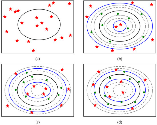
Figure 1.
Schematic diagram of evolution of SAGA.
Evidently, it is very difficult, even impossible, to generate a solution that is located exactly on the equality constraint by randomly initializing the population. For inequality constraints from the conversion of equation constraints, is used to distinguish feasible and infeasible solutions. The feasible region is transformed from a line to an area, but a small positive number means this area is relatively narrow, which leads to a larger popsize required to create the possibility of at least one solution being located in the feasible region after randomly initializing the population. Contrarily, a larger cannot be used in order to guarantee higher computation accuracy. While infeasible solutions are not useless, a better solution may be produced by the combination of a feasible solution and an infeasible solution, two feasible solutions or two infeasible solutions.
The successive approximation strategy of SAGA has a dynamically changing tolerance error of constraints. In the preliminary stage of evolution, a relatively large is given, which makes it very easy for the randomly initialized population to include several feasible solutions, and better solutions can be generated based on these temporary feasible solutions. Then, gradually decreases with the iterations. Finally, reaches the precision required. The whole progress is shown in Figure 1; green points and red stars represent feasible and infeasible solutions, respectively, the area between the two blue rings represents the current temporary feasible region after the conversion of equality constraint and the gray rings represent the boundaries of the temporary feasible regions of other generations. From (b) to (d) in Figure 1, gradually decreases, the temporary feasible region gradually shrinks and all solutions gradually approach the original equation constraint.
Considering that the maximum number of generations is relatively large, it is too cumbersome to operate if is updated after every evolution. Meanwhile, the temporary feasible region shrinking too rapidly may lead to the loss of feasible solutions, so is recommended to be 0.8 times the previous value after every five generations.
3.3. Three-Stages Evolution of SAGA
For the sake of making full use of all solutions, a new population of SAGA is composed of three parts, including the individuals evolving from two feasible solutions (the first part), a feasible and an infeasible solution (the second part) and two infeasible solutions (the third part). In the meantime, the whole evolution progress is divided into three stages including the first third, the middle third and the last third of the generations.
The number of feasible solutions in the solutions generated by randomly initializing the population is very small, and the preliminary stage of evolution is more likely to produce feasible solutions by evolution from infeasible solutions, which is easily found in Figure 1, so the second and third parts account for a larger proportion of the evolution. As iterations go on, the number of feasible solutions gradually increases. The algorithm is also likely to produce feasible solutions by evolution from feasible solutions, so the proportion of the first part in the total evolutionary population gradually increases and the proportion of the third part gradually decreases. In the later stage of evolution, there are many feasible solutions, so the proportion of the first part in the total evolutionary population further increases and the proportion of the third part further decreases (set as zero in the paper). The proportions of every part in different stages are set as shown in Table 1.

Table 1.
The proportion of individuals produced by each part in different stages.
3.4. The Whole Progress of SAGA
SAGA is still mainly composed of population initialization, judgments, iterations, updates and evaluations. Simple and efficient real encoding is adopted in SAGA.
When initializing the population, firstly, two empty sets (set1 and set2) are defined to store feasible and infeasible solutions, respectively. Then, it initializes the population several times, saves the feasible solution obtained after each initialization into set1 until the number of feasible solutions is not less than 10, and only saves the infeasible solution obtained after the last initialization into set2. Finally, it selects set1 as the initial feasible solution set, and randomly selects (popsize—the length of set1) solutions without repeating set2 as the initial infeasible solution set.
The fitness of the individual is calculated according to Equation (13), where is a larger positive number. Roulette wheel selection is adopted in SAGA.
The recombination approach applied by Cai [41] is adopted in SAGA, as shown in Equation (14), where and are two parents, and are two offspring and , , and are four random numbers between zero and one.
The mutation approach applied by Cai [41] is adopted in SAGA as shown in Equation (15), where is a parent, is an offspring, and are the upper and lower bounds of a variable, respectively, is the maximum number of generations and is a random number between zero and one.
During evolution, the solutions are divided into feasible and infeasible solutions after each evolution, and they are extended to the feasible and infeasible solution sets of the last evolution, respectively, so the lengths of set1 and set2 are larger. In order to prevent many similar feasible solutions from appearing too early, which may cause the algorithm to converge prematurely to an imprecise feasible solution, three upper limits on the number of feasible solutions involved in evolution are given in the three stages, as shown in Table 2. For example, in the first stage, if the length of set1 is less than 0.4 times the popsize, all feasible solutions in set1 are involved in the next evolution, and the (popsize—the length of set1) best infeasible solutions in set2 are involved in the next evolution; contrarily, if the length of set1 is more than 0.4 times the popsize, the (0.4 times the popsize) best feasible solutions in set1 are involved in the next evolution, and the (popsize—0.4 times the popsize) best infeasible solutions in set2 are involved in the next evolution, similarly to other stages. A feasible solution determines whether it is good or bad based on the fitness of itself, and an infeasible solution determines whether it is good or bad based on its constraint violation.
Table 2.
The upper limits on the number of feasible solutions involved in evolution.
Finally, all individuals of every generation are re-divided into feasible and infeasible solutions by using the target precision. If feasible solutions exist, the one with the largest fitness is selected as the best individual of the current generation. If no feasible solution exists, the one with the least constraint violation is selected as the best individual of the current generation. The complete process of SAGA is as shown in Figure 2.
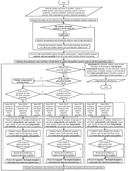
Figure 2.
The flowchart of SAGA.
4. Mathematical Tests and Results of SAGA
Ten nonlinear optimization benchmarks including five problems with an equality constraint and five problems with an inequality constraint were utilized to evaluate the performance of SAGA. All the scripts were written in Python and all the tests were conducted on an Intel Core i7-11370H 3.30GHz machine with 16 GB RAM and single thread under Win10 platform.
4.1. Benchmarks
Five benchmarks with an equality constraint were marked as f1, f2, f3, f4 and f5, and five benchmarks with an inequality constraint were marked as f6, f7, f8, f9 and f10. in f5 was set as 10 in the paper. The mathematical description and optimums of the ten benchmarks are presented in Table 3.
Table 3.
The mathematical expressions of ten benchmarks.
The contour lines or surfaces of the objectives and feasible regions of the decision variables of the ten benchmarks were plotted with Matplotlib and Mayavi. In Figure 3, the optimum of every problem is marked with a red point, of which the corresponding decision variables are also marked in a red transparent box. For f5, makes the problem visible. It is important to note that the figure drawn for f3 is the image of the objective and constraint. The contour surfaces of f9 and f10 are three-dimensional, so the feasible regions are not marked to be observed more visually. Meanwhile, only half of the contour surfaces of f10 are drawn. Furthermore, most optimums of the ten benchmarks are located on the tangent points (tangent planes) of the contour lines (contour surfaces) and feasible regions.
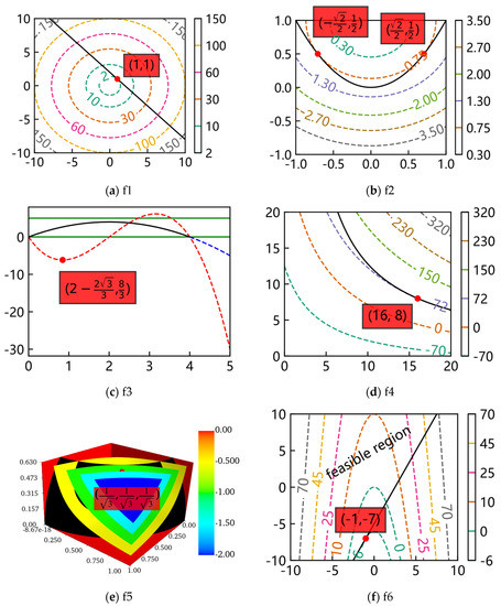
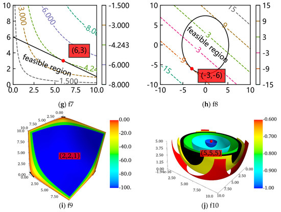
Figure 3.
The contour lines or surfaces and feasible regions of the ten benchmarks.
4.2. Simulation Settings
To explore the appropriate popsize of SAGA to solve the problems well, the popsize of 200, 300, 400 and 500, respectively, was used to run the scripts. In order to obtain more than 10 feasible solutions in a short time in continuous initialization, the popsize used in the initialization was set as a slightly larger number, which was 500 for most of the problems in the paper. The value of in the penalty factor was set as 7. The probability of recombination and mutation were set as 0.65 and 0.05. The maximum number of generations was set as 100. The initial tolerance error was set as 0.1, , so the final tolerance error was set as 0.001. The stop criterion was that the maximum number of generations were reached.
All scripts of SAGA were run 30 times consecutively and the results were recorded.
4.3. Simulation Results
The best result of the 30 runs is defined as the one with the least constraint violation, and the worst result is that with the largest constraint violation. The results and time consumption with different popsizes are shown in Table 4 and Table 5, including the best, worst, mean and standard deviation (SD) of the objectives; the minimum, maximum and mean of the constraint violation; the minimum, maximum and mean errors of the objectives; and the minimum, maximum and mean of the time consumption.
Table 4.
The objective and constraint violation of 30 runs.
Table 5.
The error and time consumption of 30 runs.
The optimum is located on the bound of the constraint for f1 to f9, and it is located in the constraint for f10. In general, for most problems, when the popsize increases, the best and worst values of the objectives of the 30 runs change slightly. In reality, the means of the 30 runs do not mean much because the objective of a solution with a large constraint violation may be closer to the theoretical optimum. The results also demonstrate that the optimums of the 30 runs have small standard deviations; in other words, the proposed SAGA performs with great robustness. Correspondingly, the relevant information of the constraint violation of a solution is more crucial, which directly determines the quality of a solution. The largest constraint violation of ten problems is 0.010938, the others are accurate to at least three decimal fractions.
The tolerance error of the constraint violation and the accuracy of the objective are taken into account at the same time. Then, the appropriate popsize for each problem is found as the bolded texts in Table 4. For the problems with an equality constraint, the suitable popsize is 300 for f1, 200 for f2 and f3, and 400 for f4 and f5. For the problems with an inequality constraint, the suitable popsize is 200 for f6 to f10, which guarantees that the constraint violation can be accurate to three fractions and the objective can be accurate to two fractions.
The errors of the objectives and time consumption corresponding to the appropriate popsize are bolded in Table 5.
All errors corresponding the appropriate popsize listed in Table 5 are very small. For the problems with an equality constraint, SAGA takes an average time of 4.73, 2.31, 0.78, 2.84 and 3.27 s to search for the optimums. For the problems with an inequality constraint, SAGA takes an average time of 0.73, 0.72, 0.75, 0.77 and 0.84 s to search for the optimums. To sum up, SAGA solves the problems with an equality constraint in 5 s and with an inequality constraint in 1 s.
For each problem with the appropriate popsize, the decision variables corresponding to the best and worst constraint violation of 30 runs are presented in Table 6. The decision variables of the best and worst of the 30 best individuals simulated are very close to the theoretical solution, which proves the effectiveness and reliability of SAGA once again.
Table 6.
Decision variables corresponding to the best and worst results.
4.4. Evolution Figures
In order to show the entire evolution process of SAGA more intuitively, for each problem with the appropriate popsize, the evolution processes of the best and worst objectives and corresponding constraint violations of 30 runs are plotted as shown in Figure 4 and Figure 5. For example, SAGA-300-B in a figure means the propriate popsize is 300 and the evolution shown in the figure is the best one of the 30 runs; similarly, W means it is the worst one of the 30 runs.
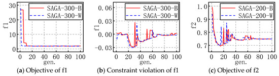
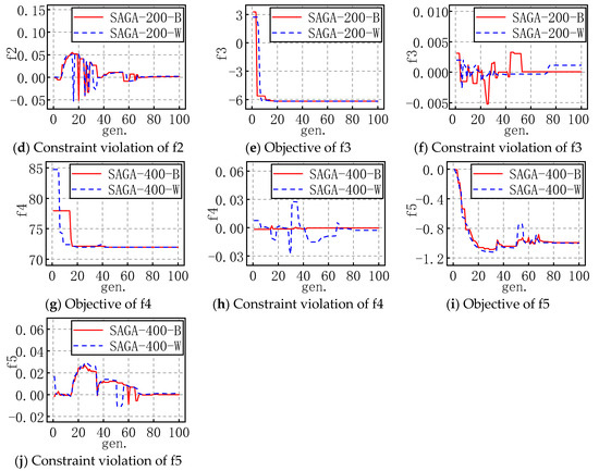
Figure 4.
The evolution figures for f1 to f5.
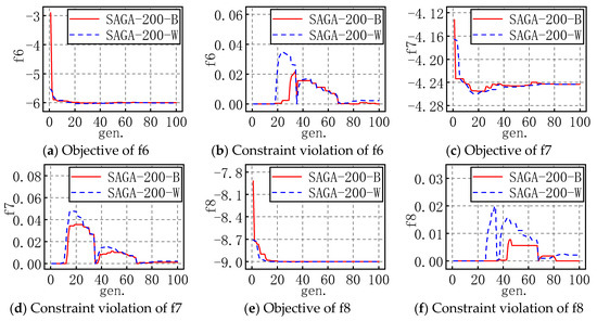
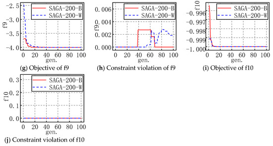
Figure 5.
The evolution figures for f6 to f10.
For the problems with an equality constraint, the results show that the objective fluctuates in the early stages of evolution and gradually levels off in the late stages. The general tendency is that SAGA converges with iterations. Refer to the evolution progress of constraint violation; it is easy to see the phenomenon in which the constraint violation constantly oscillates near zero in the early stages and converges to zero at last, which indicates that SAGA is searching for better and better optimums near the bound of the equality constraint. The above results prove once again that the successive approximation strategy of SAGA is highly efficient.
For the problems with an inequality constraint, the feasible region is an area, not a line, which makes searching for some feasible solutions much easier, so the objective fluctuates slightly in the early stages of evolution and gradually levels off in the late stages. Similarly, SAGA converges with iterations in general. The constraint violation is not less than zero, and it gradually trends towards zero in fluctuations. In actuality, constraint violation may also be less than zero in the evolution, considering the corresponding solution satisfies the inequality constraint, so the constraint violation is set as zero in the figure above. These results also demonstrate that the solutions are more and more accurate and SAGA is highly efficient.
Moreover, combined with the evolution figures of the objectives and constraint violation, it is evident that SAGA converges to an acceptable solution before the maximum number of generations is reached.
Finally, on behalf of the optimization problems with an equality constraint and an inequality constraint, the scripts of f4 and f7 with a popsize of 200 were run once again and the distributions of the population during evolution were plotted to observe the convergence progress of SAGA. Only the distributions of the first, sixth, twelfth, twentieth, fiftieth and hundredth generations are shown in Figure 6 and Figure 7 to describe the process briefly, where the orange pluses represent all individuals of the current generation, the green star represents the best individual of the current generation and the red point represents the theoretical optimum.
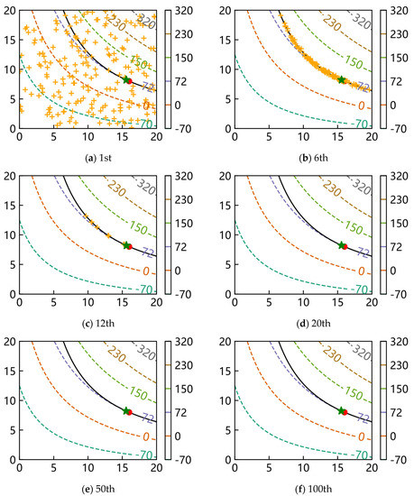
Figure 6.
The distributions of population for f4.
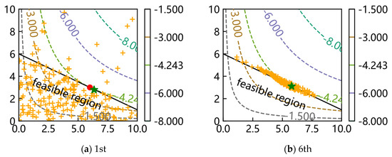
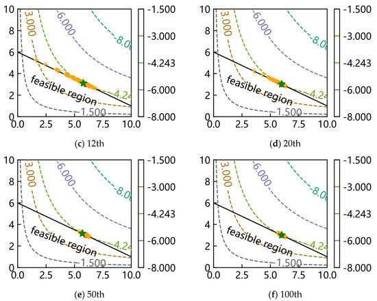
Figure 7.
The distributions of population for f7.
The results show that all individuals are randomly distributed discretely in the whole design space at first, and they gradually move to the bound of constraint with iterations. Most individuals are near the bound after the sixth generation; in other words, SAGA starts to search for a better solution along the bound which satisfies the constraint better afterwards. In the end, all individuals collect near the theoretical optimum. These results again prove that SAGA solves the problems quickly and efficiently.
What is different from Figure 6 is that the feasible region is an area; in the early stages, most individuals are distributed in the feasible region. Other conclusions are consistent with the above.
5. Comparison with the Improved DPGA
Next, the improved dual-population genetic algorithm (IDPGA) was utilized for comparing the performance of SAGA, and the computing platform was consistent with the above. Two improved strategies, including a random dynamic immigration operator and keeping the best individuals, were adopted. Different popsizes and iterations were used for equality constraint problems. The popsize and iteration were taken as 100 for inequality constraint problems. Finally, the tolerance error for equality constraint was set as 0.01.
5.1. Simulation Results of IDPGA
Similarly, the results of 30 runs about objective, constraint violation, error, time consumption and decision variable are listed in Table 7, Table 8 and Table 9.
Table 7.
The objective and constraint violation of 30 runs.
Table 8.
The error and time consumption of 30 runs.
Table 9.
Decision variables corresponding to the best and worst results.
For equality constraint problems, IDPGA behaves better with a larger popsize or iteration. For inequality constraint problems, IDPGA reaches satisfying solutions with a small popsize and iteration. The constraint violation of all results is less than the set value (0.01). Similarly, IDPGA also performs with great robustness. IDPGA takes less than 0.7 s for equality constraint problems and less than 0.1 s for inequality constraint problems to search for the optimums, and the decision variables are close to the theoretical solutions.
5.2. Evolution Figures of IDPGA
The evolution processes of the best and worst result with the appropriate popsize and iteration are plotted in Figure 8 and Figure 9. For example, IDPGA-B in a figure means the evolution shown in the figure is the best one of the 30 runs; similarly, W means it is the worst one of the 30 runs.
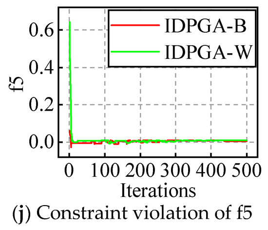
Figure 8.
The evolution figures for f1 to f5.
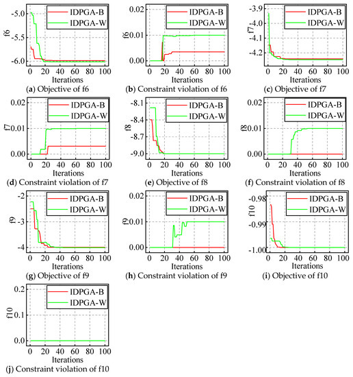
Figure 9.
The evolution figures for f6 to f10.
For ten constraint problems, the results show that the objective does not fluctuate in the early stages, but follows one direction and gradually converges to the optimum. Similarly, the constraint violation oscillates in the early stages and converges near zero at last.
5.3. Comparison of Two Algorithms
In order to compare two algorithms, the best and worst results corresponding to the appropriate popsize and iteration are selected, whose error and constraint violation are shown in Figure 10. Apparently, SAGA can obtain a more precise solution and violate the constraint less than IDPGA. However, combined with the above, IDPGA takes much less time to search than SAGA.
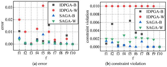
Figure 10.
Comparison of error and constraint violation.
5.4. An Engineering Problem
An engineering optimization problem was solved by two algorithms. The problem is to minimize the weight of a stepped cantilever beam under a vertical concentrated force, as shown in Figure 11. The constraint is the upper limit on the vertical displacement of the free end. The thickness of each element is supposed to be constant, and the decision variables are the width of each element. The mathematical expression is shown in Equation (16).
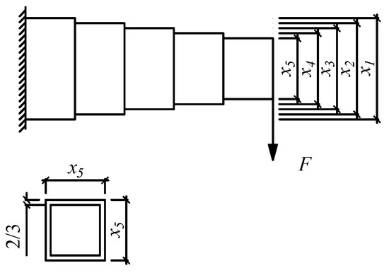
Figure 11.
The diagram of a stepped cantilever beam.
Table 10.
The objective and constraint violation of 30 runs.
Table 11.
The time consumption of 30 runs.
If a constraint is required to be strictly satisfied, IDPGA obtains a best value of 1.3440 and SAGA obtains 1.3398. In reference [42], eight algorithms achieved the best values shown in Table 12. From our findings, SAGA obtains a better value and it also obtains a satisfying value. If the constraint is relaxed appropriately, IDPGA can obtain a value of 1.3344, which can be acceptable in engineering. Furthermore, IDPGA solves the problem much faster than SAGA.
Table 12.
The best objective of 8 algorithms.
6. Conclusions
A new algorithm named the successive approximation genetic algorithm (SAGA) has been proposed by introducing several strategies. After solving a series of mathematic and engineering problems and comparing it with nine other algorithms, we proved that SAGA is highly accurate and effective in solving optimization problems with a constraint, but with a high time cost. In the future, there are several ways in which to improve SAGA. One aspect is to speed up the searching process of SAGA. We are trying to combine the advantages of SAGA and particle swarm optimization to greatly improve its solving efficiency. On the other hand, as seen in Table 1, the proportion of individuals of each part in each stage is determined artificially after trial calculation. Although the results of the problems in the paper are all satisfying, there is no doubt that the proportion of individuals needs to be evaluated in detail in the future. Most engineering problems have many constraints, so another aspect is to extend SAGA to solving optimization problems with multiple, even many, constraints. In this case, if the equality constraints are not properly scaled, the algorithm may easily fall into local optimal even stagnation, which is the direction we are currently exploring.
Author Contributions
Formal analysis, X.X.; Investigation, H.L.; Methodology, Z.C.; Software, X.X.; Supervision, Z.C.; Validation, H.L.; Visualization, Z.C.; Writing—original draft, X.X.; Writing—review and editing, H.L. All authors have read and agreed to the published version of the manuscript.
Funding
The research was under the support of the National Key R&D Program of China (2019YFD1101005).
Data Availability Statement
All scripts of algorithms were completed in Python and all contours were plotted with Matplotlib and Mayavi. Some or all data, models or code that support the findings of this study are available from the corresponding author upon reasonable request.
Conflicts of Interest
On behalf of all authors, the corresponding author states that there are no conflicts of interest.
References
- Ashtari, P.; Barzegar, F. Accelerating fuzzy genetic algorithm for the optimization of steel structures. Struct. Multidiscip. Optim. 2012, 45, 275–285. [Google Scholar] [CrossRef]
- Oskouei, A.V.; Fard, S.S.; Aksogan, O. Using genetic algorithm for the optimization of seismic behavior of steel planar frames with semi-rigid connections. Struct. Multidiscip. Optim. 2012, 45, 287–302. [Google Scholar] [CrossRef]
- Kers, J.; Majak, J.; Goljandin, D.; Gregor, A.; Malmstein, M.; Vilsaar, K. Extremes of apparent and tap densities of recovered GFRP filler materials. Compos. Struct. 2010, 92, 2097–2101. [Google Scholar] [CrossRef]
- Majak, J.; Pohlak, M. Decomposition method for solving optimal material orientation problems. Compos. Struct. 2010, 92, 1839–1845. [Google Scholar] [CrossRef]
- Wang, X.; Yeo, C.S.; Buyya, R.; Su, J. Optimizing the makespan and reliability for workflow applications with reputation and a look-ahead genetic algorithm. Future Gener. Comput. Syst. 2011, 27, 1124–1134. [Google Scholar] [CrossRef]
- Majak, J.; Pohlak, M.; Eerme, M.; Velsker, T. Design of car frontal protection system using neural networks and genetic algorithm. Mechanika 2012, 18, 453–460. [Google Scholar] [CrossRef]
- Qiu, Q.; Cui, L.; Gao, H.; Yi, H. Optimal allocation of units in sequential probability series systems. Reliab. Eng. Syst. Saf. 2018, 169, 351–363. [Google Scholar] [CrossRef]
- Yang, A.; Qiu, Q.; Zhu, M.; Cui, L.; Chen, W.; Chen, J. Condition-based maintenance strategy for redundant systems with arbitrary structures using improved reinforcement learning. Reliab. Eng. Syst. Saf. 2022, 225, 108643. [Google Scholar] [CrossRef]
- Holland, J.H. Adaptation in Natural and Artificial Systems; University of Michigan Press: Ann Arbor, MI, USA, 1975. [Google Scholar]
- Kirkpatrick, S.; Gelatt, C.D.; Vecchi, M.P. Optimization by simulated annealing. Science 1983, 220, 671–680. [Google Scholar] [CrossRef]
- Kennedy, J.; Eberhart, R. Particle swarm optimization. In Proceedings of the ICNN’95—International Conference on Neural Networks, Perth, WA, Australia, 27 November–1 December 1995; Volume 4, pp. 1942–1948. [Google Scholar]
- Hopfield, J.J. Neural networks and physical systems with emergent collective computational abilities. Proc. Natl. Acad. Sci. USA 1982, 79, 2554–2558. [Google Scholar] [CrossRef]
- Colorni, A.; Dorigo, M.; Maniezzo, V. Distributed optimization by ant colonies. In Proceedings of the First European Conference on Artificial Life, Paris, France, 11–13 December 1991; pp. 134–142. [Google Scholar]
- Li, X.L.; Shao, Z.J.; Qian, J.X. An optimizing method based on autonomous animats: Fish-swarm algorithm. Syst. Eng.—Theory Pract. 2002, 22, 32–38. (In Chinese) [Google Scholar]
- Yang, X.-S. Nature-Inspired Metaheuristic Algorithms; Luniver Press: Beckington, UK, 2010. [Google Scholar]
- Yang, X.-S.; Deb, S. Cuckoo search via Lévy flights. In Proceedings of the 2009 World Congress on Nature & Biologically Inspired Computing (NaBIC), New Delhi, India, 9–11 December 2009; IEEE: Piscataway, NJ, USA, 2009; pp. 210–214. [Google Scholar]
- Homaifar, A.; Qi, C.X.; Lai, S.H. Constrained Optimization via Genetic Algorithms. Simulation 1994, 62, 242–253. [Google Scholar] [CrossRef]
- Hoffmeister, F.A.; Sprave, J. Problem-Independent Handling of Constraints by Use of Metric Penalty Functions. In Evolutionary Programming; MIT Press: Cambridge, MA, USA, 1996. [Google Scholar]
- Kuri, A.; Quezada, C. A universal eclectic genetic algorithm for constrained optimization. In Proceedings of the 6th European Congress on Intelligent Techniques & Soft Computing, EUFIT’98, Aachen, Germany, 7–10 September 1998. [Google Scholar]
- Joines, J.A.; Houck, C.R. On the use of non-stationary penalty functions to solve nonlinear constrained optimization problems with GA’s. In Proceedings of the First IEEE Conference on Evolutionary Computation, IEEE World Congress on Computational Intelligence, Orlando, FL, USA, 27–29 June 1994; Volume 2, pp. 579–584. [Google Scholar]
- Kazarlis, S.; Petridis, V. Varying Fitness Functions in Genetic Algorithms: Studying the Rate of Increase of the Dynamic Penalty Terms; Springer: Berlin/Heidelberg, Germany, 1998; pp. 211–220. [Google Scholar]
- Michalewicz, Z.; Attia, N. Evolutionary Optimization of Constrained Problems. In Evolutionary Optimization of Constrained Problems; Springer: Berlin/Heidelberg, Germany, 1994. [Google Scholar]
- Carlson, S.E.; Shonkwiler, R. Annealing a genetic algorithm over constraints. In Proceedings of the SMC’98 Conference Proceedings, 1998 IEEE International Conference on Systems, Man, and Cybernetics (Cat. No.98CH36218), Urbana, IL, USA, 14 October 1998; Volume 4, pp. 3931–3936. [Google Scholar]
- Smith, A.E.; Tate, D.M. Genetic Optimization Using a Penalty Function. In Proceedings of the 5th International Conference on Genetic Algorithms, Urbana-Champaign, IL, USA, 17–21 July 1993; Morgan Kaufmann Publishers Inc.: Burlington, MA, USA, 1993; pp. 499–505. [Google Scholar]
- Coit, D.W.; Smith, A.E. Penalty guided genetic search for reliability design optimization. Comput. Ind. Eng. 1996, 30, 895–904. [Google Scholar] [CrossRef]
- Hadj-Alouane, A.B.; Bean, J.C. A Genetic Algorithm for the Multiple-Choice Integer Program. Oper. Res. 1997, 45, 92–101. [Google Scholar] [CrossRef]
- Deb, K. An efficient constraint handling method for genetic algorithms. Comput. Methods Appl. Mech. Eng. 2000, 186, 311–338. [Google Scholar] [CrossRef]
- Shang, W.F.; Zhao, S.D.; Shen, Y.J. A flexible tolerance genetic algorithm for optimal problems with nonlinear equality constraints. Adv. Eng. Inform. 2009, 23, 253–264. [Google Scholar] [CrossRef]
- Li, X.; Du, G. Inequality constraint handling in genetic algorithms using a boundary simulation method. Comput. Oper. Res. 2012, 39, 521–540. [Google Scholar] [CrossRef]
- Montemurro, M.; Vincenti, A.; Vannucci, P. The Automatic Dynamic Penalisation method (ADP) for handling constraints with genetic algorithms. Comput. Methods Appl. Mech. Eng. 2013, 256, 70–87. [Google Scholar] [CrossRef]
- Liang, X.M.; Qin, H.Y.; Long, W. Genetic Algorithm for Solving Constrained Optimization Problem. Comput. Eng. 2010, 36, 147–149. (In Chinese) [Google Scholar]
- Garcia, R.D.; de Lima, B.; Lemonge, A.C.D.; Jacob, B.P. A rank-based constraint handling technique for engineering design optimization problems solved by genetic algorithms. Comput. Struct. 2017, 187, 77–87. [Google Scholar] [CrossRef]
- Miettinen, K.; Makela, M.M.; Toivanen, J. Numerical comparison of some penalty-based constraint handling techniques in genetic algorithms. J. Glob. Optim. 2003, 27, 427–446. [Google Scholar] [CrossRef]
- Yuan, Q.; He, Z.Q.; Leng, H.N. A hybrid genetic algorithm for a class of global optimization problems with box constraints. Appl. Math. Comput. 2008, 197, 924–929. [Google Scholar] [CrossRef]
- Chootinan, P.; Chen, A. Constraint handling in genetic algorithms using a gradient-based repair method. Comput. Oper. Res. 2006, 33, 2263–2281. [Google Scholar] [CrossRef]
- Lin, F.T. A genetic algorithm for linear programming with fuzzy constraints. J. Inf. Sci. Eng. 2008, 24, 801–817. [Google Scholar]
- Hassanzadeh, R.; Khorram, E.; Mahdavi, I.; Mahdavi-Amiri, N. A genetic algorithm for optimization problems with fuzzy relation constraints using max-product composition. Appl. Soft Comput. 2011, 11, 551–560. [Google Scholar] [CrossRef]
- Abdul-Rahman, O.A.; Munetomo, M.; Akama, K. An adaptive parameter binary-real coded genetic algorithm for constraint optimization problems: Performance analysis and estimation of optimal control parameters. Inf. Sci. 2013, 233, 54–86. [Google Scholar] [CrossRef]
- Tsai, S.C.; Fu, S.Y. Genetic-algorithm-based simulation optimization considering a single stochastic constraint. Eur. J. Oper. Res. 2014, 236, 113–125. [Google Scholar] [CrossRef]
- Zhan, S.C. Genetic Algorithm for Constrained Optimization Problems Which is Based on the Annealing Infeasible Degree. J. Basic Sci. Eng. 2004, 12, 299–304. (In Chinese) [Google Scholar]
- Cai, H.L. Research and Application of Penalty Funciton Method in Constrained Optimization. Master’s Thesis, East China Normal University, Shanghai, China, 2015. (In Chinese). [Google Scholar]
- Zhao, W.; Wang, L.; Mirjalili, S. Artificial hummingbird algorithm: A new bio-inspired optimizer with its engineering applications. Comput. Methods Appl. Mech. Eng. 2022, 388, 114194. [Google Scholar] [CrossRef]


Disclaimer/Publisher’s Note: The statements, opinions and data contained in all publications are solely those of the individual author(s) and contributor(s) and not of MDPI and/or the editor(s). MDPI and/or the editor(s) disclaim responsibility for any injury to people or property resulting from any ideas, methods, instructions or products referred to in the content. |
© 2023 by the authors. Licensee MDPI, Basel, Switzerland. This article is an open access article distributed under the terms and conditions of the Creative Commons Attribution (CC BY) license (https://creativecommons.org/licenses/by/4.0/).