Nonlinear Dynamics of Perturbations of a Plane Potential Fluid Flow: Nonlocal Generalization of the Hopf Equation

Abstract

In this paper, we analytically study the two-dimensional unsteady irrotational flow of an ideal incompressible fluid in a half-plane whose boundary is assumed to be a linear sink. It is shown that the nonlinear evolution of perturbations of the initial uniform flow is described by a one-dimensional integro-differential equation, which can be considered as a nonlocal generalization of the Hopf equation. This equation can be reduced to a system of ordinary differential equations (ODEs) in the cases of spatially localized or spatially periodic perturbations of the velocity field. In the first case, ODEs describe the motion of a system of interacting virtual point vortex-sinks/sources outside the flow domain. In the second case, ODEs describe the evolution of a finite number of harmonics of the velocity field distribution; this is possible due to the revealed property of the new equation that the interaction of initial harmonics does not lead to generation of new ones. The revealed reductions made it possible to effectively study the nonlinear evolution of the system, in particular, to describe the effect of nonlinearity on the relaxation of velocity field perturbations. It is shown that nonlinearity can significantly reduce the relaxation rate by more than 1.5 times.

1. Introduction

The Hopf (Burgers-Hopf) equation [1,2]

$$u_t+u{u}_x=0$$

(1)

is the simplest model in fluid mechanics. It has the meaning of the transport equation for the fluid velocity $u(x,t)$, where $t$ is the time, $x$ is the coordinate, $u_t$ and $u_x$ are the corresponding partial derivatives. This equation arises, for example, when studying the one-dimensional (1D) motion of a gas of noninteracting particles: the 1D Euler equation in the absence of any forces. The nonlinear term of the Hopf equation is a characteristic nonlinearity that occurs in almost any problem of fluid mechanics.

The Hopf equation is easily integrated by the method of characteristics. Its solution is defined implicitly by the formula $u=u_0(x-ut)$ where $u_0(x)=u(x,0)$. The solution exists only for a finite time, being destroyed as a result of the wave breaking. The Hopf equation corresponds to the dispersionless limit of the Burgers, Korteweg-de Vries, and Benjamin–Ono equations. The presence of linear dispersion terms in these equations suppresses the wave breaking process, ensuring the existence of solutions at all times $t>0$.

In the two-dimensional (2D) case, where there are two $x$- and $y$-components of the velocity, $u$ and $v$, respectively, the complex analogue of the Hopf equation

$$U_t+U{U}_z=0$$

(2)

can be applied to describe unsteady potential flows of an incompressible fluid with a free surface [3,4,5]. Here $U=u-iv$ is the complex velocity, which is an analytic function of the complex variable $z=x+iy$ (see also works [6,7,8] and references therein). Equation (2) turns out to be compatible with the 2D Euler equations

$$u_t+u{u}_x+v{u}_y=-p_x/\rho$$

$$v_t+u{v}_x+v{v}_y=-p_y/\rho$$

if the pressure $p$ is related to the velocity component $v$ by the formula $p=-\rho v^2$ (here $\rho$ is the fluid density). The free fluid boundary corresponds to the condition $p=0$ [5]. The complete integrability of the Hopf Equation (2) made it possible to construct a number of nontrivial examples of 2D flows of a fluid with a free surface in the absence of the gravitational force and capillarity. Solutions of the complex Hopf equation are destroyed in a finite time; the analyticity of the function $U$ is violated in the flow domain. This leads to the formation of various types of singularities (depending on initial conditions) on the free surface such as cusps, droplets, and bubbles [5,9,10]. Note that works [11,12] study plane potential flows with a free boundary described by the modified complex Hopf equation

$$U_t+e^{i\gamma }U{U}_z=0,$$

(3)

where $\gamma$ is a real constant. Equation (3) can be reduced to the form (2) by replacing $U\to e^{-i\gamma }U$.

In [13,14], when analyzing the 2D inertial motion of a deep fluid with a free surface in the absence of external forces and capillarity, the following integro-differential equation has been derived in the weakly nonlinear approximation:

$$u_t+u{u}_x-H[u] H[u_x ]=0,$$

(4)

where $H$ stands for the Hilbert transform with respect to $x$ (see Section 3). The nonlocal Equation (4) is transformed into the complex Hopf Equation (2) by introducing the complex velocity $U=u-iH[u]$.

The equation

$$u_t+u{u}_x-H[u] H[u_x ]=-VH[u_x ]$$

(5)

with the nonlinear part coinciding with that of Equation (4), where $V$ is a constant, arose in the study of the instability of the boundary of a conducting liquid in an external electric field [15], as well as of the Kelvin–Helmholtz instability of the interface between two fluids with strongly different densities [16] (compare with [17]). In terms of the complex velocity, it rewrites as

$$U_t+U{U}_x=-iV{U}_x,$$

which differs from the Hopf Equation (2) by the linear term on the right-hand side (this term can be eliminated by the simple change of variables $U\to U-iV$).

Both Equations (4) and (5), due to their connection with the Hopf equation, describe the formation of singularities at the fluid boundary in a finite time (to be precise, the formation of Moore’s singularities [18]).

In the present paper, when considering a certain 2D flow in the half-plane $-\infty <x<\infty$ and $y\ge 0$, we arrive at the new nonlinear integro-differential equation

$$u_t+u{u}_x+H[u] H[u_x ]=VH[u_x ].$$

(6)

It contains the same terms as Equation (5) but differs from it in the signs of the second nonlinear term and of the linear term on the right-hand side. As a result, it cannot be reduced to the complex Hopf equation and its modifications. Equation (6) has the same symmetries as the Hopf equation, however, as will be shown, it has fundamentally different properties that are closer to those of the Laplacian growth equation [19,20]. This leads to the need to use different methods of integrating the equation and to other properties of its solutions. The solutions remain smooth at all times $t>0$.

The plan of the paper is as follows: Section 2 contains the formulation of the problem where we write down the equations describing the two-dimensional unsteady flow of an incompressible fluid in a half-plane, the boundary of which corresponds to a linear sink. A physical interpretation of such a flow is given. Section 3 derives the key integro-differential Equation (6), which can be considered as a nonlocal generalization of the Hopf equation. Section 4 and Section 5 show that this equation can be reduced to a finite number of ordinary differential equations (ODEs) for the cases of either spatially localized or spatially periodic perturbations of the initial uniform flow. In the first case, ODEs describe the motion of a system of interacting virtual point vortex-sinks/sources outside the flow domain. In the second case, ODEs describe the evolution of a finite number of harmonics of the velocity field distribution. Such a reduction is possible due to the following revealed property of Equation (6): the interaction of initial harmonics does not lead to the generation of new ones. It is demonstrated that the influence of the nonlinearities of Equation (6) leads to a rather complex dynamics of velocity field perturbations. The character of perturbation relaxation described by exact solutions of the problem and by solutions obtained in the linear approximation is compared. It is shown that nonlinearity significantly decreases the relaxation rate. Finally, Section 6 contains some concluding remarks.

2. Formulation of the Problem and Initial Equations

We will consider the following 2D boundary-value problem:

$${\mathsf{\Phi }}_{xx}+{\mathsf{\Phi }}_{yy}=0,\hspace{1em}\hspace{1em}0<y<\infty ,$$

(7)

$${\mathsf{\Phi }}_t+\frac{1}{2} {({\mathsf{\Phi }}_x)}^2+\frac{1}{2} {({\mathsf{\Phi }}_y)}^2=\frac{1}{2} V^2,\hspace{1em}\hspace{1em}y=0,$$

(8)

$${\mathsf{\Phi }}_y\to -V,\hspace{1em}\hspace{1em}y\to \infty ,$$

(9)

where $V>0$ is some constant. These equations describe the irrotational flow of an incompressible liquid in the half-plane $-\infty <x<\infty$ and $y>0$ with the velocity potential $\mathsf{\Phi }(x,y,t)$ (we have $\{u,v\}=\{{\mathsf{\Phi }}_x,{\mathsf{\Phi }}_y\}$ for the $x$- and $y$-components of the velocity vector). The potential $\mathsf{\Phi }$ satisfies the Laplace Equation (7), which is compatible with the non-stationary Bernoulli equation

$${\mathsf{\Phi }}_t+\frac{1}{2} {({\mathsf{\Phi }}_x)}^2+\frac{1}{2} {({\mathsf{\Phi }}_y)}^2=-\frac{p}{\rho }+\Gamma (t),\hspace{1em}\hspace{1em}0<y<\infty ,$$

(10)

where $\rho =\mathrm{const}$ is the fluid density, $p(x,y,t)$ is the pressure, and $\Gamma$ is some function of time arising from the spatial integration of the Euler equations. According to Condition (9), the flow is uniform at infinity $y\to \infty$ and directed along the $y$ axis in the negative direction; $V$ is the absolute value of the velocity of this flow. The fluid flows out of the domain $-\infty <x<\infty$ and $y>0$, crossing its linear boundary $y=0$. We suppose that the pressure along this boundary is constant, $p{|}_{y=0}=p_0=\mathrm{const}$. In view of Equation (10), this boundary condition can be written as

$${\mathsf{\Phi }}_t+\frac{1}{2} {({\mathsf{\Phi }}_x)}^2+\frac{1}{2} {({\mathsf{\Phi }}_y)}^2=-\frac{p_0}{\rho }+\Gamma (t),\hspace{1em}\hspace{1em}y=0.$$

(11)

Using some arbitrariness in determining the velocity potential, we choose $\Gamma =p_0/\rho +V^2/2=\mathrm{const}$, which reduces (11) to the Form (8). It is clear that the uniform flow $\{u,v\}=\{0,-V\}$ gives the trivial, unperturbed solution to the problem. In terms of the velocity potential, this solution is

$$\mathsf{\Phi }=-Vy.$$

(12)

We will be interested in the dynamics of perturbations of this basic flow.

The formulated problem can be considered as describing an upstream flow before a linear sink on the straight line $-\infty <x<\infty$ and $y=0$. For clarity, one can imagine the flow in front of a waterfall. In the upstream region $y>0$, i.e., before the waterfall, we have a plane potential flow of a fluid placed between two horizontal semi-infinite plates; the depth of the fluid layer (it corresponds to the vertical direction in three-dimensional consideration) is much less than the characteristic scale of the flow in the plane $\{x,y\}$. The fluid flows across the plateau $y>0$ towards the cliff edge $y=0$, where the plates end, and then it falls freely (see, for example, [21,22,23]). If we again assume that the flow scale in the plane $\{x,y\}$ is dominant, then we can admit that the pressure is unloaded at the boundary $y=0$ to its atmospheric value $p_0$, which is embedded in Equation (8). Thus, Equations (7)–(9) can be interpreted as a toy model of 2D flow in front of a linear sink/waterfall.

In view of the indicated interpretation of the problem (7)–(9), it must be supplemented with the condition that the liquid cannot flow into the domain $y>0$ through its boundary $y=0$; the $y$-component of the velocity cannot be positive at $y=0$, i.e., $v{|}_{y=0}\le 0$. In terms of the velocity potential $\mathsf{\Phi }$, this corresponds to the kinematic condition in the form of the inequality

$${\mathsf{\Phi }}_y\le 0,\hspace{1em}\hspace{1em}y=0.$$

(13)

Indeed, the fluid falls freely after crossing the boundary $y=0$, so that it cannot subsequently return to the region $y>0$. This immediately leads to Condition (13) for the velocity component normal to the flow boundary.

3. Derivation of the Key Equation

Let us reduce the original 2D problem to a single 1D evolution equation. Considering a uniform flow with the velocity potential $\mathsf{\Phi }=-Vy$ as unperturbed, we introduce the potential perturbation as $\phi =\mathsf{\Phi }+Vy$. Substituting it into (7)–(9), we obtain

$${\phi }_{xx}+{\phi }_{yy}=0,\hspace{1em}\hspace{1em}0<y<\infty ,$$

(14)

$${\phi }_t+\frac{1}{2} {({\phi }_x)}^2+\frac{1}{2} {({\phi }_y)}^2=V{\phi }_y,\hspace{1em}\hspace{1em}y=0,$$

(15)

$${\phi }_y\to 0,\hspace{1em}\hspace{1em}y\to \infty .$$

(16)

It is necessary to eliminate the variable $y$ from these equations. Note that the solution of the two-dimensional Laplace Equation (14) at $y>0$ in view of the condition (16) is given by

$$\phi (x,y,t)=\frac{1}{\pi }{\displaystyle \underset{-\infty }{\overset{+\infty }{\int }}} \frac{y \psi (x^{\prime },t)}{y^2+{(x^{\prime }-x)}^2} d{x}^{\prime },$$

where $\psi (x,t)\equiv \phi {|}_{y=0}$ is the function that specifies the perturbation of the velocity potential at the boundary $y=0$. Differentiating this expression with respect to $y$, we find ${\phi }_y=H[{\psi }_x ]$ at $y=0$, where $H$ is the Hilbert transform with respect to $x$ (the “P.V.” denotes the principal-value integral):

$$H[f(x)]=\frac{1}{\pi } \mathrm{P}.\mathrm{V}. {\displaystyle \underset{-\infty }{\overset{+\infty }{\int }}}\frac{f(x^{\prime })}{x^{\prime }-x} d{x}^{\prime }.$$

As a result, we obtain from (15) the one-dimensional nonlinear evolution equation for the function $\psi (x,t)$, which will be the subject of our further consideration:

$${\psi }_t+\frac{1}{2}{({\psi }_x)}^2+\frac{1}{2}{(H[{\psi }_x ])}^2=VH[{\psi }_x ].$$

(17)

To clarify the notation used in this equation, we can rewrite it in the equivalent form

$${\psi }_t+\frac{1}{2}{({\psi }_x)}^2+\frac{1}{2}{(K[\psi ])}^2=-VK[\psi ],$$

where $K\equiv -{\partial }_{x}H$ is the integral operator with the Fourier transform equal to $\left|k\right|$, i.e., $K[e^{ikx} ]= \left|k\right|e^{ikx}$ (see [14,15,16]).

The obvious difficulty in studying Equation (17) is that it is no longer a partial differential equation, similar to the original Equations (7)–(9), but an integro-differential equation. We also recall that we are not interested in all solutions of Equation (17), but only in those that satisfy the Condition (13), which, in terms of the function $\psi$, can be rewritten as

$$H[{\psi }_x ]\le V.$$

(18)

By differentiating Equation (17) with respect to $x$, we arrive at the following equation for the $x$-component of the velocity at the boundary $y=0$, $u{|}_{y=0}={\psi }_x$:

$$u_t+u{u}_x+H[u] H[u_x ]=VH[u_x ].$$

(19)

It can be considered as a nonlocal generalization of the Hopf equation (see Section 1 for details).

In the linear approximation, Equation (17) turns into the compact equation

$${\psi }_t=VH[{\psi }_x ].$$

(20)

The dispersion relation for (20) can be obtained by substituting $\psi \propto \exp (ikx-i\omega t)$, where $\omega$ is the frequency and $k$ is the wave number. Taking into account the property $H[e^{ikx} ]=i \mathrm{sgn}(k)e^{ikx}$ of the Hilbert transform, we find the simple expression

$$\omega =-iV\left|k\right|.$$

(21)

According to this expression, perturbations decay with the characteristic time $1/(V|k|)$. Such relaxation is obviously due to the fact that perturbations of the velocity field are carried downstream with the velocity $V$, i.e., the linear stability of the unperturbed flow (12) is inherent in the formulation of the problem itself. The relaxation character is determined by the fact that Equation (20) is actually elliptical, that is, it corresponds to one of the branches of the dispersion law ${\omega }^2=-V^2{k}^2$ of the equation ${\psi }_{tt}+V^2{\psi }_{xx}=0$. Note the difference in the character of relaxation processes from those described by the parabolic and hyperbolic heat diffusion equations [24].

The present work is devoted to a large extent to the consideration of how the nonlinear terms of Equation (17) will affect the character of the relaxation of perturbations. First of all, this is important for situations where the perturbations are not small and, therefore, the approximation (20) together with the dispersion law (21) are not applicable. Below we will pay considerable attention to situations where, at the initial moment of time $t=0$ at some point, for example, at $x=0$, the $y$-component of the velocity at the boundary (for convenience we denote it as $v_b(x,t)\equiv v{|}_{y=0}=-V+H[{\psi }_x ]$) is equal to zero: $v_b(0,0)=0$. For instance, one can take the initial velocity distribution in the form

$$v_b(x,0)=-V+\frac{4a^{2}V}{V^2{x}^2+4a^2},$$

(22)

for which $v_b(x,0)\to -V$ at $\left|x\right|\to \infty$ and $v_b(0,0)=0$ (here $a$ is some constant). Such a situation can be considered as the presence of an obstacle in the downflow, which is removed at the moment $t=0$. Then we need to describe the relaxation of the flow to the unperturbed state $\{u,v\}=\{0,-V\}$ taking into account the influence of nonlinear terms in Equation (17). For the initial velocity distribution (22) (the perturbation of the $y$-component of the velocity at $x=0$ is equal to the velocity of the basic flow, taken with the opposite sign), the contribution of linear and nonlinear terms will be comparable.

Let us represent the perturbation of the velocity potential at the boundary in the form

$$\psi ={\psi }^{+}+{\psi }^{-},$$

where ${\psi }^{\pm }$ are analytic continuations of the function $\psi$ into the upper and lower half-planes, respectively, of the complex variable $x$. The functions ${\psi }^{\pm }$ can be written as the actions of the projectors $P^{\pm }=(1\mp iH)/2$ on the function $\psi$: ${\psi }^{\pm }=P^{\pm }[\psi ]$. Due to the property $H[{\psi }^{\pm }]=\pm i{\psi }^{\pm }$ of the Hilbert transform, Equation (17) takes the form

$${\psi }_t^{+}+ {\psi }_t^{-}+2{\psi }_x^{+}{\psi }_x^{-}=iV{\psi }_x^{+}-iV{\psi }_x^{-}.$$

It can be separated into a pair of equations for parts that are analytic in the upper and lower half-planes of the $x$ variable:

$${\psi }_t^{\pm }+2P^{\pm }[{\psi }_x^{+}{\psi }_x^{-}]=\pm iV{\psi }_x^{\pm }.$$

Since the functions ${\psi }^{\pm }$ are complex conjugates, these equations are also complex conjugates. Then it suffices to consider, for instance, only the equation for the function ${\psi }^{+}$, namely

$${\psi }_t^{+}+2P^{+}[{\psi }_x^{+}{\psi }_x^{-}]=iV{\psi }_x^{+}.$$

(23)

The nonlinear part of Equation (23) resembles the well-known Laplacian growth equation (LGE),

$$\mathrm{Im}({\psi }_t^{+}{\psi }_x^{-})=1,$$

which is used for describing the 2D motion of the boundary between two liquids with noticeably different viscosities (Hele-Shaw flow) [25,26,27], evolution of the free surface of a liquid in a gravitational field in the high-Jacobian approximation [28,29], electrostatic aggregation in two dimensions [30], electrohydrodynamic and quantum Kelvin–Helmholtz instabilities of the free surface of liquid helium [31,32], and so on. It is integrable in the sense of the existence of an infinitely large number of exact particular solutions and relation to the dispersionless limit of the integrable Toda hierarchy [33]. LGE can be written in the form

$${\psi }_t^{+}{\psi }_x^{-}-{\psi }_t^{-}{\psi }_x^{+}=2i,$$

or, in order to emphasize the similarity with Equation (23), in the form

$${\psi }_t^{+}+P^{+}[{\psi }_t^{+}{\psi }_x^{-}-{\psi }_t^{-}{\psi }_x^{+}]=-i{\psi }_x^{+},$$

(24)

where we have made the changes ${\psi }^{\pm }={\psi }^{\pm }\pm it+x$ and applied the operator $P^{+}$. A common feature of Equations (23) and (24) is that their nonlinear parts contain only cross terms with respect to the functions ${\psi }^{+}$ and ${\psi }^{-}$ (in other words, they are linear in ${\psi }^{+}$ and ${\psi }^{-}$). This will allow us to apply to Equation (23) a number of techniques [26,27,30,34], which were developed for LGE, and, as a result, to construct spatially localized (Section 4) and spatially periodic (Section 5) solutions of the problem.

4. Spatially Localized Solutions

We are looking for a solution of Equation (23) as a sum of $N$ logarithmic singularities,

$${\psi }^{+}(x,t)={\displaystyle \sum _{j=1}^N{s}_j}\ln \left(x-Z_j(t)\right),$$

(25)

where $s_j$ are complex constants, $Z_j(t)$ are complex functions specifying positions of singularities in the complex plane $x$. Let $Z_j(t)=X_j(t)+i{Y}_j(t)$, where $X_j(t)=Re{Z}_j(t)$ and $Y_j(t)=\mathrm{Im}{Z}_j(t)$. Since ${\psi }^{+}$ must be analytic in the upper half-plane of the variable $x$, all singularities are located in the lower half-plane, i.e., the conditions $Y_j(t)<0$ are valid for all $j=1, 2,\dots , N$. If it becomes $Y_j(t)=0$ at some moment, then the solution will be destroyed. Note that the representation (25) corresponds to a system of moving virtual point vortex-sinks/sources in the region $y<0$, i.e., outside the flow domain. Each singularity in (25) corresponds to a separate spatially localized perturbation of the velocity field.

By substituting (25) into (23) and then expanding the resulting expression into simple fractions (pole decomposition), we get the following system of $N$ ODEs for the motion of singular points:

$$\frac{d}{dt}{Z}_j={\displaystyle \sum _{m=1}^N\frac{2\overline{s_m}}{Z_j-\overline{Z_m}}}-iV,\hspace{1em}\hspace{1em}j=1,2,\dots ,N.$$

(26)

Thus, the analysis of the integro-differential Equation (23) is reduced to the analysis of the ODE system (26), for which a significant number of exact solutions can be found (note that a similar system of ODEs arising from the LGE can be easily integrated).

First, we consider the simplest case of $N=1$, i.e., we look for a solution in the form

$${\psi }^{+}(x,t)=s\ln \left(x-Z(t)\right).$$

(27)

According to (26), the singularity position is described by ODE as

$$\frac{d}{dt}Z=\frac{2\overline{s}}{Z-\overline{Z}}-iV.$$

(28)

Let $s=a+ib$ and $Z(t)=X(t)+iY(t)$. Separating (28) into real and imaginary parts, we arrive at a pair of ODEs

$$\frac{d}{dt}X=-\frac{b}{Y},$$

(29)

$$\frac{d}{dt}Y=-\frac{a}{Y}-V$$

(30)

with the initial conditions $X(0)=X_0$ and $Y(0)=Y_0<0$.

Equation (30) for $Y$ admits the stationary solution

$$Y=Y_{\mathrm{st}}=Y_0=-a/V,$$

(31)

where $a>0$. The corresponding solution to Equation (29) has the form

$$X=(b/a)Vt+X_0,$$

(32)

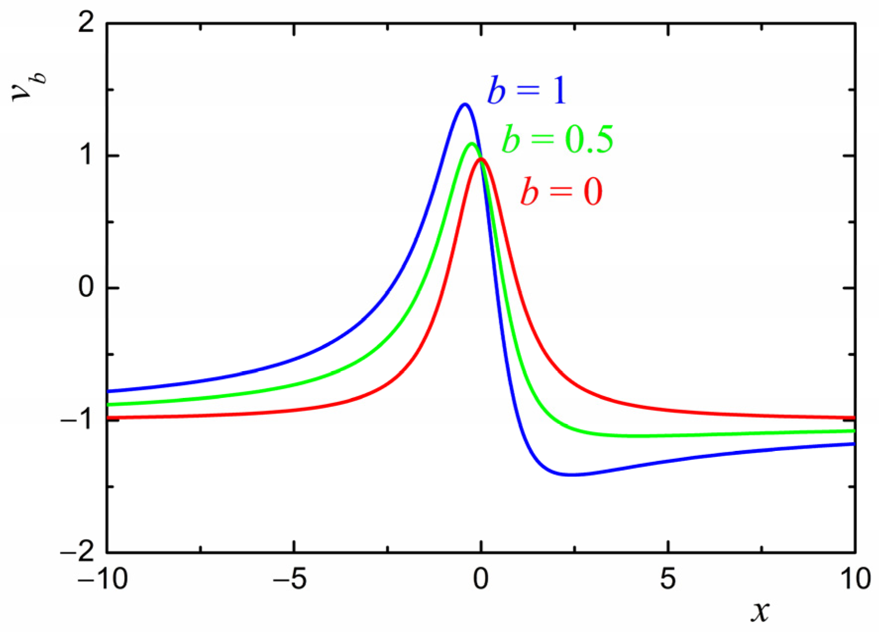
i.e., the singularity moves with constant velocity parallel to the real axis. Such a solution can be interpreted as a soliton solution of Equation (17); however, this exact solution does not make sense in the context of the problem under consideration, since it violates the Condition (18) of non-positivity of the normal velocity at the fluid boundary, $v_b(x,t)\equiv -V+i{\psi }_x^{+}-i{\psi }_x^{-}\le 0$. Indeed, the normal velocity for the representation (27) is given by the expression

$$v_b(x,t)=-V+i\frac{s}{x-Z(t)}-i\frac{\overline{s}}{x-\overline{Z}(t)}=-V-2\frac{b\left(x-X(t)\right)+aY(t)}{{\left(x-X(t)\right)}^2+Y^2(t)}.$$

(33)

For the soliton solutions (31) and (32), the characteristic distributions of the velocity along the boundary are shown in Figure 1. It can be seen that there is always a region of positive velocities, i.e., formally, the fluid flows into the region $y>0$ through the boundary $y=0$, which violates the requirements imposed on possible solutions.

It can be seen from Equation (30) that the singularity always moves away from the real axis for $a\le 0$. For $a>0$, it moves away from the real axis if $Y_0<Y_{\mathrm{st}}$ and approaches it if $Y_0>Y_{\mathrm{st}}$. In the latter case, the solution is destroyed as a result of violation of the condition of analyticity of the function ${\psi }^{+}$ when the singularity reaches the real axis at some finite time $t_c$ with asymptotic behavior $Y\approx -\sqrt{2a(t_c-t)}$. However, such a scenario of the solution destruction has no physical meaning, since when the condition $Y_0>Y_{\mathrm{st}}$ holds, the non-positivity condition for the normal velocity at the fluid boundary is obviously violated (see Figure 1 for $Y_0=Y_{\mathrm{st}}$).

We consider several simple cases that do not violate the condition $v_b\le 0$. Let $a>0$ and $b=0$. According to (33), the distribution of the normal velocity at the boundary is determined by the expression

$$v_b(x,t)=-V-\frac{2aY(t)}{x^2+Y^2(t)}.$$

(34)

In this case, as can be seen from ODE (29), the singularity does not move along the real axis, i.e., $X(t)=X_0=\mathrm{const}$. We choose the following initial conditions: $X_0=0$ and $Y_0=-2a/V$. This gives the initial velocity distribution (22), where the velocity vanishes at a single point at the origin: $v_b(0,0)=0$. As stated in Section 3, such an initial condition corresponds to the situation where there was an obstacle at the boundary $y=0$, which was removed at time $t=0$.

In the linear approximation (i.e., we consider the linearized Equation (20) instead of the original one (17)), ODEs (29) and (30) take the trivial form

$$\frac{d}{dt}X=0,\hspace{1em}\hspace{1em}\frac{d}{dt}Y=-V,$$

i.e., the singularity moves away from the real axis with constant velocity $V$:

$$X_{\mathrm{lin}}(t)=X_0=0,\hspace{1em}\hspace{1em}{Y}_{\mathrm{lin}}(t)=Y_0-Vt= -2a/V-Vt.$$

According to (34), the normal velocity at the center of the perturbation evolves as

$$v_b(0,t)=-V-\frac{2a}{Y(t)}.$$

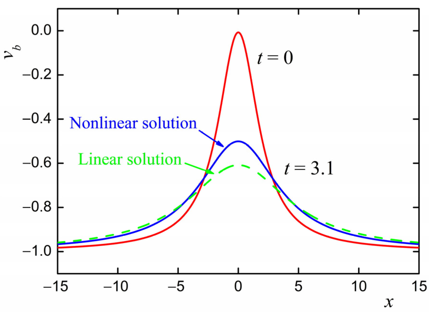
Then, as a result of the linear relaxation of the perturbation, the velocity reaches the value of $-0.5V$ (i.e., half of the unperturbed flow velocity) at the time instant $t_{\mathrm{lin}}=2a/V^2$, when $Y(t_{\mathrm{lin}})= -4a/V$.

Let us consider how nonlinearity will affect the relaxation of the perturbation. The exact solution of the nonlinear Equation (30) is written in implicit form as

$$\frac{Y(t)+2a/V}{V}-\frac{a}{V^2}ln\left(\frac{-a-VY(t)}{a}\right)=-t.$$

The velocity reaches the value of $-0.5V$ at the time instant

$$t_{\mathrm{nl}}=\frac{2a}{V^2}\left(1+ln\sqrt{3}\right).$$

The ratio of the nonlinear and linear relaxation times is

$$t_{\mathrm{nl}}/t_{\mathrm{lin}}=1+ln\sqrt{3}\approx 1.55,$$

i.e., the relaxation proceeds more than one and a half times slower than in the linear approximation. This is demonstrated in Figure 2, which shows the distribution of the normal velocity at the boundary ($v_b$) at the initial moment $t=0$ and at the moment $t=t_{\mathrm{nl}}$ both for the exact solution and for the linear approximation. It can be seen that the influence of nonlinear terms of Equation (17) significantly affects the process of relaxation of the perturbation of the basic fluid flow.

Now let $a=0$ and $b>0$. Then, according to (33), the distribution of the normal velocity at the boundary is determined by the expression

$$v_b(x,t)=-V-2\frac{b\left(x-X(t)\right)}{{\left(x-X(t)\right)}^2+Y^2(t)}.$$

We take the initial conditions $X_0=0$ and $Y_0=-b/V$, which correspond to the initial velocity distribution

$$v_b(x,0)=-V-2\frac{b{V}^{2}x}{V^2{x}^2+b^2}.$$

(35)

According to this expression, at the initial time $t=0$, the velocity vanishes at the only point $x=-b/V$, i.e., $v_b(-b/V,0)=0$ (the red line in Figure 3). Note that this perturbation of the velocity field, in contrast to (22), is not symmetric. This can be associated with a different geometry of the obstacle on the flow path.

The solution of the nonlinear ODEs (29) and (30) describing the singularity motion is

$$X(t)=\frac{b}{V}\ln \left(\frac{b+V^{2}t}{b}\right),\hspace{1em}\hspace{1em}Y(t)=-b/V-Vt.$$

(36)

Trivial equations

$$\frac{d}{dt}X=0,\hspace{1em}\hspace{1em}\frac{d}{dt}Y=-V$$

are the linear analog of ODEs (29) and (30). Their solution has the form

$$X_{\mathrm{lin}}(t)=0,\hspace{1em}\hspace{1em}{Y}_{\mathrm{lin}}(t)=Y(t)=-b/V-Vt.$$

(37)

Figure 3 shows the evolution of the normal velocity at the boundary ($v_b$) corresponding to the exact solution (36) as well as to the linear approximation (37). The relaxation rate of the flow velocity perturbation for this case is the same in linear and nonlinear approximations. The singular point moves away from the real axis at the same velocity. However, linear and nonlinear velocity distributions are noticeably different, which is associated with the displacement of the perturbation along the $x$ axis according to the logarithmic dependence in (36).

Let us now discuss the case $N\ge 2$. In the general case, the corresponding ODEs are non-integrable, and the dynamics of singular points are extremely complex; however, two relatively simple cases, viz. the cases of (i) independent and (ii) collective motion of singularities can be singled out.

The case of independent motion is realized if the interaction between singularities is weak. This, as can be easily seen from ODEs (26), occurs if the conditions

$$\left|Z_j-\overline{Z_m}\right|>>\left|Z_j-\overline{Z_j}\right|,\hspace{1em}\hspace{1em}j\ne m$$

(38)

are satisfied, i.e., singular points are located relative to each other at greater distances than the distances from them to the real axis. In this case, the velocity field perturbations corresponding to the singularities are separated in space and evolve independently of each other according to the solutions described above for $N=1$.

The case of collective motion of singularities is realized when distances between them on the complex plane are much smaller than the distances to the real axis

$$\left|Z_j-Z_m\right|<<\left|Z_j-\overline{Z_j}\right|.$$

(39)

where $j=1,2,\dots ,N$ and $m=1,2,\dots ,N$. Note that these inequalities are not opposite to the inequalities (38).

It is convenient to analyze ODEs (26) using the “center-of-mass” system of coordinates, the origin of which is given by the expression

$$Z(t)=\frac{1}{S}{\displaystyle \sum _{j=1}^N{s}_j{Z}_j(t)},\hspace{1em}\hspace{1em}S={\displaystyle \sum _{j=1}^N{s}_j}.$$

(40)

We put

$$Z_j(t)=Z(t)+\delta Z_j(t),\hspace{1em}\hspace{1em}j=1,2,\dots ,N,$$

(41)

where $\delta Z_j(t)$ are small deviations of the positions of singularities from the position of the “center of mass”. In view of the Definition (40), the following relation

$${\displaystyle \sum _{j=1}^N{s}_j\delta Z_j(t)}=0$$

(42)

holds. By substituting (41) into ODEs (26) and then expanding these equations in power series of small quantities $(\delta Z_j-\overline{\delta Z_m})/(Z-\overline{Z})$, we get, in the main order, the equation of motion of the “center of mass”:

$$\frac{d}{dt}Z=\frac{2\overline{S}}{Z-\overline{Z}}-iV.$$

After the replacement $S\to s$, it will coincide with the equation of motion of a single singularity (28). Its exact implicit solution is

$$\frac{Y(t)-Y_0}{V}-\frac{a}{V^2}ln\left(\frac{a+VY(t)}{a+V{Y}_0}\right)=-t,$$

(43)

$$X(t)=X_0-{\displaystyle \underset{0}{\overset{t}{\int }}\frac{b}{Y(t^{\prime })}d{t}^{\prime }},$$

(44)

where, as before, $Z=X+iY$, $S=a+ib$, $X_0=X(0)$, and $Y_0=Y(0)$.

In the next order of smallness, we obtain linear equations for the deviations $\delta Z_j(t)$,

$$\frac{d}{dt}\delta Z_j=-\frac{1}{{(Z-\overline{Z})}^2}{\displaystyle \sum _{m=1}^{N}2\overline{s_m}(\delta Z_j-\overline{\delta Z_m})},\hspace{1em}\hspace{1em}j=1,2,\dots ,N,$$

or, taking into account the Formulas (40) and (42), the following compact equations:

$$\frac{d}{dt}\delta Z_j=-\frac{2\overline{S}}{{(Z-\overline{Z})}^2}\delta Z_j=\frac{\overline{S}}{2{(\mathrm{Im}Z)}^2}\delta Z_j,\hspace{1em}\hspace{1em}j=1,2,\dots ,N.$$

(45)

Note that the Condition (42) agrees with these equations:

$$\frac{d}{dt}{\displaystyle \sum _{j=1}^N{s}_j\delta Z_j}=-\frac{2\overline{S}}{{(Z-\overline{Z})}^2}{\displaystyle \sum _{j=1}^N{s}_j\delta Z_j}=0.$$

Thus, in the considered approximation, the initial system of Equation (26) is split into independent equations for the quantities $\delta Z_j(t)$, which drastically simplifies its analysis. We introduce the auxiliary time variable

$$\tau ={\displaystyle \int \frac{dt}{2{(ImZ)}^2}}.$$

Then Equation (45) take the simple form

$$\frac{d}{d\tau }\delta Z_j=\overline{S}\delta Z_j,\hspace{1em}\hspace{1em}j=1,2,\dots ,N.$$

Their obvious solutions are

$$\delta Z_j(\tau )=\delta Z_j(0)e^{\overline{S}\tau },\hspace{1em}\hspace{1em}j=1,2,\dots ,N.$$

Hence it is clear that the character of the collective behavior of singularities is determined by the quantity $\overline{S}$. If $\mathrm{R}\mathrm{e}\overline{S}<0$, then singular points converge with time. If $\mathrm{R}\mathrm{e}\overline{S}>0$, then singular points move away from each other. For $\mathrm{R}\mathrm{e}\overline{S}=0$, they rotate around the “center of mass”, which moves according to Solutions (43) and (44).

It can be expected that, in the intermediate case where inequalities (38) or (39) are not satisfied, the dynamics of singularities will be extremely complex and possibly chaotic.

5. Spatially Periodic Solutions

In this section, we will demonstrate the possibility of constructing exact spatially periodic solutions of the problem under consideration. We will look for solutions with the period $2\pi /k$ ($k>0$ is the wave number of the basic harmonic) in the form of a sum of $N+1$ harmonics, including the zero one, with (in the general case) complex amplitudes $A_j$,

$${\psi }^{+}(x,t)=\frac{1}{2}{A}_0(t)+{\displaystyle \sum _{j=1}^N{A}_j(t)e^{ijkx}}.$$

(46)

A remarkable feature of the nonlinear part of Equation (17) (or of Equation (19)) is that it does not generate new harmonics with numbers greater than $N$. By substituting (46) into Equation (23), we arrive at the system of $N+1$ equations for the temporal evolution of the amplitudes $A_j$:

$$\frac{d}{dt}{A}_j=-2k^2{\displaystyle \sum _{m=0}^{N-j}(j+m)m{A}_{j+m}\overline{A_m}}-jkV{A}_j,\hspace{1em}\hspace{1em}j=0, 1, 2,\dots , N.$$

(47)

It is clear that this reduction opens up the possibility of constructing a significant number of exact analytical solutions to the problem.

We restrict ourselves here to a relatively simple special case of $N=2$ with real amplitudes $A_{0,1,2}$. For simplicity, let us take $k=1$ (in which case the wavelength equals $2\pi$). This corresponds to the following representation for the function ${\psi }^{+}$:

$${\psi }_{+}(x,t)=\frac{1}{2}{A}_0(t)+A_1(t)e^{ix}+A_2(t)e^{2ix}.$$

(48)

According to (47), such a substitution leads to the system of three nonlinear ODEs,

$$\frac{d}{dt}{A}_0=-2A_1^2-8A_2^2,$$

(49)

$$\frac{d}{dt}{A}_1=-4A_1{A}_2-V{A}_1,$$

(50)

$$\frac{d}{dt}{A}_2=-2V{A}_2.$$

(51)

It is clear that, in the linear approximation, these equations will describe the exponential relaxation of perturbations in accordance with the dispersion law (21). Let us consider how nonlinearities affect the dynamics of perturbations. It is immediately evident from Equation (50) that, for $A_2<0$, the nonlinearity slows down the relaxation of the basic harmonic $A_1$. The exact solution of ODEs (50) and (51) is

$$A_2(t)=A_2(0)e^{-2Vt},$$

(52)

$$A_1(t)=A_1(0)\exp \left[\frac{2A_2(0)}{V}\left(e^{-2Vt}-1\right)-Vt\right],$$

(53)

or

$$A_2(t)=A_2(0)e^{-2Vt},\hspace{1em}\hspace{1em} A_1(t)=A_1(0)e^{-Vt}$$

(54)

in the linear approximation. We do not present the solution of Equation (49) for the zero harmonic $A_0(t)$ here since it does not affect the velocity distribution.

The distribution of the normal velocity at the boundary for the representation (48) is given by the expression

$$v_b(x,t)=-V-2A_1(t)\cos x-4A_2(t)\cos 2x.$$

(55)

We take $A_1(0)=-0.4V$ and $A_2(0)=-0.05V$ as initial conditions. This corresponds to a periodic system of obstacles on the flow path at the boundary $y=0$ removed at time $t=0$. We have $v_b(2\pi n,0)=0$, where $n$ is an integer, and $v_b(x,0)<0$ for $x\ne 2\pi n$, i.e., the necessary condition $v_b(x,0)\le 0$ is satisfied.

The velocity field relaxation dynamics for the exact solutions (52) and (53) is shown in Figure 4. We do not show the solution (54) obtained in the linear approximation here since it differs only slightly from the exact one. So, for instance, the velocity $v_b$ at the point $x=0$ reaches the value of $-0.5V$ (i.e., half of the unperturbed flow velocity) at the time $t_{\mathrm{nl}}\approx 0.66$, while in the linear approximation, this happens only slightly faster, at the time $t_{\mathrm{lin}}\approx 0.60$. The ratio of these times is $t_{\mathrm{nl}}/t_{\mathrm{lin}}\approx 1.1$, which is noticeably smaller than that of the spatially localized solution considered in Section 4, where the analogous ratio exceeded the value of 1.5.

6. Conclusions

In the present work, the 2D unsteady flow described by the partial differential Equations (7)–(9) with the additional kinematic Condition (13) has been considered. The problem was reduced to the single integro-differential Equation (19), which can be considered as a nonlocal generalization of the Hopf Equation (1). It has been demonstrated that the new equation (to be precise, Equation (17) related to Equation (19) by the change $u={\psi }_x$) can be reduced to a system of a finite number of ODEs that describe a rather complex evolution of spatially localized or spatially periodic perturbations of the velocity field.

For the problem under consideration, the unperturbed uniform flow (12) is stable in the linear approximation, i.e., when the amplitude of the velocity field perturbations is small compared to the velocity of the unperturbed flow ($V$ in absolute value). The main attention in the work was paid to studying the influence of nonlinearity on the relaxation of perturbations of the velocity field. The revealed possibility of reducing the original equations to ODEs provided a unique opportunity to analytically compare the evolution of perturbations described by exact solutions and by solutions obtained in the linear approximation. We have demonstrated that nonlinearity, as expected, significantly affects the dynamics of the velocity field in the case when the amplitude of perturbations is comparable with the velocity of the unperturbed flow (see Figure 2 and Figure 3). For all considered examples that satisfy the Condition (13), accounting for nonlinearity did not lead to the loss of stability of the basic flow. Nonlinear effects only led to a significant decrease in the rate of relaxation of perturbations. This suggests that the basic flow is stable not only with respect to small perturbations but also with respect to perturbations of finite amplitude.

The analysis of Equation (17) derived in this work (or of the equivalent Equation (19) which generalizes the Hopf equation) was carried out only in the case of a finite value of the parameter $V$. This was due to the specifics of the original problem (7)–(9) and its interpretation as describing the upstream flow in front of the linear sink. However, in our opinion, Equation (19) for the case of $V=0$, when it takes the form

$$u_t+u{u}_x+H[u] H[u_x ]=0,$$

(56)

may also be of independent interest. As a rule, in the absence of dispersion, the influence of nonlinearity leads to wave breaking. Examples of this are the classical Hopf Equation (1), its complex version (2), as well as the related nonlocal Equation (4), which contains the same terms as (56), but with different signs. As can be easily understood from the analysis of Section 4, Equation (56) with two competing quadratic nonlinearities, $u{u}_x$ and $H[u] H[u_x ]$, characteristics for the problems of fluid dynamics, exhibits fundamentally different properties. It admits solutions corresponding to an arbitrary number of structurally stable solitary waves. In particular, it admits a solution of the type of the “algebraic” Benjamin–Ono soliton [35], which moves without breaking with the constant velocity $c$,

$$u(x,t)=\frac{2c{Y}_0^2}{{(x-X_0-ct)}^2+Y_0^2},$$

(57)

where $X_0$, $Y_0$ are some constants. We note that a preliminary analysis of the interaction of several solitons of the form (57) indicates its rather complex character. The form of Poincaré sections in the numerical solution of ODEs (26) for $V=0$ in a number of examples testifies to the chaotic dynamics of $N\ge 3$ interacting solitary waves. However, a detailed consideration of the properties of Equation (56) is far beyond the scope of this work and will be the subject of a separate study.