
Receiving Routing Approach for Virtually Coupled Train Sets at a Railway Station


Abstract
:1. Introduction
2. Analysis of VCTS Operating Conditions
2.1. Connotation and Advantage of VCTS
2.2. Operational Characteristics of VCTS
2.3. Train receiving Requirements for VCTS at Station
3. Mathematics Model and Formulation
3.1. Factors Affecting the Operation of VCTS
3.2. Establishment of Receiving Routing Model
4. Solution Approach Based on a Genetic Algorithm
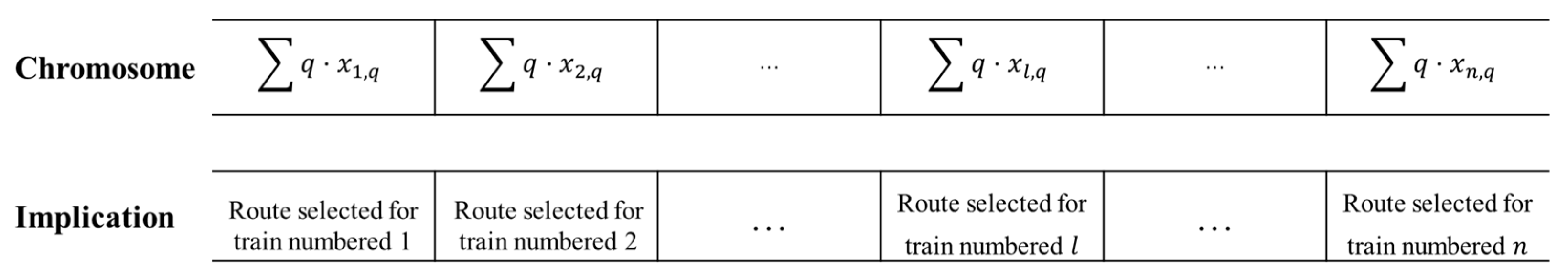
4.1. Rules of Chromosome Encoding and Decoding
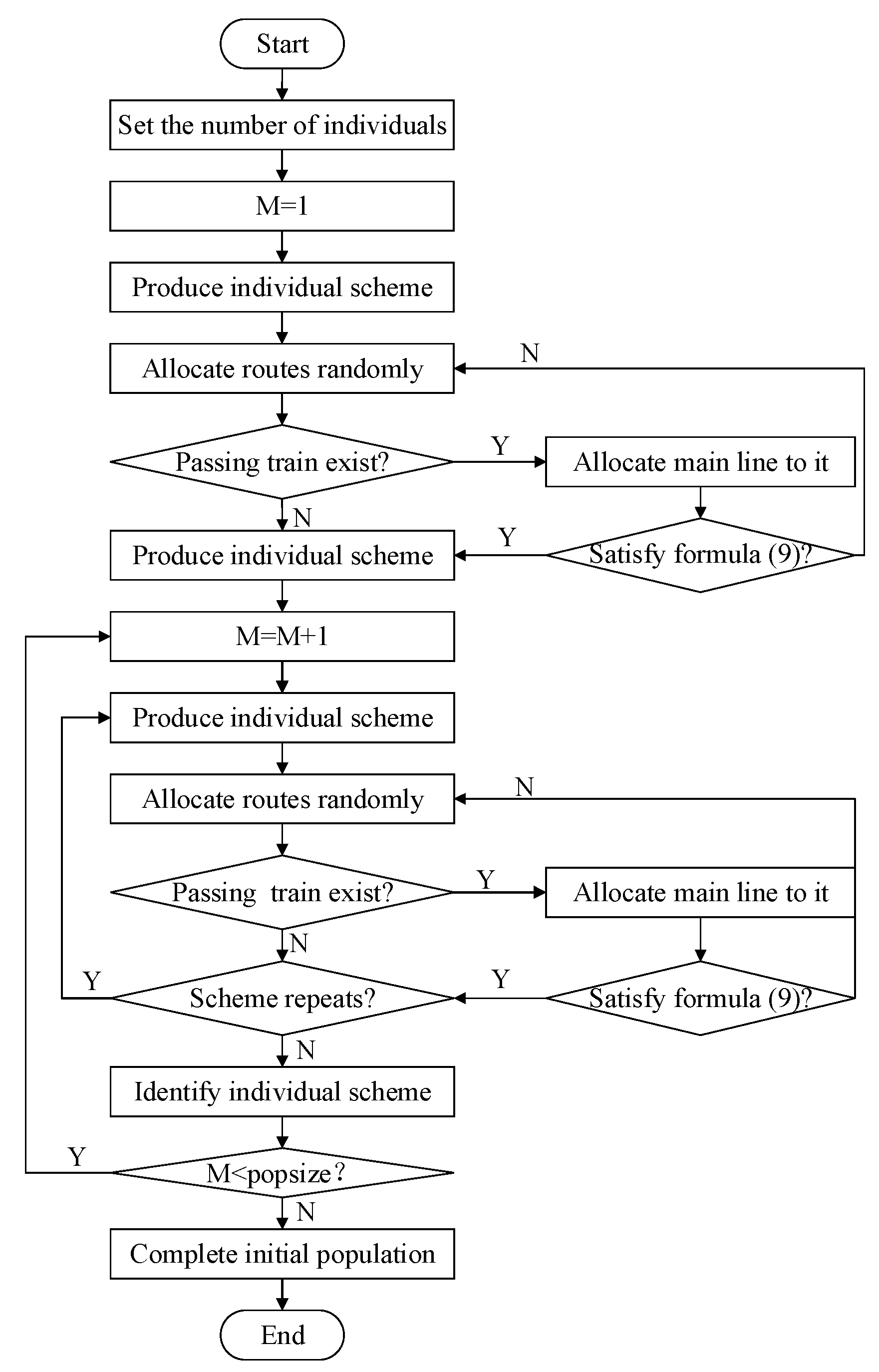
4.2. Generation of an Initial Population
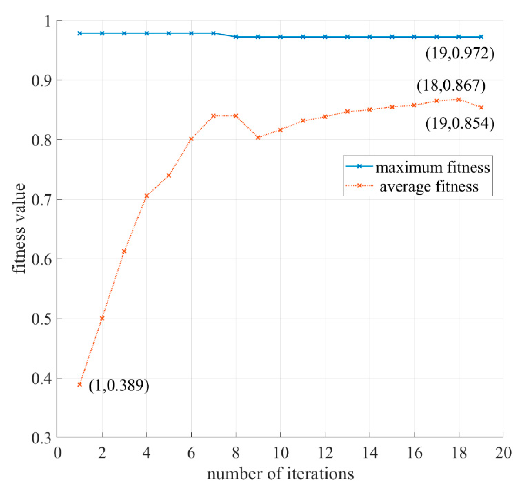
4.3. Fitness Function Setting
4.4. Algorithm Termination Condition
4.5. Genetic Operators with Elitist and Adaptive Strategies
- Calculate the number of chromosomes for crossover as ( is the total number of individuals in a generation).
- Compare a randomly generated number between 0 and 1 with . If is greater and the genotypes of adjacent chromosomes are different, perform crossover.
- Generate a random number ().
- Exchange all genes after gene point to obtain two new progenies from two adjacent chromosomes.
- Check if the constraints on the individuals after crossover are met. If yes, the crossover operation is completed. Otherwise, repeat the second step.
5. Case Study
5.1. Station Background Setting
5.2. Scenario Setting and Operation Process
5.3. Performance Analysis of Multiple Operations
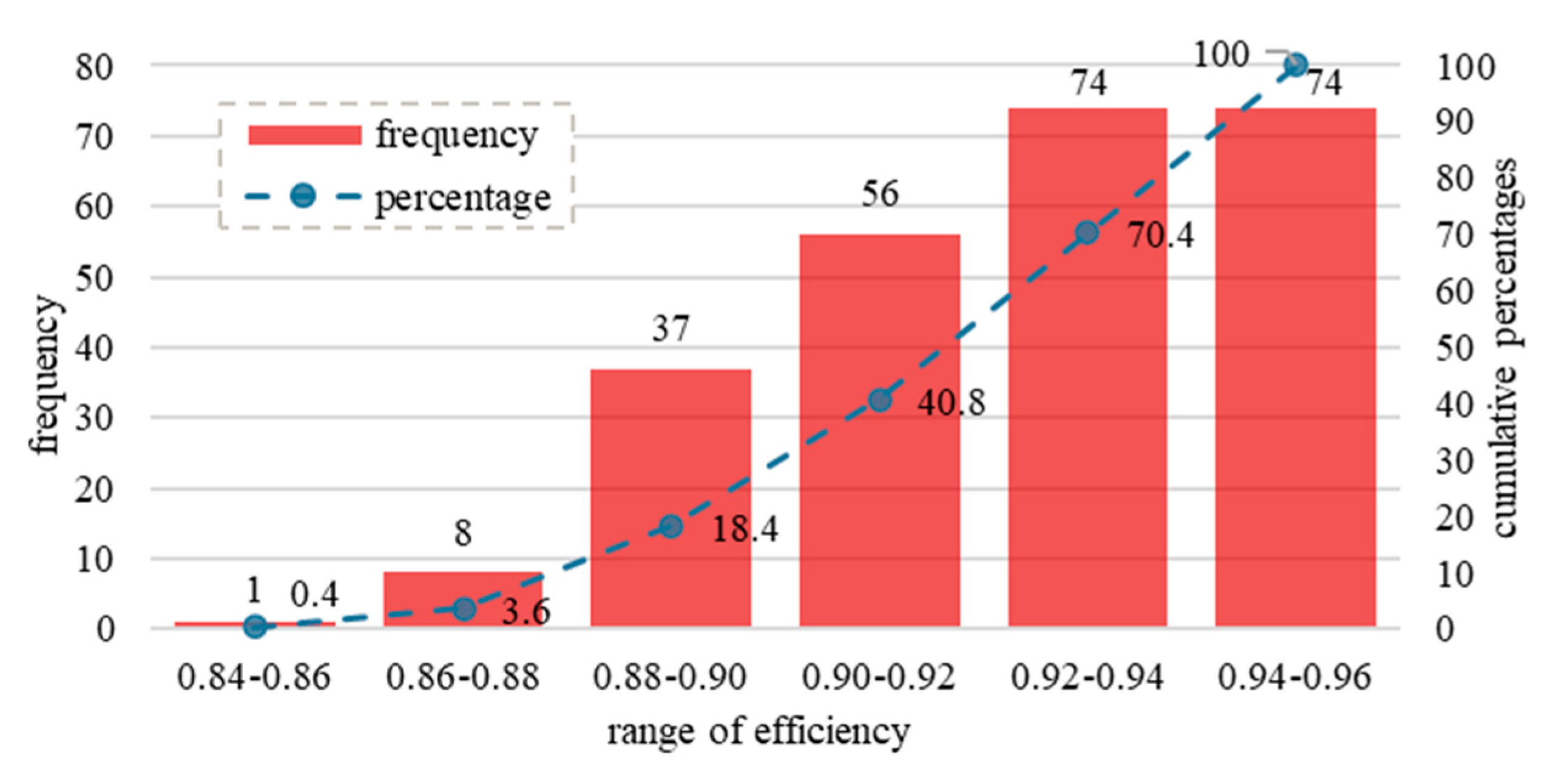
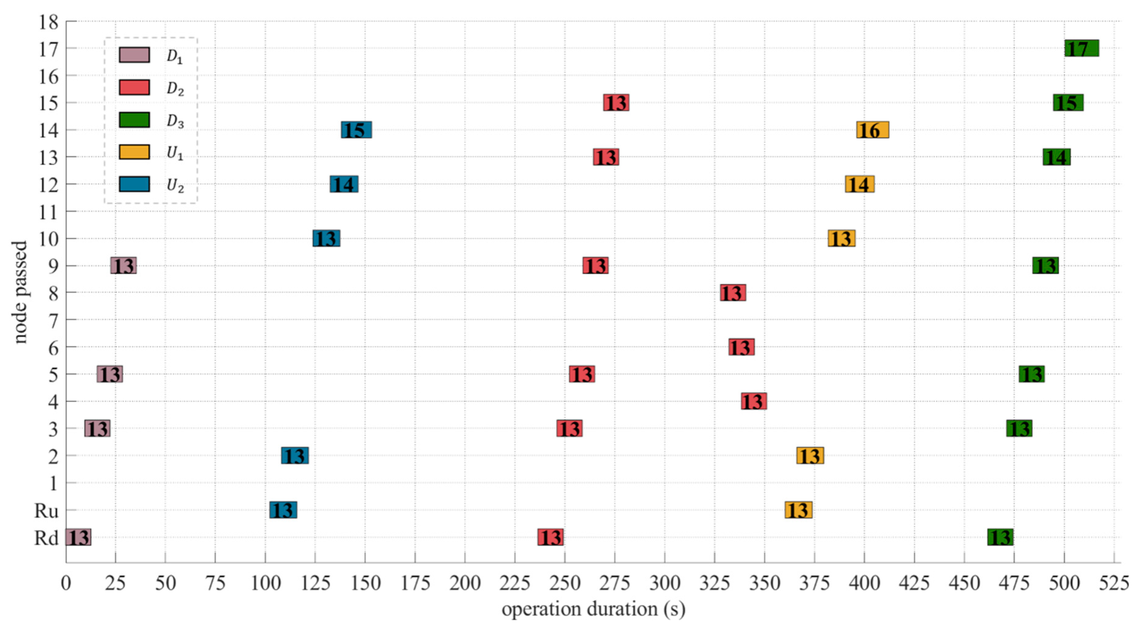
5.4. Results Analysis for Obtaining an Individual Scenario
6. Discussion, Conclusions, and Future Research
Author Contributions
Funding
Data Availability Statement
Conflicts of Interest
References
- Bock, U.; Bikker, G. Design and Development of a Future Freight Train Concept—Virtually Coupled Train Formation. IFAC Proc. 2000, 33, 395–400. [Google Scholar] [CrossRef]
- Bock, U.; Varchmin, J.U. Virtually coupled train formations: Wireless communication between train units. In Proceedings of the General Traffic Forum 2000, Braunschweig, Germany, 6–7 April 2000; pp. 165–174. [Google Scholar]
- Songnian, Z.; Rui, S. Theoretical Analysis on Combinatorial Control of the Trains Velocities System. J. China Railw. Soc. 1997, 19, 10–16. [Google Scholar]
- Ning, B. Absolute braking and relative distance braking—Train operation control modes in moving block systems. Trans. Built Environ. 1998, 34, 991–1001. [Google Scholar]
- European Union. Council Regulation (EU) No 642/2014 of 16 June 2014 Establishing the Shift2Rail Joint Undertaking. Available online: https://eur-lex.europa.eu/eli/reg/2014/642/oj (accessed on 17 June 2014).
- Construcción y Auxiliar de Ferrocarriles. Connected Trams Demonstrator Brochure. Available online: https://projects.shift2rail.org/s2r_ip1_n.aspx?p=CONNECTA (accessed on 30 August 2018).
- Aljama, P. Applicability of 5G Technology for a Wireless Train Backbone. In Proceedings of the 15th European Conference on Antennas and Propagation, Dusseldorf, Germany, 22–26 March 2021; pp. 1–5. [Google Scholar]
- Shift2Rail. Virtual Train Coupling System Concept and Application Conditions. Available online: https://projects.shift2rail.org/s2r_ip_TD_D.aspx?ip=2&td=aa1f0995-1402-4e7b-a905-49fba1bc6f71 (accessed on 15 January 2020).
- Shift2Rail. Market Potential and Operational Scenarios for Virtual Coupling. Available online: https://projects.shift2rail.org/s2r_ip_TD_D.aspx?ip=2&td=aa1f0995-1402-4e7b-a905-49fba1bc6f71 (accessed on 19 July 2019).
- Shift2Rail. Application Roadmap for the Introduction of Virtual Coupling. Available online: https://shift2rail.org/news/results-published-in-february (accessed on 25 February 2021).
- Shift2Rail. Business Risk Analysis of Virtual Coupling. Available online: https://shift2rail.org/news/results-published-in-january/ (accessed on 2 December 2020).
- Stickel, S.; Schenker, M.; Dittus, H.; Unterhuber, P.; Canesi, S.; Riquier, V.; Ayuso, E.P.; Berbineau, M.; Goikoetxea, J. Technical feasibility analysis and introduction strategy of the virtually coupled train set concept. Sci. Rep. 2022, 12, 4248. [Google Scholar] [CrossRef] [PubMed]
- Bingxun, L.; Chengyun, C.; Xianying, C. Skip and Stop Scheduling based on Virtually Coupled Trains. J. Korean Soc. Railw. 2020, 23, 80–88. [Google Scholar]
- Shican, W.; Xianying, C. Protection Algorithm for Virtual Coupler in T2T-Based Autonomous Train Control System. J. Korean Inst. Commun. Inf. Sci. 2018, 43, 1894–1902. [Google Scholar]
- Junfeng, C. Discussion on Development of Future Rail Transit Train Control System. Railw. Signal. Commun. Eng. 2020, 17, 1–4. [Google Scholar]
- Junfeng, C.; Ling, L. Research on Key Technology Requirements of Virtual Coupling in Application of Train Control System. Railw. Signal. Commun. Eng. 2019, 16, 1–5. [Google Scholar]
- Xinde, M.; Jianming, Z. A Rescue Method under Virtually-Coupled Train Sets Based on Active Recognition. CN108216302B, 14 February 2020. [Google Scholar]
- Yong, Z.; Haifeng, W. Topological manifold-based monitoring method for train-centric virtual coupling control systems. IET Intell. Transp. Syst. 2020, 14, 91–102. [Google Scholar]
- Xue, L.; Caiqing, M.; Qianling, W. Dual Jitter Suppression Mechanism-Based Cooperation Control for Multiple High-Speed Trains with Parametric Uncertainty. Mathematics 2023, 11, 1786. [Google Scholar]
- Yuan, C.; Jiakun, W.; Lianchuan, M. Dynamic marshalling and scheduling of trains in major epidemics. J. Traffic Transp. Eng. 2020, 20, 120–128. [Google Scholar]
- Quaglietta, E. Analysis of platooning train operations under v2v communication-based signaling: Fundamental modelling and capacity impacts of virtual coupling. In Proceedings of the 98th Transportation Research Board Annual Meeting, Washington, DC, USA, 13–17 January 2019; pp. 19–01043. [Google Scholar]
- Quaglietta, E. Intelligent Dispatching and Coordinated Control Method at Railway Stations for Virtually Coupled Train Sets. J. Rail Transp. Plan. Manag. 2020, 3, 100237. [Google Scholar]
- Ling, L.; Peng, W. A multi-state train-following model for the analysis of virtual coupling railway operations. In Proceedings of the 2019 IEEE Intelligent Transportation Systems Conference, Auckland, New Zealand, 27–30 October 2019; pp. 607–612. [Google Scholar]
- Liu, L.; Wang, P.; Wang, Y. Dynamic train formation and dispatching for rail transit based on virtually coupled train set. In Proceedings of the 2019 IEEE Intelligent Transportation Systems Conference, Auckland, New Zealand, 27–30 October 2019; pp. 2823–2828. [Google Scholar]
- Schuman, T. Increase of capacity on the Shinkansen high-speed line using virtual coupling. Int. J. Transp. Dev. Integr. 2014, 1, 666–676. [Google Scholar] [CrossRef]
- Xun, J.; Chen, M.; Ning, B.; Tang, T.; Dong, H. Train tracking performance measurement under virtual coupling in subway. J. Beijing Jiaotong Univ. 2019, 43, 91–102. [Google Scholar]
- Zhou, X.; Fang, L.; Liyu, W. Optimization of Train Operation Planning with Full-Length and Short-Turn Routes of Virtual Coupling Trains. Appl. Sci. 2022, 12, 7935. [Google Scholar] [CrossRef]
- Janusz, S.; Kochan, A. Maximization of Energy Efficiency by Synchronizing the Speed of Trains on a Moving Block System. Energies 2023, 16, 1764. [Google Scholar]
- Xu, Y.; Cao, C.X.; Li, M.H.; Luo, J.L. Modeling and Simulation for Urban Rail Traffic Problem Based on Cellular Automata. Commun. Theor. Phys. 2012, 58, 847–855. [Google Scholar] [CrossRef]
- Ning, B.; Dong, H.; Gao, S.; Tang, T.; Zheng, W. Distributed cooperative control of multiple high-speed trains under a moving block system by nonlinear mapping-based feedback. Sci. China Inf. Sci. 2018, 61, 120202. [Google Scholar] [CrossRef]
- Zhou, H.; Zhou, L.; Guo, B.; Bai, Z.; Wang, Z.; Yang, L. A Scheduling Approach for the Combination Scheme and Train Timetable of a Heavy-Haul Railway. Mathematics 2021, 9, 3068. [Google Scholar] [CrossRef]
- Lin, F.; Liu, S.; Yang, Z.; Zhao, Y.; Yang, Z.; Sun, H. Multi-Train Energy Saving for Maximum Usage of Regenerative Energy by Dwell Time Optimization in Urban Rail Transit Using Genetic Algorithm. Energies 2016, 9, 208. [Google Scholar] [CrossRef]
- Liu, Y.; Liu, R.; Wei, C.; Xun, J.; Tang, T. Distributed Model Predictive Control Strategy for Constrained High-Speed Virtually Coupled Train Set. IEEE Trans. Veh. Technol. 2022, 71, 171–183. [Google Scholar] [CrossRef]
- Ming, C.; Haoxiang, S.; Hongjie, L. Long Short-Term Memory-Based Model Predictive Control for Virtual Coupling in Railways. Wirel. Commun. Mob. Comput. 2022, 2022, 1859709. [Google Scholar]
- Felez, J.; Vaquero-Serrano, M.A.; de Dios Sanz, J. A Robust Model Predictive Control for Virtual Coupling in Train Sets. Actuators 2022, 11, 372. [Google Scholar] [CrossRef]
- Yijuan, H.; Jidong l Hongjie, L.; Tang, T. Toward the Trajectory Predictor for Automatic Train Operation System Using CNN–LSTM Network. Actuators 2022, 11, 247. [Google Scholar]
- Li, S.E.; Zheng, Y.; Li, K.; Wang, L.Y.; Zhang, H. Platoon Control of connected Vehicles from a Networked Control Perspective: Literature Review, Component Modeling, and Controller Synthesis. IEEE Trans. Veh. Technol. 2017. [Google Scholar] [CrossRef]
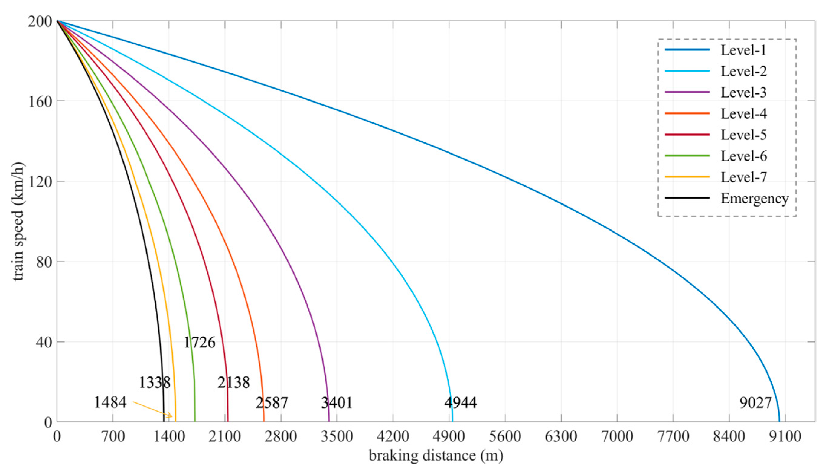
- Wenliang, Z.; Yinling, W. Braking Calculation of Electric Multiple Units. J. Tongji Univ. 2017, 45, 119–123. [Google Scholar]
- GB/T 25338.1-2019; Switch Machines for Railways—Part 1: General Specification China. National Railway Administration of the People’s Republic of China: Xi’an, China, 2019.
- ISO 2631-5:2018; Mechanical Vibration and Shock—Evaluation of Human Exposure to Whole-Body Vibration—Part 5: Method for Evaluation of Vibration Containing Multiple Shocks. ISO: Geneva, Switzerland, 2018.


| Index | Performance |
|---|---|
| Allowable lateral through speed (km/h) | 80 |
| Allowable straight through speed (km/h) | 350 |
| Total length of turnout (mm) | 6900 |
| Distance between tracks (mm) | 4600 |
| Conversion duration (s) | 13 |
| Operating Capacity or Working Habit | Number of Station Line | ||||||
|---|---|---|---|---|---|---|---|
| Ⅰ | Ⅱ | 3 | 4 | 5 | 6 | 7 | |
| Train passing through | 1 | 1 | 0.05 | 0.05 | 0.05 | 0.05 | 0.05 |
| Train reception on up direction | 0.1 | 0.5 | 0.7 | 1 | 0.7 | 1 | 0.6 |
| Train reception on down direction | 0.5 | 0.1 | 1 | 0.7 | 1 | 0.7 | 1 |
| Train departure on up direction | 0.1 | 0.5 | 0.7 | 1 | 0.7 | 1 | 0.6 |
| Train departure on down direction | 0.5 | 0.1 | 1 | 0. 7 | 1 | 0.7 | 1 |
| Shutting in and out of the depot | 0.8 | 0.8 | 1 | 0.6 | 1 | 0.6 | 0.9 |
| Serving and technical inspection | 0.5 | 0.5 | 0.8 | 0.8 | 0.9 | 0.9 | 1 |
| Passenger alighting and boarding | 0.2 | 0.2 | 1 | 1 | 1 | 1 | 1 |
| Passengers’ walking distance | 0.1 | 0.1 | 0.9 | 0.8 | 1 | 0.7 | 1 |
| Degree | |||||
|---|---|---|---|---|---|
| 0–5 | 5–20 | 20–70 | 70–118 | 118–200 | |
| Level-2 | 0.2470 | 0.2180 + 0.0057956 | 0.3339 | 0.3694 − 0.0005066 | 0.3847 − 0.000637 |
| Emergency | 0.9990 | 0.8820 + 0.0234000 | 1.3500 | 1.3879 − 0.0005418 | 1.8752 − 0.004672 |
| Index | VCTS from Down Direction | VCTS from Up Direction |
|---|---|---|
| Number of EMUs | ||
| Full length (m) | 211 | 211 |
| Approach speed (km/h) | 80 | 75 |
| Train interval (m) | 900 | 850 |
| Braking model | Level-2 | Level-2 |
| Operating Requirement | Number of Trains | ||||
|---|---|---|---|---|---|
| Train passing through | 0 | 1 | 0 | 0 | 0 |
| Train reception on up direction | 0 | 0 | 0 | 1 | 1 |
| Train reception on down direction | 1 | 0 | 1 | 0 | 0 |
| Train departure on up direction | 0 | 0 | 0 | 0 | 0 |
| Train departure on down direction | 0 | 0 | 0 | 0 | 0 |
| Shutting in and out of the depot | 0 | 0 | 0 | 1 | 0 |
| Serving and technical inspection | 0.9 | 0 | 0.8 | 0 | 0.6 |
| Passengers’ alighting and boarding | 0.9 | 0 | 0 | 1 | 0.9 |
| Passengers’ walking distance | 0.8 | 0 | 0 | 0.9 | 0.3 |
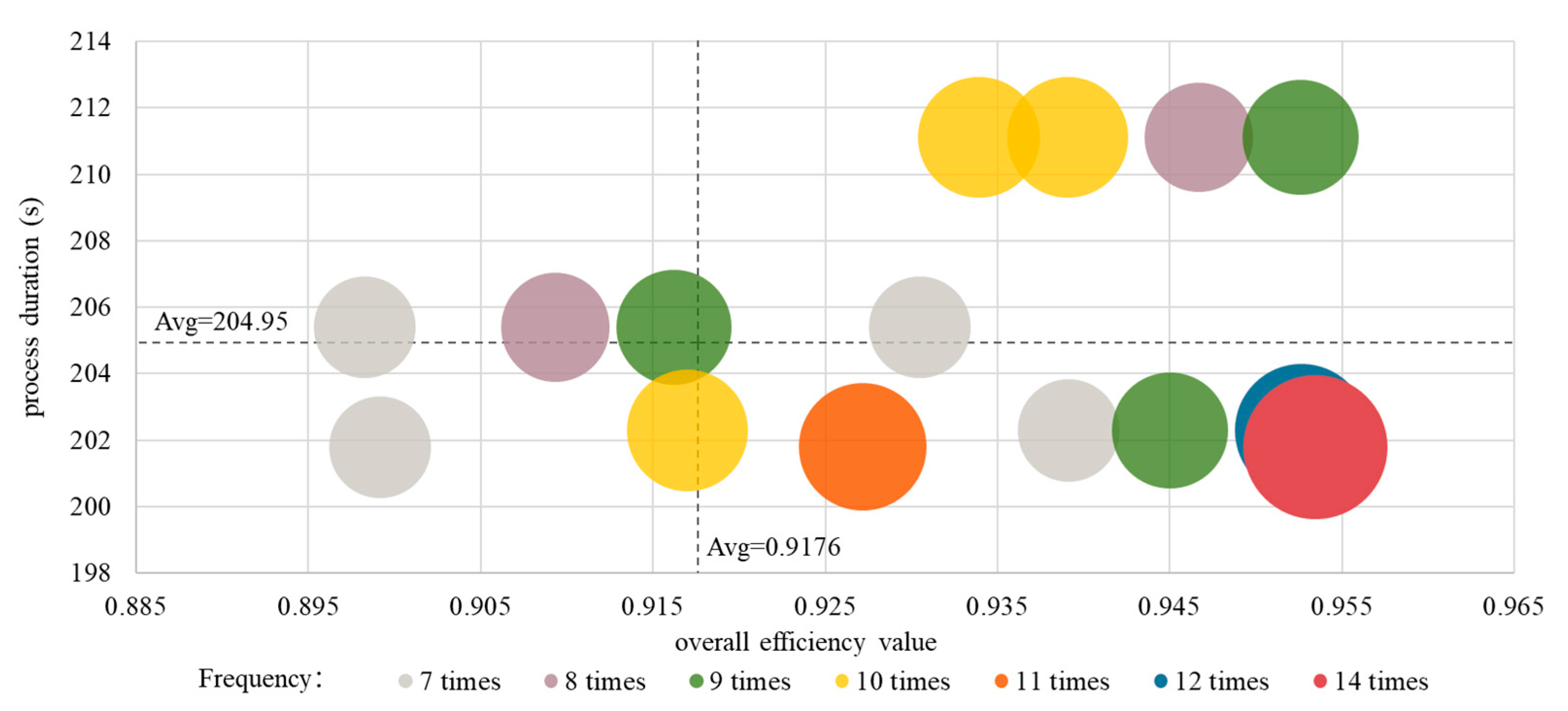
| Index | Value | ||||
|---|---|---|---|---|---|
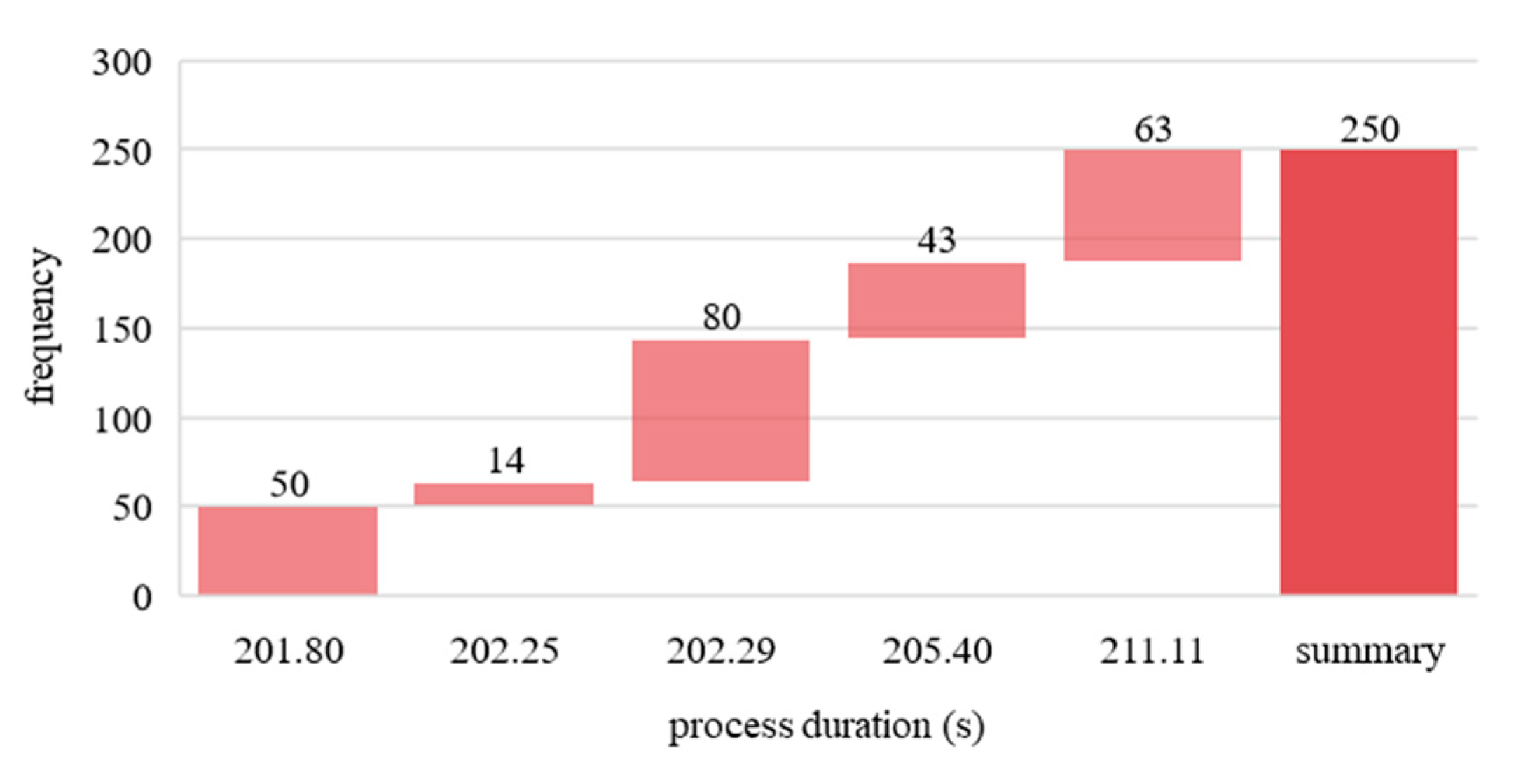
| Process duration (s) | 201.80 | 202.25 | 202.29 | 205.40 | 211.11 |
| 5 | 6 | 7 | 4 | 3 | |
| 0.9556 | 0.7889 | 1 | 0.7444 | 0.9111 | |
| Frequency | 50 | 14 | 80 | 43 | 63 |
| Cumulative percent (%) | 20.0 | 5.6 | 32.0 | 17.2 | 25.2 |
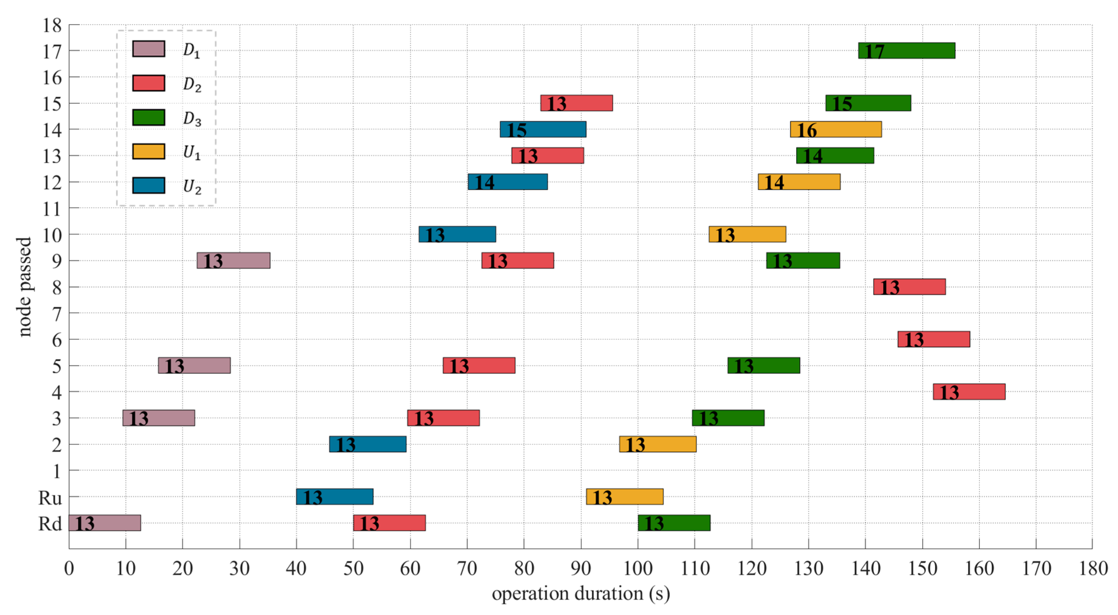
| EMUs | Selected Track | Operation Duration (s) | Timing Range (s) | Effectiveness (%) |
|---|---|---|---|---|
| 7 | 102.21 | 0–102.21 | 100.00 | |
| I | 123.80 | 50.04–173.84 | 100.00 | |
| 5 | 101.72 | 100.08–201.80 | 95.56 | |
| 4 | 104.17 | 40.00–144.17 | 85.13 | |
| 6 | 101.39 | 90.98–192.36 | 94.64 | |
| Overall | 533.29 | 201.80 | 92.55 | |
| EMUs | Index | Nodes | |||||||||||
|---|---|---|---|---|---|---|---|---|---|---|---|---|---|
| 1 | 3 | 5 | 7 | 9 | 11 | 13 | 15 | 17 | Stop | ||||
| ST | 0.00 | — | 9.50 | 15.75 | — | 22.55 | — | — | — | — | 102.21 | — | |
| FT | 12.65 | — | 22.14 | 28.40 | — | 35.37 | — | — | — | — | — | — | |
| IS | 80.00 | — | 80.00 | 80.00 | — | 80.00 | — | — | — | — | 0.00 | — | |
| ST | 50.04 | — | 59.54 | 65.79 | — | 72.59 | — | 77.85 | 82.94 | — | 131.54 | 161.19 | |
| FT | 62.69 | — | 72.18 | 78.44 | — | 85.23 | — | 90.50 | 95.58 | — | 144.18 | 173.84 | |
| IS | 80.00 | — | 80.00 | 80.00 | — | 80.00 | — | 80.00 | 80.00 | — | 80.00 | 80.00 | |
| ST | 100.08 | — | 109.58 | 115.83 | — | 122.63 | — | 127.89 | 133.04 | 138.79 | 201.80 | — | |
| FT | 112.73 | — | 122.22 | 128.48 | — | 135.49 | — | 141.49 | 147.98 | 155.76 | — | — | |
| IS | 80.00 | — | 80.00 | 80.00 | — | 80.00 | — | 80.00 | 76.43 | 69.63 | 0.00 | — | |
| EMUs | Index | Nodes | |||||||||
|---|---|---|---|---|---|---|---|---|---|---|---|
| 2 | 4 | 6 | 8 | 10 | 12 | 14 | Stop | ||||
| ST | 40.00 | 45.81 | — | — | — | 61.55 | 70.19 | 75.81 | 144.17 | — | |
| FT | 53.49 | 59.30 | — | — | — | 75.04 | 84.13 | 90.91 | — | — | |
| IS | 75.00 | 75.00 | — | — | — | 75.00 | 75.00 | 75.00 | — | — | |
| ST | — | — | 151.92 | 145.71 | 141.44 | — | — | — | — | — | |
| FT | — | — | 164.57 | 158.36 | 154.08 | — | — | — | — | — | |
| IS | — | — | 80.00 | 80.00 | 80.00 | — | — | — | — | — | |
| ST | 90.98 | 96.78 | — | — | — | 112.53 | 121.17 | 126.82 | 192.36 | — | |
| FT | 104.46 | 110.27 | — | — | — | 126.03 | 135.58 | 142.84 | — | — | |
| IS | 75.00 | 75.00 | — | — | — | 75.00 | 75.00 | 72.64 | — | — | |
Disclaimer/Publisher’s Note: The statements, opinions and data contained in all publications are solely those of the individual author(s) and contributor(s) and not of MDPI and/or the editor(s). MDPI and/or the editor(s) disclaim responsibility for any injury to people or property resulting from any ideas, methods, instructions or products referred to in the content. |
© 2023 by the authors. Licensee MDPI, Basel, Switzerland. This article is an open access article distributed under the terms and conditions of the Creative Commons Attribution (CC BY) license (https://creativecommons.org/licenses/by/4.0/).
Share and Cite
Zhang, Y.; Xu, Q.; Yu, R.; Zhao, M.; Liu, J. Receiving Routing Approach for Virtually Coupled Train Sets at a Railway Station. Mathematics 2023, 11, 2002. https://doi.org/10.3390/math11092002
Zhang Y, Xu Q, Yu R, Zhao M, Liu J. Receiving Routing Approach for Virtually Coupled Train Sets at a Railway Station. Mathematics. 2023; 11(9):2002. https://doi.org/10.3390/math11092002
Chicago/Turabian StyleZhang, Yinggui, Qianying Xu, Runchuan Yu, Minghui Zhao, and Jiachen Liu. 2023. "Receiving Routing Approach for Virtually Coupled Train Sets at a Railway Station" Mathematics 11, no. 9: 2002. https://doi.org/10.3390/math11092002