Abstract
There are few examples of mechanical coupling solutions for the transmission of high torques between two rotating shafts that have non-coplanar, non-parallel axes. Based on the structural analysis, the paper proposes a solution for an RP1PR-type symmetrical coupling. The Hartenberg–Denavit methodology is not applicable for performing the kinematical analysis, hence the solution starts from the geometrical condition of the creation of planar pairs of the mechanism, expressed in vector form. The absolute motion of all elements of the mechanism’s structure can be expressed after developing the kinematical analysis. The theoretical results are validated via numerical analysis. By comparing the analytical results with the CATIA-modeled results, excellent compatibility is obtained. We also propose a constructive solution for the newly designed coupling mechanism.
Keywords:
spatial coupling; crossed axes; kinematic analysis; constructive solutions; numerical validation MSC:
70B15; 70B10; 00A06; 65D17
1. Introduction
One of the main tasks of the Theory of Machines and Mechanisms is the transmission of rotational motion between two fixed axes. The problem arose even from the first machines, which had complex requirements while the driving possibilities were limited, as is still the case [1,2]. A mobile assembly is actuated for most cases by rotational engines—cc, dc, or internal combustion engine—when the driving element has a rotational motion, and by free piston linear engine when a translational motion is needed. Obviously, the motion of the final element depends on the construction of the kinematical chain interposed between the driving and driven elements. The designer is responsible for choosing amongst possible solutions the one that best runs the transmission [3]. From these criteria, one can mention a kinematical criterion [4,5], which imposes a certain law of motion for the driven element, constructive simplicity [6,7,8], high efficiency, low production costs, high accuracy [9,10], etc. However, the higher the number of imposed criteria, the fewer possibilities of completely fulfilling them. Therefore, a prioritization of criteria is necessary for choosing the final solution [11]. The solution can either be adapted to the actual necessities, or a completely new one must be found. The latter case requires comprehensive study and research work since a new solution should be original and comparable or superior to the existing ones from the point of view of fulfilling the imposed criteria.
The present paper proposes a new coupling mechanism with high reliability and an original method for the kinematical analysis, based on a geometrical condition concerning the creation of planar pairs.
The kinematics analysis of a spatial mechanism can be completed by the general methodology proposed by Hartenberg and Denavit [12], known as the “the method of homogenous operators”, which is appropriate for spatial bar mechanisms having in their structure only cylindrical pairs, or particular cases of cylindrical pairs: revolute pair, prismatic pair, or helical pair [13]. The method is based on the relations of transformation of a point’s coordinates when the reference system is changed and expresses the condition of closure of the mechanism’s kinematic chain in matrix form—using square type 4 × 4 matrices. For the situations when other than cylindrical pairs occur in the structure of the mechanisms, the method proposed by Hartenberg and Denavit can be applied after each of the non-cylindrical joints is replaced by a kinematical chain that has in its structure only cylindrical pairs [14,15].
Fisher presents solutions for substituting the spherical joints by an assembly of three revolute pairs with concurrent and reciprocally perpendicular axes [16]. Fisher also proposes the replacement of a planar joint by an assembly of two prismatic joints with perpendicular axes and a revolute joint with the axis normal to the plane defined by the revolute pairs. In [17] there is presented a methodology of replacing a class 1 pair with a mechanism consisting of two shafts with direct contact and crossed directions. Generally, when applying the Hartenberg and Denavit method, this produces complicated systems of trigonometrical equations that can rarely be solved analytically. One of the difficulties met in the positional solutioning of a spatial mechanism is the fact that the system of trigonometrical equations obtained presents multiple solutions—solutions corresponding to all assembling possibilities of the mechanism when the values of the driving element’s position parameters are stipulated.
Another aspect that complicates solving the positional analysis of a spatial mechanism is the structure of a homogenous operator’s matrix. This matrix has a structure that contains the rotational matrix, which describes the position of the new system of coordinates with respect to the initial one, and the displacement vector corresponding to the translation of the old origin into the new position. Two displacements are identical when the matrices corresponding to the homogenous operators correlated to the two displacements are identical [12]. The identification of the elements of displacement vectors produces three scalar equations and the identification of the rotation matrices gives nine scalar equations from which only three are independent. These three independent equations are recognized by deconstructing the rotation matrix into symmetric and antisymmetric matrices [18], followed by finding the versor of the rotation axis and the rotation angle. At this stage the conditions of equality of rotations can be imposed, specifically the axis parallelism, resulting in two scalar equations, and the equality of the rotation angles, which results in the third scalar equation.
Lastly, six scalar trigonometrical equations result from the condition that two displacements are identical. From here, the conclusion is that the simplest spatial mechanism with mobility , which has the kinematic completely determined by the conditions developed from the contour closure condition, has the position described by six scalar parameters. Uicker et al. [19] developed a numerical methodology that considers a constrained system of 12 scalar equations obtained by equalling all components of the displacement vectors and rotation matrices. The procedure is iterative, rapidly converging, and finally offering the position parameters of the mechanism of single-contour mechanism. The fact that the numerical methodology is appropriate to an over-constrained system of equations leads to the idea of applying it to over-constrained mechanisms. In the literature, there are presented the kinematical solutions for the Bricard mechanism [12,20], and Benett mechanism [12]. In the case where the mechanism contains numerous contours whose positions cannot be described by six scalar parameters, the equations resulting from the closing matrix equations of some loops will be considered until the number of obtained scalar equations will equal the number of scalar parameters of position of all the considered kinematical chains.
There are numerous types of couplings in technical applications [1,14,21,22,23,24,25], but the couplings with crossed axes of high reliability and that transmit important torques are rather infrequent. The present paper proposes a new coupling mechanism of an RP1PR type, an original method for the kinematics analysis, and the design of the corresponding constructive solution.
2. Structural Considerations
Figure 1 shows two shafts with crossed axes and the coupling intermediate kinematic chain consisting of elements and kinematic pairs of class k. The two shafts are joined to the ground by revolute pairs . The transmission has a unique driving element, 1 and that means that the mobility of the transmission should be . The formula for the calculus of the mobility degree of spatial mechanisms [21] is:
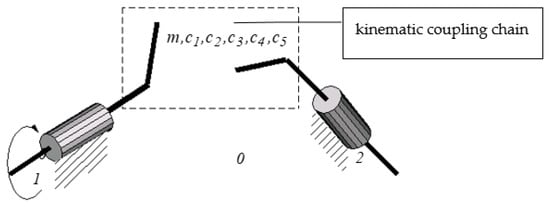
Figure 1.
Transmission of rotation motion between two shafts with crossed axes through an intermediate chain.
Applying the relation (1) for the particular case from Figure 1 gives:
where represents the number of degrees of freedom nulled by the coupling kinematic chain composed of m elements.
The final relation is:
Equation (3) allows for finding the number of elements and kinematic joints from the structure of the coupling chain. The simplest coupling solution corresponds to , that is direct coupling of the two shafts. For Equation (3) has one solution:
which shows that between the two shafts a pair of class (direct point contact) must exist. The concrete form can be the contact between two surfaces (gear mechanisms with crossed axes [26,27] or spatial cam mechanisms [28]), two curves [29], the contact between a surface and a point, point-curve contact, or curve-surface contact [30]. The above enumeration demonstrates that even for the simplest case of direct transmission, the constructive solutions are numerous. The advantage of this structural solution is its constructive simplicity. While the main drawback can be considered to be the high contact stresses from the contact pair between the two elements [31,32,33,34]. The next structural solution, , with a single intermediate element, gives the relation:
There are multiple structural solutions since the kinematic coupling chain can contain any type of kinematic pair. In [35] it is presented the constructive solution:
Next, a new solution is presented, where the coupling consists of revolute–planar–contact–planar–revolute (acronym RP1PR) joints. Possible pairs that can be used in the structure of the mechanism are:
- another class 3 pair could be the spherical joint, Figure 3a.

Figure 3.
Constructive solution for spherical pairs: (a) spherical pair; (b) spherical pair with pin.
Figure 3.
Constructive solution for spherical pairs: (a) spherical pair; (b) spherical pair with pin.

Therefore, an alternate mechanism (to our proposed RP1PR) is RS1SR, that is, to use spherical joints (Figure 3a). In this case, the first significant problem that arises concerns a passive motion of the intermediate element about the axis passing through the centers of spheres. To eliminate this passive motion, one of the spherical joints must be replaced by a joint of finger-sphere type of class 4 (Figure 3b). From the figures representing the planar and spherical joints, it is obvious that the class 3, planar joint is preferable. In the case of a spherical pair, the constructive solution is more complex from a manufacturing point of view [36,37] because the planar pair consists of plane surfaces obtained by high machining conditions, compared to the spherical surfaces, (especially inner spherical surfaces) which are difficult to obtain technologically.
From a functional perspective, the planar pair is also desirable because it presents the advantage that the three allowed motions (two translations and one rotation) are not limited, while, for the spherical joint, (three rotations allowed) there are imposed some constructive restrictions and locking of the mechanism may occur.
2.1. Proposed Solution
One of the possible solutions that verify the relation (5) corresponds to the case when the intermediate element makes with the rest of the elements two planar pairs of class 3 and a pair of class 1 (RP1PR). The principle scheme for designing the mechanism is presented in Figure 4a, and the kinematic diagram of the mechanism is shown in Figure 4b. The middle element consists of the planes and fixed together, having a dihedral angle of and B the point from the intersection line. Driving shaft 1 and driven shaft 2 have the planes and attached respectively and is the plane fixed to the ground. The mechanism is created when the coincidence between the planes − , and respectively is ensured and the point B is obliged to lay in the plane .
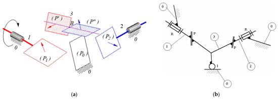
Figure 4.
Proposed mechanism (0—the ground; 1—the driving element; 2—the driven element; 3—the middle element): (a) principle schematics for designing the mechanism; (b) kinematic diagram.
The elements of the mechanism are shown in Figure 4b, represented according to international standards [38]: the ground 0, the driving element 1, the driven (exit) element 2, and the intermediate element 3. The joints of the mechanism are: two revolute pairs R (first, between the ground and the driving element and the second, between the driven element and the ground), two planar pairs P (between the driving element and the intermediate element and, between the intermediate element and the driven element, respectively), and 1, a class 1 pair (point contact between the middle element and the ground). The succession of the pairs is the origin of the abbreviation of the name of the mechanism: RP1PR. We must mention that in the literature [1,39], only nine possible structural solutions for spatial mechanisms with intermediate elements are presented. The proposed RP1PR coupling is an entirely new solution.
The kinematic analysis of the mechanism requires finding the motion from the pairs of the mechanism. A convenient method consists in equivalating the planar joints with an assembly of two prismatic pairs with perpendicular axes and a revolute pair with the axis normal to the prismatic pairs and then replacing the class 1 pair with a series Oldham coupling–Cardan coupling [21]. The Hartenberg–Denavit method could be applied to the obtained mechanism. The disadvantage of the kinematic solution resides in a great number of elements and kinematic pairs of the substituting mechanism.
The graph of the mechanism is presented in Figure 5 and it contains two independent contours: and . The position of the first contour is defined by scalar parameters and the position of the second is described by scalar parameters.

Figure 5.
The graph of the mechanism.
Thus, we conclude that neither of the two contours can be analyzed independently, through the six scalar equations obtained from the condition of the closed kinematic chain. Instead, considering the two contours simultaneously, for obtaining the complete stipulation of the positions, there are required scalar parameters that can be unequivocally found from the 12 scalar equations of closure of the two loops. As mentioned above, solving the system of 12 trigonometrical equations will encounter difficulties. Therefore, a method where the conditions of forming the joints of the mechanism are directly used is preferred to the classical Hartenberg–Denavit method.
Several coordinate systems are used for solving the problem, as shown in Figure 6. The coordinate system of the ground, with the axis as common normal for the axes of the two shafts. The origin of the fixed system is in the middle of the common normal . The axes of the two shafts make two planes with the common normal, and their bisecting plane is . The distance between the axes of the shafts is and the angle between them is . The axis is in completion for the tri-orthogonal right reference system.
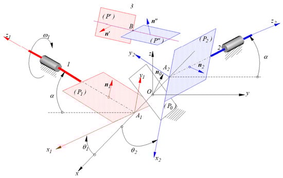
Figure 6.
The coordinate systems and the kinematic and constructive parameters of the mechanism.
To each of the two shafts, a mobile coordinate system is attached, with the axis in coincidence with the axis of the shaft, with the origin in the foot of the common normal. The plane is the plane with the normal that contains the point and the plane is the plane with the normal that contains the point The plane , of normal in which the point is obliged to move, is considered to be a plane containing the common normal of the axes and of the two shafts, and making the angle with the axis . This position was chosen in order to obtain simpler relations. Obviously, a generic position can be chosen for the plane and the methodology for finding the solution is the same, but only with increased amounts of calculus. The positions of the two shafts will be stipulated by the angles and made by the axes and with the axis.
The creation of planar joints imposes the next geometrical conditions:
- the planes and should be perpendicular:
- the point belongs to the plane :
- the point belongs to the plane :
The creation of the contact between the sphere and the plane requires:
- the point belongs to the plane :
For the proposed RP1PR mechanism, the relations (7)–(10) are needed and all vectors must be expressed in the same frame. The coordinate system of the ground is chosen for this purpose. The notation will be subsequently used to specify the coordinate system, other than the fixed one, where the Cartesian components of the vector are stipulated. For a simplified notation, the lack of exponent indicates that the vector is outlined by the Cartesian projections on the axes of the fixed system (of the ground) .
The transformation relations [12] are used for expressing the coordinate transformations for a point when changing the coordinate system. Thus, the matrix describing the transformation from the frame to the frame is:
where is the matrix describing the roto-translation with respect to the axis of motion by a rotation of angle and a translation of distance:
The roto-translation with respect to the common normal of two axes of motion from the same element is :
By choosing the position of the frames attached to the elements of the kinematic chain where only cylindrical pairs exist, the relative position between two frames could be described by only four scalar parameters, and (named D-H parameters) instead of six scalar parameters required by the general case.
To bring a system over the system , the matrix is required:
is an orthogonal matrix with columns elements as the projections of the versors of the frame on the axes of the frame , and the matrix contains the components of the displacement vector of the origin of frame for the superposition with the origin of the system of coordinates.
Applying the above relations:
But and this gives:
Similarly:
where:
The versor is:
2.2. Finding the Motion of the Driven Element
Now, having the components of the normal to the two planes expressed in the coordinate system of the ground, the condition (7) is imposed and leads to the equation:
where the unknown is . The solution to this equation is:
The use of the inverse trigonometrical function of a single argument may generate errors due to the length of the codomain . For this reason, it is preferred that the results of trigonometrical equations are expressed by inverse trigonometrical functions of two variables [40] like with codomain , with codomain or [41], of codomain :
Figure 7 compares the variations of the position angle of the driven element, as a function of the angle of the driving element , found with Equations (21) and (22). It can be seen that the plot corresponding to relation (21) presents a jump of which means that, in fact, the driven element is in the same position, but the plot corresponding to relation (21) presents at the middle of the interval a jump of value which takes the driven element in an opposite position, which doesn’t correspond to physical reality.
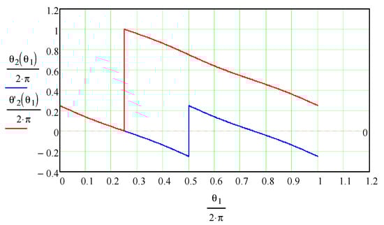
Figure 7.
The rotation angle of the driven element.
Thus, the application of an inverse trigonometric function of a single argument in describing the position of the driven element can lead to erroneous conclusions, as shown in Figure 7. At the interval the two relations give the same position of the driven element while on the domain between the two positions there is a delay of . The fact that the correct solution is the one given by the use of an inverse trigonometric function of two arguments will be justified in a subsequent section, by comparing the analytical results with the ones obtained using kinematic analysis software. The negative values of the transmission ratio show that when element 1 rotates in the positive direction of the axis , driven element 2 performs a rotation in the negative direction of the axis . Applying the derivative with respect to time (chain rule) of the relation (21) (or (22)), the transmission ratio of the mechanism can be obtained:
and is represented in Figure 8; it can be seen that the absolute value of the transmission ratio varies within the range .
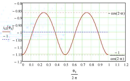
Figure 8.
Variation in the transmission ratio of the mechanism.
2.3. Establishing the Trajectory of the Contact Point from the Support Plane
In order to express the conditions (8)–(10), we note: (8)–(10)
By imposing the conditions (8)–(10), a system of three equations results, where the unknowns are the coordinates of the point :
The solutions of the system are the parametric coordinates of the point :
Squaring the equations of the system (29) and adding them member by member gives:
which represents the equation of a sphere of radius and with the center in the origin of the fixed system. In conclusion, the trajectory of the support point is a circle of radius , with the center in origin and placed in the support plane . The velocity of motion the point on the circular trajectory is constant, given by:
2.4. Finding the Motion from the Planar Joint between the Driving and Intermediate Elements
In order to specify the motion from the planar pair between elements 1 and 3, it is required to describe the position of a point from element 3 with respect to element 1 and of the position of the axes of frame 3 with respect to frame 1. The coordinates of the point from frame 3 in frame 1 are obtained using the relation:
where
In relation (33), all vectors are represented by the projections on the axes of the fixed system by the relations:
Relations (34) and (35) are obtained based on the physical meaning of the components of homogenous operators from relations (15) and (19). The components of the vectors and are given by Equations (28) and (25). The coordinate systems 1 and 3 have common axes and , respectively. Consequently, the relative motion of system 3 with respect to system 1 is a plane-parallel motion fully specified by the motion of the point in the plane and by the rotation angle of the axis or of axis with respect to axes and . Therefore:
After the calculus from relation (36) is made, the next relation is obtained:
By direct calculus, it can be shown that of the three components only the component from the axis is non-zero. It represents the displacement of point B along the straight-line trajectory, represented in Figure 9. By differentiating with respect to time, the velocity of point B results, as shown in Figure 10.
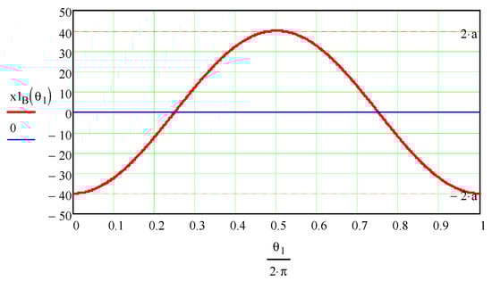
Figure 9.
Variation in the displacement of point B along the straight-line trajectory.
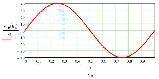
Figure 10.
The velocity of point B along the straight-line trajectory.
For the rotation between the plane with respect to the plane about the common normal , the following relation is applied:
The variation in this rotation is represented in Figure 11. The Equation (38) is derived numerically with respect to time to obtain the expression of the reduced angular velocity of the intermediate element with respect to the driving element. The variation in the angular velocity is presented in Figure 12.
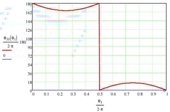
Figure 11.
The variation in the rotation angle .
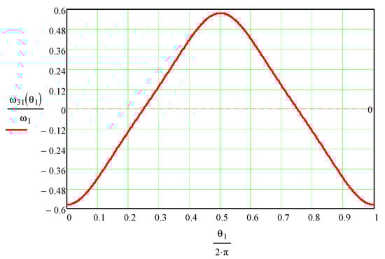
Figure 12.
Variation in the angular velocity .
When the velocity of a point from the intermediate element 3 is known with respect to the driving element 1 and the angular velocity of the intermediate element with respect to the driving element, using the Euler relation one can find the velocity of any point of element 3 with respect to the driving element:
2.5. Establishing the Relative Motion between the Intermediate and Driven Elements
Similarly, the coordinates of point from system 3 are expressed in frame 2 by the relation:
where
And
This relation (43) is written based on Equation (18). Comparing relation (43) with relation (34), one can see that the systems and have coinciding axes and and as a consequence, the relative motion between these systems can be fully described by the motion of point in plane and by the rotation of one of the axes or with respect to the axes of .
The trajectory of the point in plane is found using the relation:
After calculus is made in relation (44), one can observe that:
The physical meaning of relation (45) is that point B performs a planar trajectory relative to the driven element, as shown in Figure 13.
Figure 13.
Validation in the planar trajectory of point B with respect to the driven element.
The trajectory described by point in the plane is plotted in Figure 14 and its shape resembles a lemniscate enclosed by a rectangle.
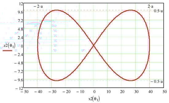
Figure 14.
Lemniscate-like trajectory of point in the plane .
In order to obtain the rotation motion of the intermediate element with respect to the final element, the next relation is applied:
The variation in this rotation for a complete rotation of the driving element is given in Figure 15. The time derivative of relation (46) leads to the expression of reduced relative angular velocity , whose variation is presented in Figure 16. From Figure 12 and Figure 16, it can be seen that for a complete rotation of the driving element, both angular velocities and present sign changes attesting that the intermediate element performs oscillatory motions, both with respect to the driving element and the driven element, respectively.
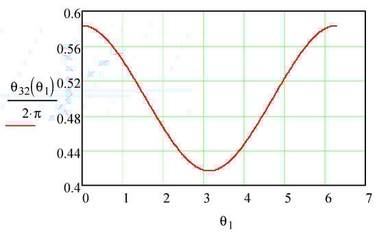
Figure 15.
Variation in the rotation of the intermediate element for a complete rotation of the driving element.
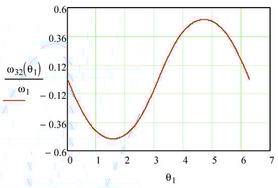
Figure 16.
Variation in the reduced relative angular velocity for a complete rotation of the driving element.
As mentioned previously, there are few references in the literature concerning planar joints. A significant example is given in [16] where the planar joint is modeled using a different method, namely the dual matrix method. However, in fact, this methodology transposes in dual form the condition that the planar pair is equivalated to a succession of prismatic–prismatic–revolute joints, and the H-D method is recovered.
3. Corroboration of Theoretical Results with a Numerical Simulation
3.1. Design of the Basic Mechanism
In order to validate the analytical results obtained above, the simplified mechanism was modeled in CATIA software. Specifically, the elements were modeled using the Wireframe and Surface Design modules, and then, the Assembly module was used for the assembly of the device, and the animation was performed in the DMU Kinematics module. The result is presented in Figure 17, where the circular trajectory of point in the support plane and the trajectories of points from two segments belonging to the intermediate element, parallel to coordinate axes, are shown. In Figure 18 and Figure 19 the trajectories of segments and are detailed and also compared to the analytical results, obtained in Mathcad, following the relations (33) and (41), respectively. An excellent quantitative concordance is attained from the comparison.
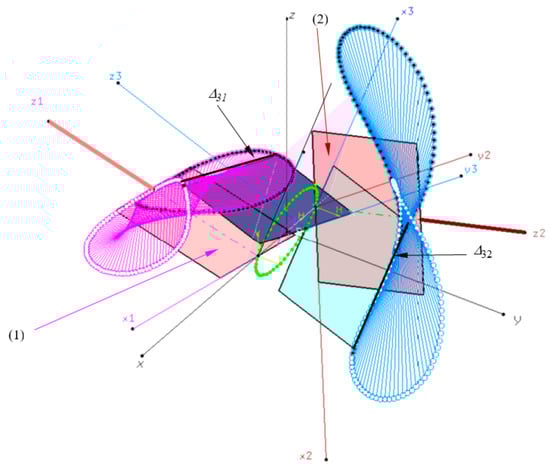
Figure 17.
Simplified model of the mechanism: trajectory of point B in the fixed plane (green circle); (1) is the plane of symmetry of driving element; (2) is the plane of symmetry of the driven element; and are segments attached to the elements (1) and (2) respectively.
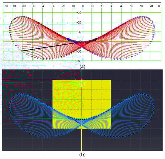
Figure 18.
Comparison between relative trajectories of a point situated on a segment of the intermediate element with respect to the driving element: (a) analytic trajectories–relations (33), of the points from the lines ; (b) CATIA simulation.
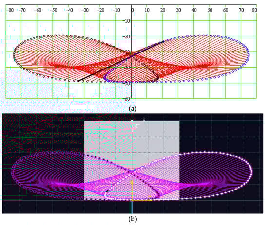
Figure 19.
Comparison between relative trajectories of a point situated on a segment of the intermediate element with respect to the driven element (a) analytic trajectory obtained with the relations (41); (b) CATIA simulation.
3.2. The Constructive Solution of the Proposed Coupling
To realize the transmission, the elements of the mechanisms should be designed to ensure the creation of the five kinematic pairs: revolute pairs, planar pairs, and the class 1 pair (the support between the intermediate element and the ground). The revolute pairs through which the first element and the final element are linked to the ground are straightforward to produce by mounting radial bearings on the surfaces and of the two elements. In Figure 20, the main components of the driving and driven elements are the two identical parts 1 and 2. In the bodies of these parts, two parallelepipedal channels are manufactured, with walls rigorously parallel to the axes of rotation of the parts. The main part of intermediate element 3 is crown 3 on which frontal faces are two parallelepipedal wedges 3b1 and 3b2, with the planes of symmetry reciprocally perpendicular. These wedges have the same width, theoretically identical to the width of the parallelepipedal channels from parts 1 and 2. By introducing the wedges 3b1 and 3b2 in the corresponding channels of parts 1 and 2, the two sliding fits are formed, realizing the planar pairs required by the structure of the mechanism. For achieving the pair of class 1, the major impediments are the revolute motions of elements 1 and 2 with respect to the ground. While rotating about the axes of the entrance and exit of the mechanism, respectively, these parts will generate the working spaces of the two elements. The presence of other parts in these working spaces could generate interference, and result in the locking of the mechanism. The proposed constructive solution is based on the fact that the points from the axes of rotation of elements 1 and 2 are fixed and can be considered as belonging to the ground. Additionally, as can be observed in Figure 20, the points inside any cylindrical hole coaxial to one of the two parts may be considered fixed points belonging to the ground. This explains the presence of the cylindrical plungers 1a and 1b, coaxial to the entering and exiting elements respectively, and having at one end a turntable. It is proposed that the pair of class 1 is created between the frontal surfaces of the turntables and the spherical surface 3a of the central body of the intermediate element 3, Figure 21. Obviously, the two contacts would conduct to a degree of mobility of the mechanism . Hence, the conclusion is that the center of sphere 3a must keep the same distance only with respect to one of the turntables.
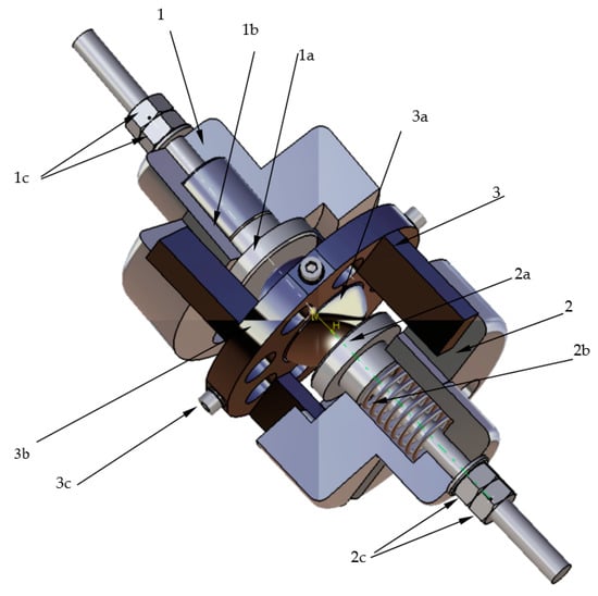
Figure 20.
Design of the proposed coupling.
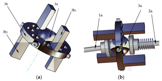
Figure 21.
The intermediate element: (a) design; (b) assembly for ensuring the contact from class 1 pair.
In Figure 20 the position of the turntable is fixed with the aid of rigid sleeve 1b of a length adequate to maintain the center of the sphere at the desired distance with respect to the body of part 1. Two screw nuts 1c block the plunger in the required position. For element 2, the rigid sleeve is replaced by helical spring 2b (Figure 21b), which, acting on the plunger 2a, will permit the axial displacement of the plunger with respect to the body of part 2. Thus, the class 1 pair is formed between spherical part 3a and the frontal surface of plunger 1a. An adequate running of the mechanism imposes the existence of the class 1 pair at any time. This requirement dictates that spring 2b is mounted with a minimum interference fit, made with screw nuts 2c. The screw nut tightening force can be obtained from dynamic analysis of the cam mechanism formed by the driving element 3a, the cam, and the follower realized by the plunger 2b.
The contact between spherical surface 3a and the frontal faces of plungers 1a and 2a are point Hertzian contacts, where important contact stresses occur that can lead to the rapid deterioration of the contacting surfaces, having as an immediate effect the improper running of the mechanism. This drawback can be mitigated as shown in [42], by introducing a shoe-type part between spherical surface 3a and the frontal face of plunger 1a, as shown in Figure 22.
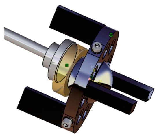
Figure 22.
Solution for diminishing the contact stresses and the wear from the higher pair.
By introducing the supplementary part between spherical surface 3a and plane surfaces 1a and 3a, all the pairs of the mechanism become lower pairs, having extremely high wear resistance. From the point of view of efficiency, the revolute pair, by which the driving and driven elements are joined to the ground, the employment of roller bearings is a solution. The friction from the higher pair can be decreased by manufacturing shoe part 4a from an antifriction material like graphite-filled bronze and through appropriate lubrication. Regarding the planar pairs, there is no technical solution for replacing the sliding friction with rolling friction. Similar to the case of higher pair, the diminishing of friction wear can be achieved by using antifriction pairs of materials like steel-bronze, PTFE (Teflon)-steel, etc.
The proposed coupling should be further improved because spatial couplings with crossed axes are quite rare, such as the patent of Segreti [43].
4. Discussions
The proposed coupling mechanism is entirely new among the spatial couplings transmitting the rotation motion between two shafts. The structural solution of the coupling resulted from the condition of transmission of rotation motion between two shafts, one driving and one driven, through an intermediate element. Within the practical solutions, a symmetrical structure of type RP1PR was the chosen option, such as the middle element completing a planar joint to each shaft and a class 1 pair with the ground. The choice of planar joints is based on the constructive straightforwardness and high reliability of these types of pairs. The existence of the class 1 pair between the intermediate element and the ground was imposed by the requirement that the degree of mobility of the mechanism is . To create the class 1 pair, it was required that the axis points of the two shafts are fixed and consequently can be considered as belonging to the ground. A stationary plane was fixed to one of the shafts, on which a spherical surface attached to the driving element is supported. Thus, the condition is met that the center of the spherical surface is permanently in a fixed plane attached to the ground and normal to the axis of the shafts (here, the driving shaft). A solution for diminishing the contact stresses from the sphere-plane concentrated point contact is presented, by placing a part between the spherical and plane surfaces, specially designed to replace the class 1 pair with two lower pairs of class 3: a spherical pair and a planar pair. The kinematic analysis of the planar pair requires obtaining the motions from planar joints, the relative trajectory of a point, and the angular velocity normal to the contacting surfaces. With these elements known, the absolute motion of any element of the transmission can then be expressed. The classical H-D methodology cannot be applied directly. It is shown that the method assumes equivalating the mechanism to another mechanism having a structure composed only of cylindrical, prismatic, and/or revolute pairs. By applying this methodology, complex trigonometrical systems result that can be solved only by numerical methods. For this solving procedure, the initialization demands a set of values corresponding to values close to a possible assembly solution for the actual mechanism, which is an extremely difficult task. The geometrical conditions (expressed in vector form) of constructing the joints from the structure of the mechanism, were applied. The components of the vectors from the relations of condition were expressed via the method of homogenous operators.
The proposed mechanism was also modeled in silico in order to obtain a numerical solution to validate the analytical results, comparing:
- the absolute trajectory of the center of the spherical surface of the intermediate element;
- the relative trajectories of points belonging to two segments from the middle part with respect to the driving element and final element, respectively.
A very good agreement was observed.
5. Conclusions
This work presents a completely new constructive solution of mechanical coupling that permits the transmission of motion between two axes positioned at a random angle in space, containing the succession of revolute–planar–point contact–planar–revolute joints, abbreviated RP1PR.
The kinematical analysis of the mechanism requires finding the motion from the revolute pair of the driven shaft, the trajectory of the spherical surface’s center, and the motions from the planar pairs.
The well-known method of Hartenberg and Denavit cannot be applied directly to the mechanism due to the presence in the structure of the planar pair and of the class 1 pair.
In order to overcome these difficulties, the geometrical conditions of creating the pairs from the structure of the mechanism, expressed in vector form were utilized.
With the purpose of validating the resulting theoretical relations, a scheme of the mechanism was modeled in numerical simulation software.
The excellent concordance between analytical and numerical results confirms that the obtained relations are correct.
The constructive solution of the mechanism is presented in a section of the paper, detailing the conception of the kinematical pairs and ways of diminishing contact stresses and wear. Compared to other structural solutions containing non-H-D pairs (spherical joints), the solution is more robust, reliable, and simpler from a technological point of view and more economic. From a constructive perspective, if a spherical joint risks locking, here, the three permitted motions are not limited.
The analytical results that were obtained could be, for future research, the basis for studies on the optimization of dimensions, with the task of reducing wear and improving the efficiency of transmission.
Author Contributions
Conceptualization, S.A., I.D. and M.-C.C.; methodology, I.D. and F.-C.C.; software, I.-C.R. and I.-A.D.; validation, I.-C.R. and M.-C.C.; investigation, I.-C.R. and I.-A.D.; writing—original draft preparation, S.A. and F.-C.C. writing—review and editing, I.D. and F.-C.C.; supervision, S.A. and M.-C.C. All authors have read and agreed to the published version of the manuscript.
Funding
This research received no external funding.
Data Availability Statement
The data presented in this study are available within the article.
Conflicts of Interest
The authors declare no conflict of interest.
References
- Uicker, J.J., Jr.; Pennock, G.R.; Shigley, J.E. Theory of Machines and Mechanisms, 4th ed.; Oxford University Press: New York, NY, USA, 2010; pp. 368–370. [Google Scholar]
- Molotnikov, V.; Molotnikova, A. Kinematic Analysis of Mechanisms. In Theoretical and Applied Mechanics; Springer Nature: Cham, Switzerland, 2023; pp. 299–310. [Google Scholar] [CrossRef]
- Hunt, K.H. Kinematic Geometry of Mechanisms; Oxford University Press: Oxford, UK, 1990; pp. 30–51. [Google Scholar]
- McCarthy, J.M. Introduction in Theoretical Kinematics, 3rd ed.; MIT Press: Cambridge, MA, USA, 2018; pp. 103–108. [Google Scholar]
- Roupa, I.; Gonçalves, S.B.; Silva, M.T. Kinematics and dynamics of planar multibody systems with fully Cartesian coordinates and a generic rigid body. J. Mech. Mach. Theory 2023, 180, 105134. [Google Scholar] [CrossRef]
- Inurritegui, A.; Larranaga, J.; Arana, A.; Ulacia, U. Numerical-experimental analysis of highly crowned spherical gear couplings working at high misalignment angles. J. Mech. Mach. Theory 2023, 183, 105260. [Google Scholar] [CrossRef]
- Wu, K.; Liu, Z.; Ding, Q. Vibration responses of rotating elastic coupling with dynamic spatial misalignment. J. Mech. Mach. Theory 2020, 151, 103916. [Google Scholar] [CrossRef]
- Cao, A.; Jing, Z.; Ding, H. A general method for kinematics analysis of two-layer and two-loop deployable linkages with coupling chains. J. Mech. Mach. Theory 2020, 152, 103945. [Google Scholar] [CrossRef]
- Baigunchekov, Z.; Laribi, M.A.; Carbone, G.; Mustafa, A.; Amanov, B.; Zholdassov, Y. Structural-Parametric Synthesis of the RoboMech Class Parallel Mechanism with Two Sliders. Appl. Sci. 2021, 11, 9831. [Google Scholar] [CrossRef]
- Zhang, J.; Ng, N.; Scott, C.E.H.; Blyth, M.J.G.; Haddad, F.S.; Macpherson, G.J.; Patton, J.T.; Clement, N.D. Robotic arm-assisted versus manual unicompartmental knee arthroplasty. Bone Joint J. 2022, 104, 541–548. [Google Scholar] [CrossRef] [PubMed]
- McCarthy, J.M.; Soh, G.S. Geometric Design of Linkages; Springer: Berlin/Heidelberg, Germany, 2010; pp. 253–279. [Google Scholar]
- Hartenberg, R.; Denavit, J. Kinematic Synthesis of Linkages, 1st ed.; McGraw-Hill Inc.: New York, NY, USA, 1964; pp. 343–368. [Google Scholar]
- Alaci, S.; Pentiuc, R.D.; Doroftei, I.; Ciornei, F.C. Use of dual numbers in kinematical analysis of spatial mechanisms. Part II: Applying the method for the generalized Cardan mechanism. IOP MSE 2019, 568, 12032. [Google Scholar] [CrossRef]
- Angeles, J. Spatial Kinematic Chains: Analysis-Synthesis-Optimization; Springer: Berlin/Heidelberg, Germany, 1982; pp. 189–218. [Google Scholar]
- Ciornei, F.C.; Amarandei, D.; Alaci, S.; Romanu, I.C.; Baesu, M. On direct coupling of two shafts. Part 2: Kinematical analysis. Tehnomus J. 2017, 24, 281–285. [Google Scholar]
- Fischer, I. Dual-Number Methods in Kinematics, Statics and Dynamics; CRC Press: New York, NY, USA, 1999; pp. 54–95. [Google Scholar]
- Alaci, S.; Pentiuc, R.D.; Ciornei, F.C.; Buium, F.; Rusu, O.T. Kinematics analysis of the swash plate mechanism. IOP MSE 2019, 568, 012017. [Google Scholar]
- Angeles, J. Rational Kinematics; Springer: New York, NY, USA, 1998; pp. 12–34. [Google Scholar]
- Uicker, J.J., Jr.; Denavit, J.; Hartenberg, R.S. An Iterative Method for the Displacement Analysis of Spatial Mechanisms. J. Appl. Mech. 1964, 31, 309–314. [Google Scholar] [CrossRef]
- Selig, J.M. On the Plane Symmetric Bricard Mechanism. In Advances in Robot Kinematics 2020 (Springer Proceedings in Advanced Robotics Book 15); Lenarčič, J., Siciliano, B., Eds.; Springer Nature: Cham, Switzerland, 2021; pp. 73–81. [Google Scholar]
- Seherr-Thoss, H.C.; Schmelz, F.; Aucktor, E. Universal Joints and Driveshafts. Analysis, Design, Applications, 2nd ed.; Springer: Berlin/Heidelberg, Germany, 2006; pp. 53–79. [Google Scholar]
- Inurritegui, A.; Larranaga, J.; Arana, A.; Ulacia, U. Load distribution and tooth root stress of highly crowned spherical gear couplings working at high misalignment angles. J. Mech. Mach. Theory 2023, 179, 105104. [Google Scholar] [CrossRef]
- Luzi, L.; Sancisi, N.; Parenti-Castelli, V. The Potential of the 7R-R Closed Loop Mechanism to Transfer Motion Between Two Shafts with Varying Angular Position. In Interdisciplinary Applications of Kinematics. Mechanisms and Machine Science; Kecskeméthy, A., Geu Flores, F., Carrera, E., Elias, D., Eds.; Springer: Cham, Switzerland, 2019; Volume 71, pp. 185–195. [Google Scholar] [CrossRef]
- Lobontiu, N.; Hunter, J.; Keefe, J.; Westenskow, J. Tripod mechanisms with novel spatial Cartesian flexible hinges. J. Mech. Mach. Theory 2022, 167, 104521. [Google Scholar] [CrossRef]
- Yoon, K.; Cho, S.-M.; Kim, K.G. Coupling Effect Suppressed Compact Surgical Robot with 7-Axis Multi-Joint Using Wire-Driven Method. Mathematics 2022, 10, 1698. [Google Scholar] [CrossRef]
- Litvin, F.L.; Fuentes, A. Gear Geometry and Applied Theory; Cambridge University Press: Cambridge, UK, 2004; pp. 441–474. [Google Scholar]
- Vullo, V. Gears, Volume 1: Geometric and Kinematic Design; Springer: Cham, Switzerland, 2021; pp. 139–151. [Google Scholar]
- Gonzales-Palacios, M.A.; Angeles, J. Cam Synthesis; Springer: Dordrecht, The Netherland, 1993; pp. 37–53. [Google Scholar]
- Alaci, S.; Ciornei, F.C.; Amarandei, D.; Baesu, M.; Mihaila, D. On direct coupling of two shafts. Part 1: Structural considerations. Tehnomus J. 2017, 24, 277–280. [Google Scholar]
- Akbil, E.; Lee, T.W. On the motion characteristics of tripode joints. Part 1: General case; Part 2: Applications. ASME J. Mech. Transm. Autom. Des. 1984, 106, 228–241. [Google Scholar] [CrossRef]
- Johnson, K.L. Contact Mechanics; Cambridge University Press: Cambridge, UK, 1985; pp. 84–106. [Google Scholar] [CrossRef]
- Hills, D.A.; Nowell, D.; Sackfield, A. Mechanics of Elastic Contacts; Elsevier Butterworth-Heinemann: Oxford, UK, 1993; pp. 198–226. [Google Scholar]
- Popov, V.L. Contact Mechanics and Friction. Physical Principles and Applications; Springer: Berlin/Heidelberg, Germany, 2010; pp. 55–69. [Google Scholar]
- Gladwel, G.M.L. Contact Problems in the Classical Theory of Elasticity; Sijthoff & Noordhoff: Hague, The Netherlands, 1980; p. 716. [Google Scholar]
- Alaci, S.; Buium, F.; Ciornei, F.-C.; Dobincă, D.-I. Tetrapod coupling. Mech. Mach. Sci. 2018, 57, 349–356. [Google Scholar] [CrossRef]
- Inurritegui, A.; Larranaga, J.; Arana, A.; Ulacia, U. Spherical gear coupling design space analysis for high misalignment applications. Mech. Mach. Theory 2022, 173, 104837. [Google Scholar] [CrossRef]
- Hayes, M.J.D.; Rotzoll, M.; Bucciol, Q.; Copeland, A.A. Planar and spherical four-bar linkage vi−vj algebraic input–output equations. J. Mech. Mach. Theory 2023, 182, 105222. [Google Scholar] [CrossRef]
- EN ISO 3952-1; Kinematic Diagrams—Graphical Symbols. Part 1. The European Standard: Geneva, Switzerland, 2019; pp. 1–25.
- Sclater, N. Mechanisms and Mechanical Devices Sourcebook, 5th ed.; McGraw Hill: New York, NY, USA, 2011; pp. 109–110. [Google Scholar]
- Yoshikawa, T. Foundations of Robotics: Analysis and Control; MIT Press: Cambridge, MA, USA, 2003; pp. 259–262. [Google Scholar]
- Maxfield, B. Engineering with Mathcad; Butterworth-Heinemann, Elsevier: Oxford, UK, 2006; pp. 287–289. [Google Scholar]
- Alaci, S.; Ciornei, F.C.; Filote, C. Considerations upon a New Tripod Joint Solution. Mechanika 2013, 19, 567–574. [Google Scholar] [CrossRef]
- Segreti, A. Mechanism for the Transmission of Rotary Movement between two Shafts having Non-Parallel, Non-Coplanar Axes. U.S. Patent WO 02/103220 A2, 27 December 2002. [Google Scholar]


Disclaimer/Publisher’s Note: The statements, opinions and data contained in all publications are solely those of the individual author(s) and contributor(s) and not of MDPI and/or the editor(s). MDPI and/or the editor(s) disclaim responsibility for any injury to people or property resulting from any ideas, methods, instructions or products referred to in the content. |
© 2023 by the authors. Licensee MDPI, Basel, Switzerland. This article is an open access article distributed under the terms and conditions of the Creative Commons Attribution (CC BY) license (https://creativecommons.org/licenses/by/4.0/).