Numerical Solution of Fractional Models of Dispersion Contaminants in the Planetary Boundary Layer

Abstract

In this study, a numerical solution for degenerate space–time fractional advection–dispersion equations is proposed to simulate atmospheric dispersion in vertically inhomogeneous planetary boundary layers. The fractional derivative exists in a Caputo sense. We establish the maximum principle and a priori estimates for the solutions. Then, we construct a positivity-preserving finite-difference scheme, using monotone discretization in space and L1 approximation on the non-uniform mesh for the time derivative. We use appropriate grading techniques for the time–space mesh in order to overcome the boundary degeneration and weak singularity of the solution at the initial time. The computational results are demonstrated on the Gaussian fractional model as well on the boundary layers defined by height-dependent wind flow and diffusitivity, especially for the Monin–Obukhov model.

1. Introduction

Nowadays, environmental problems are very important in our world, and their importance will increase in the future. The high levels of pollution in the air and the contamination of groundwater and soil may cause the damage of plants, animals and humans. Many models that study the physical processes in the atmospheric boundary layer (ABL) are generally described by PDEs; see, for example, [1,2,3,4]. The pollutants under atmosphere turbulence lead to anomalous diffusion [2,3,5,6]. Refs. [3,5,6,7,8,9] discuss the relevance of using the fractional derivative in studying dispersion contaminants in the planetary boundary layer (PBL). The authors of [5,10], solving a simple fractional derivative equation, describing the steady-state spatial distribution of a non-reactive pollutant and comparing the results with those of real experiments, show some advantageous traits of the fractional model. In contrast to classical integer differential equations, the fractional-order equations are more adequate for this modeling.

A lot of experimental work have been performed to find realistic forms of wind speeds and diffusitivities, such as

$$\mathrm{u}\approx z^{\beta }\mathrm{and}{k}_z=z^{\gamma },$$

where z denotes height above ground and $\beta >0$ and $\gamma >0$ are constants. In [1,2,3,5,6,11,12,13], the stable boundary layers are defined by height-dependent wind flow and diffusitivity

$$\mathrm{u}\left(z\right)=\frac{4-7u_{*}}{\kappa L}z,k_z=\frac{\kappa u_{*}L}{4.7}{\left(1-\frac{z}{Z}\right)}^2\mathrm{and}{k}_z=z^{\gamma },$$

(1)

respectively. Here, $\kappa$ is Karman’s constant, $u_{*}$ is the friction velocity, L is the Monin–Obukhov stability length and Z is the boundary layer height.

The Monin–Obukhov theory of the ABL [5,14] is applied, and for transversal eddy-diffusivity, the expression is often used

$$k(z,t)=\phi \left(t\right)z(Z-z)(1-22\frac{z}{L}),$$

(2)

where $L<0$ is the Monin–Obukhov length, and $\phi \left(t\right)$ is the measured velocity; see, for example, [15,16,17].

In [7,11], the wind velocity is assumed to be horizontal and spatially uniform within each horizontal panel. Then, the following well-known power–law form [1,11] is given by

$$\mathrm{w}(z,t)=\tilde{u}-u_r\left(t\right){\left(\frac{z}{z_r}\right)}^{\delta },$$

(3)

where $u_r\left(t\right)$ represents the measured wind velocity at a reference height $z_r>0$, and $\delta >0$ is a fitting parameter, related to the intensity of the turbulence and ranges between 0.2 and 0.4 [11].

Refs. [3,5,6,7,8,18] developed the modeling of pollutant transport under turbulence with Caputo and Riemann–Liouville fractional derivatives that present the anomalous diffusion phenomena. Here, we also include realistic forms of the vertical diffusion coefficient and windfield.

The dispersion model is described by the following fractional advection–diffusion PDE:

$$\begin{array}{c}{D}_0^{\alpha }u=k(z,t)\frac{{\partial }^{2}u}{\partial z^2}+p(z,t)\frac{\partial u}{\partial z}+q(z,t)u+f(z,t),(z,t)\in Q_T=\mathsf{\Omega }\times (0,T),\mathsf{\Omega }=(0,Z),\hfill \end{array}$$

(4)

$$\begin{array}{c}u(z,0)=u_0\left(z\right),(z,t)\in \overline{\mathsf{\Omega }}=[0,Z].\hfill \end{array}$$

(5)

Here,

$$k(z,t)=K\left(z\right)\phi \left(t\right),k(0,t)=0,k(l,t)=0,k(z,t)\ge \tilde{k}>0,z\in \mathsf{\Omega },$$

(6)

and $D_0^{\alpha }u$ is the left Caputo derivative of order $\alpha$, $0<\alpha <1$ [19,20,21].

The computational domain is represented by $\mathsf{\Omega }$ and it is within ABL.

Classical (integer-order) atmospheric dispersion problems both with constant and non-constant eddy diffusivity and wind speed profiles are well studied in the literature [1,4,11,13,14,15,16,22,23,24,25,26,27,28]. The effect of the boundary degeneration, arising from power–law modeling using the Monin–Obukhov [29] similarity theory and its impact on the accuracy of the numerical solution, is not sufficiently investigated.

Ref. [12] obtains a semi-analytical model to simulate the distribution of contaminants in a turbulent flow. A numerical approach, based on the locally one-dimensional technique, is proposed. The well posedness of the variational form of the classical atmospheric dispersion problem with degenerate vertical diffusion in weighted Sobolev spaces is investigated in [14]. Ref. [16] considers a numerical model to study the dispersion of pollutants in the ABL with wind speed and eddy diffusivity profiles, dependent on the atmospheric stability condition. The authors of [26] construct and analyze artificial boundary conditions in order to numerically solve the advection–diffusion problem of air and water pollution. The monotonicity- and positivity-preserving properties of the solution are also discussed. In [23], the authors numerically study a problem, modeling the secondary and primary pollutants and their removal mechanism in the city region. A fitted finite volume method for solving classical air pollution models with space degenerate diffusion is constructed and analyzed in [28,30].

The finite volume method with Godunov time splitting in an advection–dispersion model with height-dependent advection and diffusion coefficients is constructed in [11] for estimating the emissions of airborne particulates from point sources. The standard Gaussian plume model is also used in [17] to investigate the transport of contaminants in the air due to turbulent diffusion and wind advection and to determine emission source rates. The authors of [15] propose a genetic algorithm for source identification in the atmospheric dispersion problem with power–law vertical turbulent diffusion.

Fractional atmospheric models are introduced and analyzed in [3,5,6,7,8,18,31]. In [3,5,6], the fractional differential equation in the longitudinal and vertical directions is used to derive the concentration distribution of pollutants in the PBL. They propose an analytical solution for the steady-state problem. The authors compare the results with the one obtained by the traditional Gaussian model and report a very good fitting of the fractional model to the experimental data. Closed-form solutions for solving the fractional dispersion problem under a variable atmospherical hypothesis in a vertical non-homogeneous PBL is proposed in [8]. Better performance of the fractional-order model in comparison with that of the integer order is observed. Ref. [7] investigates the fractional-order problem to simulate secondary pollutant dispersion in PBL, and the influence of the memory effect on primary and secondary pollutants is studied. By the numerical tests, based on the semi-analytical solution, the relevance of the proposed model and agreement with physical processes is illustrated. Authors of [32] develop an unconditionally stable finite difference method on non-uniform meshes for time-fractional advection–diffusion equations.

A system of fractional differential equations, describing the amount of pollution in lakes connected with rivers is introduced in [33]. Results for the existence and regularity of the solution are obtained, and a high-order numerical method is introduced.

Ref. [31] constructs an exponential difference scheme for the fractional-order advection–diffusion problem for the dispersion of pollutants with discontinuous diffusivity profiles. Refs. [18,30] proposes numerical methods for identifying the vertical diffusion coefficient and concentration source in a fractional air-pollution model with a power vertical diffusion coefficient.

The influence of the fractional parameter on the fluid motion and the effect on the boundary layer in time-fractional differential equations is studied in [34]. Authors determine analytical solutions for the velocity components, applying the generalized method of the separation of variables and the Laplace transform method.

Inverse problems for the identification coefficient, source, initial value, boundary conditions, etc., in a time-fractional diffusion equation are investigated in many papers; see, for example, [35,36,37,38,39]. Recently, there has been progress made on solving inverse tempered fractional diffusion problems modeling complex multi-scale problems and anomalous transport phenomena. Ref. [40] proposes a meshless numerical procedure for solving the inverse tempered fractional diffusion equation. The uniqueness of the solution of two inverse problems for reconstructing the history of a function based on its value and source term in a generalized fractional diffusion equation is proved in [41]. Inverse problems for identifying space-dependent components in a source term and linear reaction term in a generalized subdiffusion equation are studied in [42]. The authors prove the existence, uniqueness and stability of the solution.

In this work, we propose and analyze a new unconditional positivity-preserving approach for handling boundary degeneration in fractional atmospheric flow problems. We extend some results proposed in the conference report [43].

The the remainder of this paper is organized as follows. A discussion on fractional calculus is presented in Section 2. In Section 3, some basic results of the fractional calculus are given, and the maximum principle is proved for the Cauchy problem of the degenerate parabolic Equation (4). In Section 4, some a priori estimates of the initial-boundary value problem (4)–(6) are obtained. In Section 5, we construct a monotone numerical scheme, which handles the spatial degeneration, and in Section 6, we establish the unconditional positivity-preserving property of the proposed discretization. Some results obtained for the one-dimensional case are extended to the two-dimensional case in Section 7. Numerical experiments are presented in Section 8, and the paper is closed with some conclusions in the last section.

2. Preliminaries

In this section, we discuss fractional operators and give some basic statements, which are useful for our further analysis.

First, we define Riemann–Liouville fractional integrals and fractional derivatives of the real order $\alpha >0$ [20,21].

Let $[a,b]$ be a finite interval on the real axis. The left and right Riemann–Liouville fractional integrals of order $\alpha$ are

$$\begin{array}{ccc}& & {}^{RL}{I}_{a+}^{\alpha }g\left(t\right)=\frac{1}{\Gamma \left(\alpha \right)}\underset{a}{\overset{t}{\int }}\frac{g\left(\eta \right)d\eta }{{(t-\eta )}^{1-\alpha }},t>a,\hfill \\ & & {}^{RL}{I}_{b-}^{\alpha }g\left(t\right)=\frac{1}{\Gamma \left(\alpha \right)}\underset{t}{\overset{b}{\int }}\frac{g\left(\eta \right)d\eta }{{(\eta -t)}^{1-\alpha }},t<b,\hfill \end{array}$$

where $\Gamma (·)$ is the gamma function [20,21].

Consequently, the left and right Riemann–Liouville fractional derivatives of order $\alpha$ are defined by

$$\begin{array}{ccc}& & {}^{RL}{D}_{a+}^{\alpha }v\left(t\right)={\left(\frac{d}{dt}\right)}^n{}^{RL}{I}_{a+}^{n-\alpha }v\left(t\right),t>a\hfill \\ & & {}^{RL}{D}_{b-}^{\alpha }v\left(t\right)={\left(-\frac{d}{dt}\right)}^n{}^{RL}{I}_{b-}^{n-\alpha }v\left(t\right),t<b,\hfill \end{array}$$

where $n=\alpha +1$ for $\alpha \notin \mathbb{N}$ and $n=\alpha$ for $\alpha \in \mathbb{N}$. Note that in this case, ${}^{RL}{D}_{a+}^{0}v\left(t\right)={}^{RL}{D}_{b-}^{0}v\left(t\right)=v\left(t\right)$ and ${}^{RL}{D}_{a+}^{n}v\left(t\right)=v^{\left(n\right)}\left(t\right)$, ${}^{RL}{D}_{b-}^{n}v\left(t\right)={(-1)}^n{v}^{\left(n\right)}\left(t\right)$, where $v^{\left(n\right)}\left(t\right)$ is the classical derivative of $v\left(t\right)$ of order n.

The left and right Caputo fractional derivatives are closely related to the corresponding Riemann–Liouville fractional derivatives, and they are defined as follows [19,20,21]:

$$\begin{array}{ccc}& & {}^C{D}_{a+}^{\alpha }v\left(t\right)=\frac{1}{\Gamma (n-\alpha )}\underset{a}{\overset{t}{\int }}\frac{v^{\left(n\right)}\left(\eta \right)d\eta }{{(t-\eta )}^{\alpha -n+1}}={}^{RL}{I}_{a+}^{n-\alpha }{D}^{n}v\left(t\right),\hfill \\ & & {}^C{D}_{b-}^{\alpha }v\left(t\right)=\frac{{(-1)}^n}{\Gamma (n-\alpha )}\underset{t}{\overset{b}{\int }}\frac{v^{\left(n\right)}\left(\eta \right)d\eta }{{(\eta -t)}^{\alpha -n+1}}={(-1)}^n{}^{RL}{I}_{b-}^{n-\alpha }{D}^{n}v\left(t\right).\hfill \end{array}$$

where $n=\alpha +1$ for $\alpha \notin \mathbb{N}$ and $n=\alpha$ for $\alpha \in \mathbb{N}$ and $D=\frac{d}{dt}$.

The well-known relations between Caputo and Riemann–Liouville fractional derivatives [19,20,21] are simplified in the case of $0<\alpha <1$, namely

$$\begin{array}{ccc}& & {}^C{D}_{a+}^{\alpha }v\left(t\right)={}^{RL}{D}_{a+}^{\alpha }(v\left(\eta \right)-v\left(a\right))\left(t\right),{}^C{D}_{b-}^{\alpha }v\left(t\right)={}^{RL}{D}_{b-}^{\alpha }(v\left(\eta \right)-v\left(b\right))\left(t\right).\hfill \end{array}$$

In the following, for $a=0$, we will use the notation $D_0^{\alpha }v\left(t\right):={}^C{D}_{0+}^{\alpha }v\left(t\right)$ for the left Caputo derivative and in particular, in Equation (4), we have

$$D_0^{\alpha }u(z,t)={}^C{D}_{0+}^{\alpha }u(z,t)=\frac{1}{\Gamma (1-\alpha )}\underset{0}{\overset{t}{\int }}\frac{\partial u(z,\eta )}{\partial \eta }{(t-\eta )}^{-\alpha }d\eta ,0<\alpha <1.$$

Further, we will employ the following results.

Lemma 1

([44]). For any absolutely continuous function $y\left(t\right)$ on $[0,T]$, one has the inequality

$$y\left(t\right)D_0^{\alpha }y\left(t\right)\ge \frac{1}{2}{D}_0^{\alpha }{y}^2\left(t\right),0<\alpha <1.$$

Lemma 2

([44]). Let the absolutely continuous function $y\left(t\right)$ satisfy the inequality

$$D_0^{\alpha }y\left(t\right)\le C_{1}y\left(t\right)+C_2\left(t\right),0<\alpha \le 1,$$

for almost all $t\in [0,T]$, where $C_1>0$ is a constant and $C_2\left(t\right)$ is an integrable non-negative function on $[0,T]$. Then,

$$y\left(t\right)\le y\left(0\right)E_{\alpha }\left(C_1{t}^{\alpha }\right)+\Gamma \left(\alpha \right)E_{\alpha ,\alpha }\left(C_1{t}^{\alpha }\right)D_0^{-\alpha }{C}_2\left(t\right),$$

where $E_{\alpha }\left(z\right)={\displaystyle \sum _{n=0}^{\infty }}{z}^n/\Gamma (\alpha n+1)$ and $E_{\alpha ,\mu }\left(z\right)={\displaystyle \sum _{n=0}^{\infty }}{z}^n/\Gamma (\alpha n+\mu )$ are Mittag–Leffler functions.

Lemma 3

([45]). Let a function $y\left(t\right)\in W_t^1\left((0,t]\right)\cap C\left([0,T]\right)$ attain its maximum over the interval $[0,T]$ at the point $t_0\in (0,T]$. Then

$$D_0^{\alpha }u\left(t_0\right)\ge 0,0<\alpha <1.$$

3. Maximum Principle

Following the physical models, described in the previous section, we investigate the non-negativity of the solutions of the problem (4)–(6).

On the basis of the results in [46] we may formulate the following statement.

Lemma 4.

Suppose that $y\left(t\right)\in C^1\left([0,T]\right)$ and

(i)$f\left(t\right)<f\left(t_0\right)$ for all $0\le t\le t_0\le T$,

(ii)$D_0^{\alpha }u\left(t_0\right)=0$,

then $f\left(t\right)=f\left(t_0\right)$ for all $0\le t\le t_0$.

Lemma 5 (Maximum principle).

Assume the formulation (4)–(6) holds and $-q(z,t)\ge \tilde{q}>0$, $u(z,t)\in C^{2,1}\left(Q_T\right)\cap C\left({\overline{Q}}_T\right)$. If

$$Lu=D_0^{\alpha }u-k(z,t)\frac{{\partial }^{2}u}{\partial z^2}-p(z,t)\frac{\partial u}{\partial z}-q(z,t)u\le 0,$$

then $u(z,t)$ can only attain the positive maximum at the non-degenerate parabolic boundary

$${\Gamma }_n=\left\{(z,t)\right|t=0,z\in (0,Z)\}.$$

Proof. 

First, let us assume that $u(z,t)$ attains the the positive maximum M at the internal point $M_0(z,t)\in Q_T$, i.e.,

$$u(z_0,t_0)=\underset{{\overline{Q}}_T}{max}u(z,t)=M>0.$$

Then, this implies

$$\frac{\partial u}{\partial z}{|}_{M_0}=0\mathrm{and}\frac{{\partial }^{2}u}{\partial z^2}\le 0\mathrm{for}z\in (0,Z).$$

Additionally, in view of Lemmas 3 and 4, we have

$$D_0^{\alpha }u{|}_{M_0}=0\mathrm{for}{t}_0<T,D_0^{\alpha }u{|}_{M_0}\ge 0\mathrm{for}{t}_0=T.$$

Hence, we find

$$Lu{|}_{M_0}=-q(z_0,t_0)M\ge \tilde{q}M>0,$$

which is a contradiction of the lemma.

Next, we show that $u(z,t)$ cannot attain the positive maximum at the generate boundaries

$$\{z=0,0<t\le T\}\cup \{z=Z,0<t\le T\}.$$

Without loss of generality, we assume that $u(z,t)$ attains its positive maximum M at the point $M_1(0,t_1)$, $0<t_1\le T$. Then, we have

$$D_0^{\alpha }u{|}_{M_1}=0,0<t_1<T;D_0^{\alpha }u{|}_{M_1}\ge 0,t_1=T.$$

Moreover, from

$$k(0,t)=0,k(z,t)>0,(z,t)\in Q_T,$$

it follows that $\frac{\partial k}{\partial z}(0,t)\ge 0$. Since $u(0,t_1)=M$ is a maximum, we have

$$u(z,t_1)\le u(0,t_1)\mathrm{for}\forall z\in (0,Z),$$

which implies

$$\frac{\partial u}{\partial z}(0,t_1)=\underset{z\to 0^{+}}{lim}\frac{u(z,t_1)-u(0,t_1)}{z}\le 0.$$

Therefore, we have

$$\begin{array}{ccc}\hfill Lu{|}_{M_1}& =& \frac{\partial u}{\partial t}{|}_{M_1}-k(0,t_1)\frac{{\partial }^{2}u}{\partial z^2}{|}_{M_1}-\left(p(0,t_1)-\frac{\partial k(0,t_1)}{\partial z}\right)\frac{\partial u}{\partial z}{|}_{M_1}-\frac{\partial k(0,t_1)}{\partial z}\frac{\partial u}{\partial z}{|}_{M_1}\hfill \\ & & -q(0,t_1)u{|}_{M_1}\ge \tilde{q}M>0,\hfill \end{array}$$

which also contradicts the assumption of the lemma.

With similar arguments, one can show that $u(z,t)$ cannot attain the positive maximum at the right degenerate boundary $\{z=Z,0<t\le T\}$. □

Corollary 1.

Suppose that the assumptions of Lemma 5 hold, but $Lu\ge 0$; then, $u(z,t)$ only attain its negative minimum at the non-degenerate parabolic boundary.

Theorem 1.

Suppose that the assumptions of Lemma 5 hold without the sign of $Lu$ defined. Then, for $u(z,t)$ we have the following estimate:

$$\underset{{\overline{Q}}_T}{max}u\le max\left\{\frac{1}{\tilde{q}}\underset{Q_T}{sup}\left|f\right|,\underset{\mathsf{\Omega }}{sup}\left|u_0\right|\right\}.$$

Proof. 

Let

$$M=max\left\{\frac{1}{\tilde{q}}\underset{Q_T}{sup}\left|f\right|,\underset{\mathsf{\Omega }}{sup}\left|u_0\right|\right\}$$

and $v(z,t)=M\pm u(z,t)$. One can easily check that

$$Lv=LM\pm Lu=Mq(z,t)\pm f(z,t)\ge 0,v(z,0)=M\pm u_0\left(z\right)\ge 0.$$

From Corollary 1, we have $v(z,t)\ge 0$, $(z,t)\in {\overline{Q}}_T$. Hence $\underset{{\overline{Q}}_T}{max}\left|u\right|\le M$. □

4. A Priori Estimates for the Solutions

We rewrite Equation (4) in the semidivergent form

$$D_0^{\alpha }u=\mathcal{L}u+f(z,t),\mathcal{L}u=\frac{\partial }{\partial z}\left(k(z,t)\frac{\partial u}{\partial z}\right)+\left(p(z,t)-\frac{\partial k(z,t)}{\partial z}\right)\frac{\partial u}{\partial z}+q(z,t)u.$$

(7)

The coefficient at $\frac{\partial u}{\partial z}$ plays a key role in the discretization of the boundary conditions. Namely, if

$$p(0,t)-\frac{\partial k(0,t)}{\partial z}\ge 0\mathrm{and}p(Z,t)-\frac{\partial k(Z,t)}{\partial z}\le 0\mathrm{for}t\in [0,T],$$

(8)

no boundary conditions can be imposed. If

$$p(0,t)-\frac{\partial k(0,t)}{\partial z}<0\mathrm{for}t\in [0,T],$$

(9)

a boundary conditions at $z=0$, such as

$$u(0,t)={\phi }_l\left(t\right)\mathrm{for}t\in [0,T],$$

(10)

must be imposed in order to have a unique solution. Further, if

$$p(Z,t)-\frac{\partial k(Z,t)}{\partial z}>0\mathrm{for}t\in [0,T],$$

(11)

then, at $z=Z$ a boundary conditions

$$u(Z,t)={\phi }_r\left(t\right)\mathrm{for}t\in [0,T],$$

(12)

must be imposed. This discussion provides the well posedness of the initial-boundary value problems, as defined.

Theorem 2.

Let $k(z,t)\in C^{1,0}\left({\overline{Q}}_T\right)$, $p(z,t)$, $q(z,t)$, $f(z,t)\in C\left({\overline{Q}}_T\right)$, $k(z,t)$ is defined by (6) and $q(z,t)\le 0$ everywhere in ${\overline{Q}}_T$. If the solution as defined above exists in $C^{2,1}\left({\overline{Q}}_T\right)$, then it is unique and stable with respect to the initial value $u_0\left(z\right)$, right-hand side $f(z,t)$, and the boundary values of ${\phi }_l\left(t\right)$ and ${\phi }_r\left(t\right)$.

Proof. 

We multiply the Equation (7) by $2u$ to derive

$$\begin{array}{ccc}\hfill 2u{D}_0^{\alpha }u& =& 2\frac{\partial }{\partial z}\left(ku\frac{\partial u}{\partial z}\right)+\left(p-\frac{\partial k}{\partial z}\right)\frac{\partial u^2}{\partial z}-2k{\left(\frac{\partial u}{\partial z}\right)}^2+2q{u}^2+2fu\hfill \\ & =& 2\frac{\partial }{\partial z}\left(ku\frac{\partial u}{\partial z}\right)+\frac{\partial }{\partial z}\left[\left(p-\frac{\partial k}{\partial z}\right)u^2\right]-2k{\left(\frac{\partial u}{\partial z}\right)}^2\hfill \\ & & +\left(\frac{{\partial }^{2}k}{\partial z^2}-\frac{\partial p}{\partial z}+2q\right)u^2+2fu.\hfill \end{array}$$

(13)

Integrating (13) with respect to z on the interval $[0,Z]$, we obtain

$$\begin{array}{c}\hfill \begin{array}{cc}\hfill 2\underset{0}{\overset{Z}{\int }}u{D}_0^{\alpha }udz=& 2\left(ku\frac{\partial u}{\partial z}\right){|}_0^Z+{\left[\left(p-\frac{\partial k}{\partial z}\right)u^2\right]}_0^Z-2\underset{0}{\overset{Z}{\int }}k{\left(\frac{\partial u}{\partial z}\right)}^{2}dz\hfill \\ & +\underset{0}{\overset{Z}{\int }}\left(\frac{{\partial }^{2}k}{\partial z^2}-\frac{\partial p}{\partial z}+2q\right)u^{2}dz+2\underset{0}{\overset{Z}{\int }}fudz.\hfill \end{array}\end{array}$$

(14)

Since

$$\begin{array}{ccc}\hfill {\left[\left(p-\frac{\partial k}{\partial z}\right)u^2\right]}_0^Z& =& \left[\left(p(Z,t)-\frac{\partial k(Z,t)}{\partial z}\right)\right]u^2(Z,t)-\left[\left(p(0,t)-\frac{\partial k(0,t)}{\partial z}\right)\right]u^2(0,t)\hfill \\ & \le & max\left\{0,p(Z,t)-\frac{\partial k(Z,t)}{\partial z}\right\}{u}^2(Z,t)\hfill \\ & & -min\left\{0,p(0,t)-\frac{\partial k(0,t)}{\partial z}\right\}{u}^2(0,t),\hfill \end{array}$$

from (14), we have

$$\begin{array}{c}\hfill 2\underset{0}{\overset{Z}{\int }}u{D}_0^{\alpha }udz=(1+c_1+c_2+2c_3)\underset{0}{\overset{Z}{\int }}{u}^2(z,t)dz+\underset{0}{\overset{Z}{\int }}{f}^2(z,t)dz+c_4\left(t\right){\phi }_l^2\left(t\right)+c_5\left(t\right){\phi }_r^2\left(t\right),\end{array}$$

(15)

where

$$\begin{array}{c}\hfill \begin{array}{cc}\hfill & c_1=\underset{(z,t)\in Q_T}{max}\left|\frac{{\partial }^{2}k(z,t)}{\partial z^2}\right|,c_2=\underset{(z,t)\in Q_T}{max}\left|\frac{\partial p(z,t)}{\partial z}\right|,c_3=\underset{(z,t)\in Q_T}{max}\left|q(z,t)\right|,\hfill \\ & c_4=-min\left\{0,p(0,t)-\frac{\partial k(0,t)}{\partial z}\right\},c_5=max\left\{0,p(Z,t)-\frac{\partial k(Z,t)}{\partial z}\right\}.\hfill \end{array}\end{array}$$

(16)

Now, using Lemma 1, we obtain

$$\begin{array}{ccc}\hfill D_0^{\alpha }{\parallel u\parallel }_{L^2}^2& =& \underset{0}{\overset{Z}{\int }}{D}_0^{\alpha }{u}^2(z,t)dz\le 2\underset{0}{\overset{Z}{\int }}u{D}_0^{\alpha }udz\hfill \\ & \le & C_1\underset{0}{\overset{Z}{\int }}{u}^2(z,t)dz+C_2\left(t\right),\hfill \end{array}$$

where $C_1=1+c_1+c_2+2c_3$ and $C_2\left(t\right)=\underset{0}{\overset{Z}{\int }}{f}^2(z,t)dz+c_4\left(t\right){\phi }_l^2\left(t\right)+c_5\left(t\right){\phi }_r^2\left(t\right)$.

Then Lemma 2 implies

$${\parallel u\parallel }_{L_2}^2\left(t\right)\le {\parallel u_0\parallel }_{L^2}^2{E}_{\alpha }(C_1+\alpha )+\Gamma \left(\alpha \right)E_{\alpha ,\alpha }\left(C_1{t}^{\alpha }\right)=D_0^{\alpha }{C}_2\left(t\right).$$

 □

5. Finite Difference Scheme

In this section, we develop accurate unconditional positivity-preserving numerical discretization for the problem (5)–(7) with boundary conditions, prescribed in Section 4, i.e., (8)–(12). For clarity, we denote

$$b(z,t)=p(z,t)-\frac{\partial k(z,t)}{\partial z}.$$

(17)

5.1. Semidiscretization

First, we obtain the spatial discretization. We extend the monotonic method proposed in [10,47], which is a generalization of the scheme in [48] on non-uniform meshes. We will unfold this method for the case when no additional boundary conditions are imposed and adapt it for successfully handling the degeneration so as to obtain optimal accuracy.

We introduce the operator

$${\mathcal{L}}^{*}u=\frac{\partial }{\partial z}\left(k(z,t)\frac{\partial u}{\partial z}\right)-\frac{\partial }{\partial z}\left(b(z,t)u\right)+q(z,t)u.$$

(18)

We consider the following auxiliary problems:

$$\begin{array}{cc}& \begin{array}{cc}\hfill & D_0^{\alpha }u=\mathcal{L}u+f(z,t),0<t\le T,z\in (-ϵ,Z+ϵ),0<ϵ<1,\hfill \\ & u(-ϵ,t)=u_0^{ϵ}\left(t\right),u(Z+ϵ,t)=u_l^{ϵ}\left(t\right),\hfill \end{array}\end{array}$$

(19)

$$\begin{array}{cc}& \begin{array}{cc}\hfill & D_0^{\alpha }u={\mathcal{L}}^{*}u+f(z,t),0<t\le T,z\in (-ϵ,Z+ϵ),0<ϵ<1,\hfill \\ & u(-ϵ,t)=u_0^{ϵ}\left(t\right),u(Z+ϵ,t)=u_l^{ϵ}\left(t\right),\hfill \end{array}\end{array}$$

(20)

where $\mathcal{L}u$ is defined in (7) and ${\mathcal{L}}^{*}u$ is the adjoint operator of $\mathcal{L}u$ with respect to the $L_2$ inner product $(u,v)=\underset{-ϵ}{\overset{Z+ϵ}{\int }}uvdz$, defined on a set of functions, which are zero at points $z=-ϵ$ and $z=ϵ+l$.

Define the primal spatial grids

$$\begin{array}{ccc}& & {\overline{\omega }}_h=\{z_i:z_i=z_{i-1}+h_i,i=1,2,\dots ,N,z_0=0,z_N=Z\},\hfill \\ & & {{\overline{\omega }}_h}^{ϵ}=\{z_i:z_{-1}=-ϵ,z_i\in {\overline{\omega }}_h,i=0,1,\dots ,N,z_{N+1}=Z+ϵ,h_0=h_{N+1}=ϵ\},\hfill \end{array}$$

and dual meshes

$$\begin{array}{ccc}& & {\mathring{\omega }}_h:z_{-1/2}=z_0<z_{1/2}<z_{3/2}<\cdots <z_{N-1/2}<z_N=z_{N+1/2},\hfill \\ & & {\mathring{\omega }}_h^{ϵ}:z_{-3/2}=-ϵ=z_{-1}<z_{-1/2}=z_0<z_{1/2}<z_{3/2}<\dots \hfill \\ & & <z_{N-1/2}<z_N=z_{N+1/2}<z_{N+1}=z_{N+3/2}=Z+ϵ.\hfill \end{array}$$

We obtain the final discretization of the problem (4), (5) with boundary conditions prescribed in Section 4 (see (8)–(12)) on the typical finite volume method (FVM) meshes ${\overline{\omega }}_h$, ${\mathring{\omega }}_h$. During the derivation, we also use the meshes ${\overline{\omega }}_h^{ϵ}$, ${\mathring{\omega }}_h^{ϵ}$, where additional ghost points $z_{-1}=-ϵ$ and $z_{N+1}=Z+ϵ$ are added.

Further, we use the standard notations for the meshes ${\overline{\omega }}_h$, ${\mathring{\omega }}_h$: $h=\underset{1\le i\le N}{max}{h}_i$, ${\hslash }_i=z_{i+1/2}-z_{i-1/2}$, $i=0,1,\dots ,N$, ${\hslash }_0=h_1/2$, ${\hslash }_N=h_N/2$ and $U_i\left(t\right)=u(z_i,t)$, $i=0,1,\dots ,N$, $U_{i+1/2}\left(t\right)=u(z_{i+1/2},t)$, $i=0,1,\dots ,N-1$.

For the meshes ${{\overline{\omega }}_h}^{ϵ}$, ${\mathring{\omega }}_h^{ϵ}$, the notations are similar but $i=-1,0,1,\dots ,N+1$ and ${\hslash }_{-1}={\hslash }_{N+1}=ϵ$.

We obtain the spatial discretization of the problem (20), applying FVM on the primal mesh ${{\overline{\omega }}_h}^{ϵ}$ and dual mesh ${\mathring{\omega }}_h^{ϵ}$. Since we have Dirichlet boundary conditions, we integrate the equation in (20) over the volumes $(z_{i-1/2},z_{i+1/2})$, $i=0,1,\dots ,N$ to derive

$$\underset{z_{i-1/2}}{\overset{z_{i+1/2}}{\int }}{D}_0^{\alpha }u={\left[k(z,t)\frac{\partial u}{\partial z}-b(z,t)u\right]}_{z_{i-1/2}}^{z_{i+1/2}}+\underset{z_{i-1/2}}{\overset{z_{i+1/2}}{\int }}q(z,t)u+\underset{z_{i-1/2}}{\overset{z_{i+1/2}}{\int }}f(z,t).$$

Next, using the mid-point rule for the approximation of the integrals and utilizing the interpolation parameter $0<{\theta }_i<1$ [10], we obtain

$$\begin{array}{ccc}\hfill {\hslash }_i{D}_0^{\alpha }{U}_i\left(t\right)& =& k_{i+1/2}\left(t\right)\frac{\partial u}{\partial z}(z_{i+1/2},t)-k_{i-1/2}\left(t\right)\frac{\partial u}{\partial z}(z_{i-1/2},t)\hfill \\ & & -b_{i+1/2}\left(t\right)[{\theta }_{i+1}{U}_i+(1-{\theta }_{i+1})U_{i+1}]+b_{i-1/2}\left(t\right)[{\theta }_i{U}_{i-1}+(1-{\theta }_i)U_i]\hfill \\ & & +{\hslash }_i{q}_i\left(t\right)U_i\left(t\right)+{\hslash }_i{f}_i\left(t\right).\hfill \end{array}$$

Approximating the derivatives by the corresponding finite difference

$$\frac{\partial U}{\partial z}(z_{i+1/2},t)=U_{z,i}\left(t\right)+O\left(h^2\right),U_{z,i}\left(t\right)=\frac{U_{i+1}\left(t\right)-U_i\left(t\right)}{h_{i+1}},U_{\overline{z},i}\left(t\right)=U_{z,i-1}\left(t\right),$$

we derive the semidiscretization in the space of the problem (20)

$$\begin{array}{cc}& \begin{array}{cc}\hfill & D_0^{\alpha }{U}_i\left(t\right)={\mathcal{L}}_h^{*}{U}_i\left(t\right)+f_i\left(t\right),i=0,1,\dots ,N,\hfill \\ & U_{-1}\left(t\right)=u_0^{ϵ}\left(t\right),U_{N+1}\left(t\right)=u_l^{ϵ}\left(t\right),\hfill \end{array}\end{array}$$

(21)

where

$$\begin{array}{ccc}\hfill {\mathcal{L}}_h^{*}U& =& k_{i+1/2}\left(t\right)\frac{U_{z,i}\left(t\right)}{{\hslash }_i}-k_{i-1/2}\left(t\right)\frac{U_{\overline{z},i}\left(t\right)}{{\hslash }_i}-\frac{b_{i+1/2}\left(t\right)}{{\hslash }_i}[{\theta }_{i+1}{U}_i\left(t\right)+(1-{\theta }_{i+1})U_{i+1}\left(t\right)]\hfill \\ & & +\frac{b_{i-1/2}\left(t\right)}{{\hslash }_i}[{\theta }_i{U}_{i-1}\left(t\right)+(1-{\theta }_i)U_i\left(t\right)]+q_i\left(t\right)U_i\left(t\right)\hfill \end{array}$$

The weights ${\theta }_i$ are chosen in the same manner as in [10,47,48] such that

$$0\le {\theta }_i\le 1,1+{\theta }_i{R}_i>0,1-(1-{\theta }_i)R_i>0.$$

(22)

particularly

$$R_i=\frac{b_{i-1/2}}{k_{i-1/2}}{h}_i,{\theta }_i=\frac{1}{2}\left(1+\frac{R_i/2}{1+|R_i|/2}\right),$$

(23)

where R is called the Reynolds difference number.

Further, we consider the inner product in a set of mesh functions that have zero value at points $z=-ϵ$ and $z=Z+ϵ$

$${(U,V)}_h=\sum _{i=0}^N{U}_i{V}_i{\hslash }_i.$$

We find the discrete adjoin operator ${\mathcal{L}}_{h}U$ of ${\mathcal{L}}_h^{*}U$ with respect to the inner product ${(U,V)}_h$. To this aim, we multiply ${\mathcal{L}}_h^{*}{V}_i$ by $U_i{\hslash }_i$, sum, apply discrete summation by parts, and after rearranging the resulting equations, we obtain

$$\begin{array}{c}\hfill \begin{array}{ccc}\hfill {(U,{\mathcal{L}}_h^{*}V)}_h& =\hfill & \sum _{i=0}^N\left[\frac{k_{i+1/2}}{{\hslash }_i}{U}_{z,i}-\frac{k_{i-1/2}}{{\hslash }_i}{U}_{\overline{z},i}+\frac{h_i}{{\hslash }_i}{b}_{i-1/2}(1-{\theta }_i)U_{\overline{z},i}+\right.\\ & & \left.\frac{h_{i+1}}{{\hslash }_i}{b}_{i+1/2}{\theta }_{i+1}{U}_{z,i}+q_i{U}_i\right]V_i{\hslash }_i=({\mathcal{L}}_{h}U,V).\end{array}\end{array}$$

(24)

As a consequence, in view of (24), for the the semi-discretization of (19), we obtain

$$\begin{array}{cc}& \begin{array}{cc}\hfill & D_0^{\alpha }{U}_i\left(t\right)={\mathcal{L}}_h{U}_i\left(t\right)+f_i\left(t\right),i=0,1,\dots ,N,\hfill \\ & U_{-1}\left(t\right)=u_0^{ϵ}\left(t\right),U_{N+1}\left(t\right)=u_l^{ϵ}\left(t\right).\hfill \end{array}\end{array}$$

(25)

Therefore, for the spatial discretization of (4), using the divergent form (7), we obtain

$$\begin{array}{c}\hfill \begin{array}{cc}\hfill & D_0^{\alpha }{U}_i\left(t\right)-\frac{k_{i+1/2}\left(t\right)}{{\hslash }_i}{U}_{z,i}\left(t\right)+\frac{k_{i-1/2}\left(t\right)}{{\hslash }_i}{U}_{\overline{z},i}\left(t\right)-\frac{h_i}{{\hslash }_i}{b}_{i-1/2}\left(t\right)(1-{\theta }_i)U_{\overline{z},i}\left(t\right)\hfill \\ & -\frac{h_{i+1}}{{\hslash }_i}{b}_{i+1/2}{\theta }_{i+1}{U}_{z,i}\left(t\right)-q_i\left(t\right)U_i\left(t\right)=f_i\left(t\right),i=0,1,\dots ,N.\hfill \end{array}\end{array}$$

(26)

Note that for $i=0$ and $i=N$, the corresponding equations in (26) require quantities at points $z_{-1}$ and $z_{N+1}$, which are not known. Hence, we must determine or eliminate them.

Let $i=0$. Taking into account that $z_{-1/2}=z_0$ and $k(0,t)=0$, from (26) we obtain

$$\begin{array}{cc}& \begin{array}{cc}\hfill & D_0^{\alpha }{U}_0\left(t\right)-\frac{k_{1/2}\left(t\right)}{{\hslash }_0}\frac{U_1\left(t\right)-U_0\left(t\right)}{h_1}-b_0\left(t\right)(1-{\theta }_0)\frac{U_0\left(t\right)-U_{-1}\left(t\right)}{{\hslash }_0}\hfill \\ & -b_{1/2}\left(t\right){\theta }_1\frac{U_1\left(t\right)-U_0\left(t\right)}{{\hslash }_0}-q_0\left(t\right)U_0\left(t\right)=f_0\left(t\right).\hfill \end{array}\end{array}$$

(27)

In view of (23), we derive

$${\theta }_i=\frac{1}{2}\left(1+\frac{b_{i-1/2}\left(t\right){\hslash }_i}{2k_{i-1/2}\left(t\right)+\left|b_{i-1/2}\left(t\right)\right|{\hslash }_i}\right)\mathrm{and}{\theta }_0=\frac{1}{2}\left(1+\frac{b_0\left(t\right)}{|b_0\left(t\right)|}\right)=\left\{\begin{array}{cc}1,\hfill & b_0\left(t\right)\ge 0,\hfill \\ 0,\hfill & b_0\left(t\right)<0.\hfill \end{array}\right.$$

Finally, from (27), we obtain the following discretizations at $z=0$:

$$\begin{array}{ccc}& & \begin{array}{cc}\hfill & D_0^{\alpha }{U}_0\left(t\right)-\frac{k_{1/2}\left(t\right)}{{\hslash }_0}\frac{U_1\left(t\right)-U_0\left(t\right)}{h_1}-b_{1/2}\left(t\right){\theta }_1\frac{U_1\left(t\right)-U_0\left(t\right)}{{\hslash }_0}\hfill \\ & -q_0\left(t\right)U_0\left(t\right)=f_0\left(t\right),b_0\left(t\right)\ge 0,\hfill \end{array}\hfill \end{array}$$

(28)

$$\begin{array}{ccc}& & \begin{array}{cc}\hfill & D_0^{\alpha }{U}_0\left(t\right)-\frac{k_{1/2}\left(t\right)}{{\hslash }_0}\frac{U_1\left(t\right)-U_0\left(t\right)}{h_1}-b_0\left(t\right)\frac{U_0\left(t\right)-U_{-1}\left(t\right)}{{\hslash }_0}-b_{1/2}\left(t\right){\theta }_1\frac{U_1\left(t\right)-U_0\left(t\right)}{{\hslash }_0}\hfill \\ & -q_0\left(t\right)U_0\left(t\right)=f_0\left(t\right),b_0\left(t\right)<0.\hfill \end{array}\hfill \end{array}$$

(29)

Equation (28) does not involves values of the solution at external points, while in (29), we need to determine $U_{-1}\left(t\right)$. Note that, regarding Lemma 5 and the results in Section 4, in this case we have to impose Dirichlet boundary conditions at $z=0$ instead of (29).

We apply the same considerations to Equation (26), $z=z_N$. Now, we have

$${\theta }_{N+1}=\frac{1}{2}\left(1+\frac{b_N\left(t\right)}{|b_N\left(t\right)|}\right)=\left\{\begin{array}{cc}1,\hfill & b_N\left(t\right)>0,\hfill \\ 0,\hfill & b_N\left(t\right)\le 0.\hfill \end{array}\right.$$

Thus, the spatial discretization at $z=z_N$ is

$$\begin{array}{c}\hfill \begin{array}{cc}\hfill & D_0^{\alpha }{U}_N\left(t\right)+\frac{k_{N-1/2}\left(t\right)}{{\hslash }_N}{U}_{\overline{z},N}\left(t\right)-\frac{h_N}{{\hslash }_N}{b}_{N-1/2}\left(t\right)(1-{\theta }_N)U_{\overline{z},N}\left(t\right)\hfill \\ & -q_N\left(t\right)U_N\left(t\right)=f_N\left(t\right),b_N\left(t\right)\le 0,\hfill \end{array}\end{array}$$

(30)

and if $b_N\left(t\right)>0$, Dirichlet boundary conditions are imposed.

5.2. Full Discretization

We consider the non-uniform partition of the time interval, involving grid nodes $0=t_0<t_1<\cdots <t_M=T$. The step size of the time mesh is denoted by ${\tau }_{n+1}=t_{n+1}-t_n$, $n=0,1,\dots ,M-1$ and ${\tau }_n<{\tau }_{n+1}$, $\tau =\underset{0\le n\le M}{max}{\tau }_n$. Let $U_i^n=U_i\left(t^n\right)=U(t_n,z_i)$. In order to approximate the Caputo fractional derivative, we utilize $L1$ formula on a non-uniform time grid [49,50]

$$D_0^{\alpha }U\approx \frac{1}{\Gamma (1-\alpha )}\sum _{s=0}^n\frac{U^{s+1}-U^s}{{\tau }_{s+1}}\underset{t_s}{\overset{t_{s+1}}{\int }}{(t_{n+1}-\eta )}^{-\alpha }d\eta =\sum _{s=0}^n(U^{s+1}-U^s)a_{n,s},$$

where

$$a_{n,s}=\frac{{(t_{n+1}-t_s)}^{1-\alpha }-{(t_{n+1}-t_{s+1})}^{1-\alpha }}{\Gamma (2-\alpha ){\tau }_{s+1}}\mathrm{and}{a}_{n,n}=\frac{{\tau }_{n+1}^{-\alpha }}{\Gamma (2-\alpha )}.$$

Although this approximation is of accuracy $O\left({\tau }^{2-\alpha }\right)$ on a uniform mesh (for smooth solutions) and on an adaptive time mesh (for weak singular solutions), because of the properties of the coefficients $a_{n,s}$ [49], we may ensure the unconditional positivity-preserving property of the numerical scheme. In contrast, for example $L2-1_{\sigma }$, the approximation is of high accuracy $O\left({\tau }^{3-\alpha }\right)$ [51,52,53], but the unconditional positivity preserving cannot be guaranteed since this discretization requires Crank–Nicolson-type realization.

Further, we rewrite the approximation of the Caputo derivative in the form

$$\begin{array}{cc}& D_0^{\alpha }u(z_i,t_{n+1})\approx {\mathcal{D}}_0^{\alpha }{U}_i\left(t^{n+1}\right)=a_{n,n}{U}_i^{n+1}-G_n{U}_i^n,\\ & G_n{U}_i^n:=\sum _{s=1}^n\left(a_{n,s}-a_{n,s-1}\right)U_i^s+a_{n,0}{U}_i^0,n=0,1,\dots ,M-1.\end{array}$$

(31)

In the case of degeneration at both boundaries, i.e., $k(0,t)=k(l,t)=0$, from (26) for $i=1,2,\dots ,N-1$, (28), (30) and (31), we obtain the full discretization

$$\begin{array}{ccc}& & \left\{\begin{array}{cc}{C}_0^{n+1}{U}_0^{n+1}-B_0^{n+1}{U}_1^{n+1}=f_0^{n+1}+G_n{U}_0^n,\hfill & b(0,t)\ge 0,\hfill \\ U_0^{n+1}={\phi }_l\left(t_{n+1}\right),\hfill & b(0,t)<0,\hfill \end{array}\right.\hfill \end{array}$$

(32)

$$\begin{array}{ccc}& & -A_i^{n+1}{U}_{i-1}^{n+1}+C_i^{n+1}{U}_i^{n+1}-B_i^{n+1}{U}_{i+1}^{n+1}=f_i^{n+1}+G_n{U}_i^n,i=1,2,\dots ,N-1,\hfill \end{array}$$

(33)

$$\begin{array}{ccc}& & \left\{\begin{array}{cc}-A_N^{n+1}{U}_{N-1}^{n+1}+C_N^{n+1}{U}_N^{n+1}=f_N^{n+1}+G_n{U}_N^n,\hfill & b(z_N,t)\le 0,\hfill \\ U_N^{n+1}={\phi }_r\left(t_{n+1}\right),\hfill & b(z_N,t)>0,\hfill \end{array}\right.\hfill \end{array}$$

(34)

where

$$\begin{array}{c}\hfill \begin{array}{cc}\hfill & A_i^{n+1}=\frac{k_{i-1/2}^{n+1}}{{\hslash }_i{h}_i}-(1-{\theta }_i^{n+1})\frac{b_{i-1/2}^{n+1}}{{\hslash }_i},B_i^{n+1}=\frac{k_{i+1/2}^{n+1}}{{\hslash }_i{h}_{i+1}}+{\theta }_{i+1}^{n+1}\frac{b_{i+1/2}^{n+1}}{{\hslash }_i},\hfill \\ & C_i^{n+1}=a_{n,n}+A_i^{n+1}+B_i^{n+1}-q_i^{n+1},i=1,2,\dots ,N-1,\hfill \\ & B_0^{n+1}=\frac{k_{1/2}^{n+1}}{{\hslash }_0{h}_1}+{\theta }_1^{n+1}\frac{b_{1/2}^{n+1}}{{\hslash }_0},C_0^{n+1}=a_{n,n}+B_0^{n+1}-q_0^n,\hfill \\ & A_N^{n+1}=\frac{k_{N-1/2}^{n+1}}{{\hslash }_N{h}_N}-(1-{\theta }_N^{n+1})\frac{b_{N-1/2}^{n+1}}{{\hslash }_N},C_N^{n+1}=a_{n,n}+A_N^{n+1}-q_N^n.\hfill \end{array}\end{array}$$

(35)

If $k(z_b,t)\ne 0$, $z_b=\{0,l\}$, we impose Dirichlet boundary conditions (32) or/and (34).

6. Properties of the Numerical Scheme

In this section, we discuss a very important property of numerical discretization, including the maximum principle and unconditional positivity preservation [25,26,28,47,54].

Further, we use the following properties of the coefficients $a_{n,s}$, $s=0,1,\dots ,n$ [49,50].

Lemma 6.

The coefficients $a_{n,s}$, $s=0,1,\dots ,n$ satisfy

(P1) $d_{n,s}:=a_{n,s}-a_{n,s-1}>0$, $s=0,1,\dots ,n$;

(P2) $\sum _{s=1}^n{d}_{n,s}+a_{n,0}=a_{n,n}$;

Lemma 7 (Discrete maximum principle).

Suppose that the assumptions of Lemma 5 hold. If $L_h{U}_i^n\le 0$, $i=0,1,\dots ,N$, $n=0,1,\dots ,M$, where

$$\begin{array}{ccc}& & L_h{U}_0^{n+1}=C_0^{n+1}{U}_0^{n+1}-B_0^{n+1}{U}_1^{n+1}-G_n{U}_0^n,b(0,t)\ge 0,\hfill \\ & & L_h{U}_i^{n+1}=-A_i^{n+1}{U}_{i-1}^{n+1}+C_i^{n+1}{U}_i^{n+1}-B_i^{n+1}{U}_{i+1}^{n+1}-G_n{U}_i^n,\hfill \\ & & L_h{U}_N^{n+1}=-A_N^{n+1}{U}_{N-1}^{n+1}+C_N^{n+1}{U}_N^{n+1}-G_n{U}_N^n,b(l,t)\le 0,\hfill \end{array}$$

then the solution $U_i^n$, $i=0,1,\dots ,N$, $n=0,1,\dots ,M$ of (33) attains its positive maximum only at the non-degenerate parabolic boundary ${\Gamma }_n$.

Proof. 

Suppose that $U_i^n$ attains the positive maximum $M^h$ at inner point $(z_{i_{*}},t_{n_{*}})$, $0<i_{*}<N$, $0<n_{*}\le M$. For the corresponding operator $L_h{U}_{i_{*}}^{n_{*}+1}$ at this point, we have

$$\begin{array}{ccc}\hfill L_h{U}_{i_{*}}^{n_{*}+1}& =& -A_{i_{*}}^{n_{*}+1}(U_{i-1}^{n_{*}+1}-M^h)+(C_i^{n_{*}+1}-A_{i_{*}}^{n_{*}+1}-B_{i_{*}}^{n_{*}+1}-G_{n_{*}})M^h\hfill \\ & & -B_{i_{*}}^{n_{*}+1}(U_{i+1}^{n_{*}+1}-M^h)-G_{n_{*}}(U_i^{n_{*}}-M^h).\hfill \end{array}$$

Taking into account (22) and Lemma 6, we obtain

$$\begin{array}{c}\hfill \begin{array}{cc}\hfill & A_i^{n+1}=\frac{k_{i-1/2}^{n+1}}{h_i{\hslash }_i}\left[1-(1-{\theta }_i)h_i\frac{b_{i-1/2}^{n+1}}{k_{i-1/2}^{n+1}}\right]=\frac{k_{i-1/2}^{n+1}}{h_i{\hslash }_i}[1-(1-{\theta }_i)R_i]\ge 0,\hfill \\ & B_i^{n+1}=\frac{k_{i+1/2}^{n+1}}{h_i{\hslash }_{i+1}}\left[1+{\theta }_{i+1}{h}_{i+1}\frac{b_{i+1/2}^{n+1}}{k_{i+1/2}^{n+1}}\right]=\frac{k_{i+1/2}^{n+1}}{h_i{\hslash }_{i+1}}[1+{\theta }_{i+1}{R}_{i+1}]\ge 0,C_i^{n+1}>0.\hfill \end{array}\end{array}$$

(36)

Using also the properties from Lemma 6, we deduce

$$\begin{array}{c}\hfill L_h{U}_{i_{*}}^{n_{*}+1}\ge (C_i^{n_{*}+1}-A_{i_{*}}^{n_{*}+1}-B_{i_{*}}^{n_{*}+1}-G_{n_{*}})M^h=(a_{n_{*},n_{*}}-G_{n_{*}}-q_{i_{*}}^{n_{*}+1})M^h=M^h\tilde{q}>0.\end{array}$$

This is a contradiction with the condition of the lemma.

Suppose that $U_i^n$ attains the positive maximum $M_1^h$ at the boundary point point $(0,t_{n_{*}})$, $0<n_{*}\le M$. For the corresponding operator $L_h{U}_0^{n_{*}+1}$ at this point, we have

$$L_h{U}_0^{n_{*}+1}=(C_0^{n_{*}+1}-B_0^{n_{*}+1}-G_{n_{*}})M_1^h-B_0^{n_{*}+1}(U_{i+1}^{n_{*}+1}-M_1^h)-G_{n_{*}}(U_i^{n_{*}}-M_1^h).$$

In view of (22), Lemma 6 and the assumption $b(0,t)\ge 0$, $t\in (0,T]$, for the coefficients, we have

$$\begin{array}{c}\hfill \begin{array}{cc}\hfill B_0^{n+1}=& \frac{k_{1/2}^{n+1}}{{\hslash }_i{h}_1}\left[1+(1-{\theta }_1^{n+1})h_1\frac{b_{1/2}^{n+1}}{k_{1/2}^{n+1}}\right]=\frac{k_{1/2}^{n+1}}{{\hslash }_i{h}_1}\left[1-(1-{\theta }_1^{n+1})R_1^{n+1}\right]\ge 0,C_0^{n+1}>0.\hfill \end{array}\end{array}$$

(37)

Therefore,

$$L_h{u}_0^{n_{*}+1}\ge (C_i^{n_{*}+1}-B_0^{n_{*}+1}-G_{n_{*}})M_1^h\ge -M_1^h{q}_0^{n_{*}+1}=M_1^h\tilde{q}>0.$$

Again, we reach a contradiction with the assumptions of the lemma.

Finally, let $U_i^n$ attain the positive maximum $M_1^h$ at the boundary point $(Z,t_{n_{*}})$, $0<n_{*}\le M$. Thus, we have

$$L_h{U}_N^{n_{*}+1}=(C_N^{n_{*}+1}-A_N^{n_{*}+1}-G_{n_{*}})M_1^h-A_N^{n_{*}+1}(U_{N-1}^{n_{*}+1}-M_1^h)-G_{n_{*}}(U_i^{n_{*}}-M_1^h).$$

Taking into account (22), Lemma 6 and the assumption $b(Z,t)\le 0$, $t\in (0,T]$, we derive

$$\begin{array}{c}\hfill \begin{array}{c}\hfill A_N^{n+1}=\frac{k_{N-1/2}^{n+1}}{{\hslash }_N{h}_N}\left[1-{\theta }_N^{n+1}{h}_N\frac{b_{N-1/2}^{n+1}}{k_{N-1/2}^{n+1}}\right]=\frac{k_{N-1/2}^{n+1}}{{\hslash }_N{h}_N}\left[1+{\theta }_N^{n+1}{R}_N\right]\ge 0,C_N^{n+1}>0.\end{array}\end{array}$$

(38)

Consequently, we obtain the contradiction with the statement $L_h{u}_N^{n_{*}+1}\le 0$ since

$$L_h{U}_N^{n_{*}+1}\ge (C_N^{n_{*}+1}-A_N^{n_{*}+1}-G_{n_{*}})M_1^h\ge -q_N^{n_{*}+1}{M}_1^h>M_1^h\tilde{q}.$$

 □

Corollary 2.

Suppose that the assumptions of Lemma 7 hold, but $L_h{U}_i^n\ge 0$, $i=0,1,\dots ,N$, $n=0,1,\dots ,M$. Then, the solution $U_i^n$, $i=0,1,\dots ,N$, $n=0,1,\dots ,M$ of (33) attains its negative minimum only at the non-degenerate parabolic boundary ${\Gamma }_n$.

Corollary 3

(Positivity preserving). From Lemma 6 and Corollary 2, it follows that if $u_0\left(z\right)\ge 0$ and ${\phi }_l\left(t\right)\ge 0$, ${\phi }_r\left(t\right)\ge 0$ (in the case $b(0,t)<0$, $b(Z,t)>0$), then $U_i^n\ge 0$, $i=0,1,\dots ,M$, $n=0,1,\dots ,M$.

7. 2D Problem

In this section, we construct an unconditional positivity-preserving numerical scheme for the 2D time-fractional advection–dispersion problem. We consider the case of possible boundary degeneration in the vertical direction since this corresponds to many of the real-world simulations for the distribution of pollutants in the atmosphere [1,3,6,11,12,15,16,55]. We introduce the following equation:

$$D_0^{\alpha }u+\mathrm{v}\frac{\partial u}{\partial y}+\mathrm{w}\frac{\partial u}{\partial z}-\frac{\partial }{\partial y}\left(k_y\frac{\partial u}{\partial y}\right)-\frac{\partial }{\partial z}\left(k_z\frac{\partial u}{\partial z}\right)-qu=f(y,z,t),(y,z)\in \mathsf{\Omega },t\in (0,T],$$

(39)

where $\mathsf{\Omega }=(0,Z)\times (0,Y)$, $q=q(y,z,t)\le 0$, $(y,z,t)\in {\overline{Q}}_T$, $k_y(y,z,t)\ge {\tilde{k}}_y>0$, $(y,z)\in \mathsf{\Omega }\cup \{y=0\}\cup \{y=Y\}$$k_z=K_z(y,z){\phi }_z\left(t\right)$, $K_z(y,z)\ge 0$ and $k_z(y,z)\ge {\tilde{k}}_z>0$ for $(y,z)\in \mathsf{\Omega }$. Here, Z is the height of the ABL, Y is the thickness in the y-direction, $\mathrm{w}(y,z,t)$ and $\mathrm{v}(y,z,t)$ are vertical and lateral wind velocity components, $u(y,z,t)$ is the ambient concentration of a pollutant species, and $k_z$ and $k_y$ are turbulent eddy diffusivities in the vertical and cross-wind directions, respectively.

With similar considerations to the 1D case, in Lemma 5 we impose boundary conditions, and then in the same fashion, we construct the numerical scheme. Since in y-direction, we not have degeneration, we consider Dirichlet boundary conditions at $y=0$ and $y=Y$.

We construct the discretization on the temporal mesh as in Section 5.2 and spatial mesh ${\overline{\omega }}_h\times {\tilde{\omega }}_h$, where

$${\tilde{\omega }}_h=\{y_j:y_j=y_{j-1}+h_j^y,j=1,2,\dots ,P,y_0=0,y_P=Y\}.$$

Let $U_{j,i}^n$ be the numerical solution at point $(y_j,z_i,t_n)$ and $b_z=-\mathrm{w}$, $b_y=-\mathrm{v}$. The full discretization of the 2D problem at the inner grid nodes is

$$D_0^{\alpha }{U}_{j,i}^{n+1}={\mathcal{S}}_h^y{U}_{j,i}^{n+1}+{\mathcal{S}}_h^z{U}_{j,i}^{n+1}+q_{j,i}^{n+1}{U}_{j,i}^{n+1}+f_{j,i}^{n+1},j=1,\dots ,P-1,i=1,\dots ,N-1,$$

(40)

where

$$\begin{array}{cc}& \begin{array}{cc}\hfill {\mathcal{S}}_h^y{U}_{j,i}^n& =\frac{1}{{\hslash }_j^y}\left({\left(k_y\right)}_{j+1/2,i}^n+h_{j+1}^y{\left(b_z\right)}_{j+1/2,i}^n{\left({\theta }_y\right)}_{j+1,i}^n\right)U_{y,j,i}^n\hfill \\ & -\frac{1}{{\hslash }_j^y}\left({\left(k_y\right)}_{j-1/2,i}^n-h_j^y{\left(b_y\right)}_{j-1/2,i}^n(1-{\left({\theta }_y\right)}_{j,i}^n)\right)U_{\overline{y},j,i}^n,\hfill \\ \hfill {\mathcal{S}}_h^z{U}_{j,i}^n& =\frac{1}{{\hslash }_i}\left({\left(k_z\right)}_{j,i+1/2}^n+h_{i+1}{\left(b_z\right)}_{j,i+1/2}^n{\left({\theta }_z\right)}_{j,i+1}^n\right)U_{z,j,i}^n\hfill \\ & -\frac{1}{{\hslash }_i}\left({\left(k_z\right)}_{j,i-1/2}^n-h_i{w}_{j,i-1/2}^n(1-{\left({\theta }_z\right)}_{j,i}^n)\right)U_{\overline{z},j,i}^n,\hfill \end{array}\\ & {\displaystyle g_{j+1/2,i}^n=g\left(y_j+0.5h_{j+1}^y,z_i,t_n\right),g_{j-1/2,i}^n=g\left(y_j-0.5h_i^y,z_i,t_n\right),}\\ & {\displaystyle g_{j,i+1/2}^n=g\left(y_j,z_i+0.5h_{i+1},t_n\right),g_{j,i-1/2}^n=g\left(y_j,z_i-0.5h_i,t_n\right),}\\ & {\displaystyle U_{y,j,i}^n=\frac{U_{j+1,i}^n-U_{j,i}^n}{h_{i+1}^y},U_{\overline{y},j,i}^n=U_{y,j-1,i}^n,U_{z,j,i}^n=\frac{U_{j,i+1}^n-U_{j,i}^n}{h_{i+1}},U_{\overline{z},j,i}^n=U_{z,j,i-1}^n,}\\ & {\displaystyle {\left({\theta }_s\right)}_{j,i}^n=\frac{1}{2}\left(1+\frac{{\left(R_s\right)}_{j,i}^n/2}{1+|{\left(R_s\right)}_{j,i}^n|/2}\right),{\left(R_z\right)}_{j,i}^n=\frac{{\left(b_z\right)}_{j,i-1/2}^n}{{\left(k_z\right)}_{j,i-1/2}^n}{h}_i,{\left(R_y\right)}_{j,i}^n=\frac{{\left(b_y\right)}_{j-1/2,i}^n}{{\left(k_y\right)}_{j-1/2,i}^n}{h}_i^y,}\end{array}$$

At boundary $z=0$, we derive the following discretization:

$$\begin{array}{ccc}& & \begin{array}{cc}\hfill & D_0^{\alpha }{U}_{j,0}^{n+1}-\frac{1}{{\hslash }_0}\left(k_{j,1/2}^{n+1}+h_1{\left(b_z\right)}_{j,1/2}^{n+1}{\left({\theta }_z\right)}_{j,1}^{n+1}\right)U_{z,j,0}^{n+1}+{\mathcal{S}}_h^y{U}_{j,0}^{n+1}\hfill \\ & -q_{j,0}^{n+1}{U}_{j,0}^{n+1}=f_{j,0,}^{n+1},b_z\left(y_j,0,t\right)\ge 0,\hfill \end{array}\hfill \end{array}$$

(41)

$$\begin{array}{ccc}& & \begin{array}{cc}\hfill & U_{j,0}^{n+1}=u(y_j,0,t_{n+1})\mathrm{for}{b}_z\left(y_j,0,t\right)<0\mathrm{or}{k}_z(y_j,0,t)>0,j=1,2,\dots ,P-1.\hfill \end{array}\hfill \end{array}$$

(42)

Similarly, at $z=z_N$, we have

$$\begin{array}{ccc}& & \begin{array}{cc}\hfill & D_0^{\alpha }{U}_{j,N}^{n+1}+\frac{1}{{\hslash }_N}\left(k_{j,N-1/2}^{n+1}-h_N{\left(b_z\right)}_{j,N-1/2}^{n+1}(1-{\left({\theta }_z\right)}_{j,N}^{n+1})\right)U_{\overline{z},j,N}^{n+1}+{\mathcal{S}}_h^y{U}_{j,N}^{n+1}\hfill \\ & -q_{j,N}^{n+1}{U}_{j,N}^{n+1}=f_{j,N}^{n+1},b_z(y_j,Z,t)\le 0,\hfill \end{array}\hfill \end{array}$$

(43)

$$\begin{array}{ccc}& & \begin{array}{cc}\hfill & U_{j,N}^{n+1}=u(y_j,Z,t_{n+1})\mathrm{for}{b}_z\left(y_j,Z,t\right)>0\mathrm{or}{k}_z(y_j,Z,t)>0,j=1,2,\dots ,P-1.\hfill \end{array}\hfill \end{array}$$

(44)

At non-degenerate boundaries $y=0$ and $y=y_P$, Dirichlet boundary conditions are imposed

$$U_{0,i}^{n+1}=u(0,z_i,t_{n+1}),U_{P,i}^{n+1}=u(Y,z_i,t_{n+1}),i=0,1,\dots ,N.$$

(45)

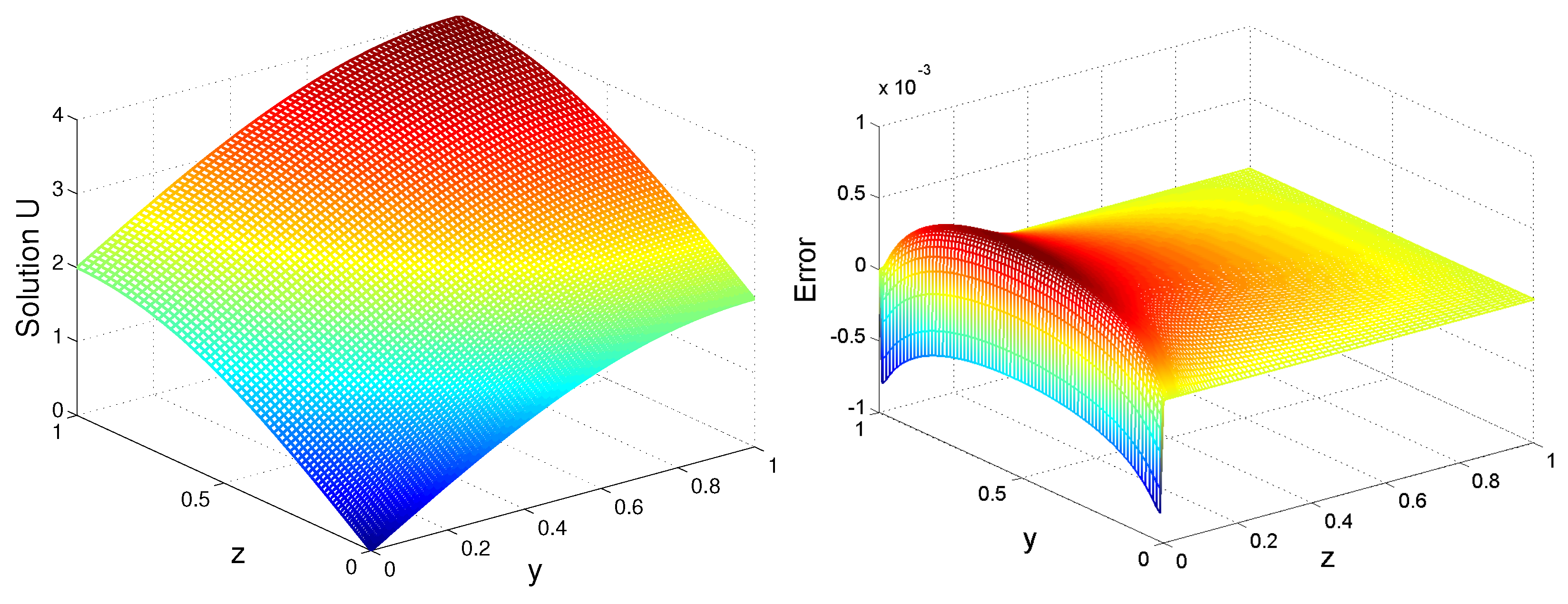
8. Numerical Experiments

In this section, we numerically study the temporal and spatial accuracy of the numerical schemes (32)–(34) and (40)–(45). We consider the case of less regular weak singular solution [49]

$$\left|\frac{{\partial }^{q}u}{\partial t^q}(·,t)\right|\le C(1+t^{\alpha -q}),q=0,1,2,\mathrm{for}\mathrm{all}(·,t)\in \overline{\mathsf{\Omega }}\times (0,T].$$

(46)

Meshes. Computations are performed on a fitted temporal mesh [49,51,56]

$$t_n=T{\left(\frac{n}{M}\right)}^m,m>1,n=0,1,\dots ,M.$$

(47)

We introduce the spatial mesh ${\overline{\omega }}_h$ with grid nodes, concentrated close to the degeneration boundaries

$$z_i=\left\{\begin{array}{ccc}{\displaystyle \frac{Z}{\nu }{\left(\frac{\nu i}{N}\right)}^2,}\hfill & {\displaystyle i=0,1,\dots ,\frac{N^{*}}{\nu }-1,}\hfill & \mathrm{if}\mathrm{increasing}\mathrm{order}\mathrm{of}i,\hfill \\ {\displaystyle \frac{Z}{\nu }-Z^{*}+\frac{Z}{\nu }{\left(\frac{N-\nu i}{N}\right)}^2,}\hfill & {\displaystyle i=\frac{N^{*}}{\nu },\frac{N^{*}}{\nu }+1,\dots ,N,}\hfill & \mathrm{if}\mathrm{increasing}\mathrm{order}\mathrm{of}i.\hfill \end{array}\right.$$

(48)

The parameters $N^{*}$, $\nu$ and $Z^{*}$ are determined as follows:

•$N^{*}=N$, $\nu =2$, $Z^{*}=0$, if $k(0,t)=k(Z,t)=0$;

•$N^{*}=N+1$, $\nu =1$, $Z^{*}=0$, if $k(0,t)=0$ and $k(Z,t)\ne 0$;

•$N^{*}=0$, $\nu =1$, $Z^{*}=Z$, if $k(0,t)\ne 0$ and $k(Z,t)=0$.

Error and convergence. Let

$$\begin{array}{ccc}& & \mathcal{E}=\mathcal{E}(M,N)=\underset{0\le i\le N}{max}\underset{0\le n\le M}{max}|u(z_i,t_{n+1})-U_i^{n+1}|\mathrm{for}1\mathrm{D}\mathrm{problem},\hfill \\ & & \mathcal{E}=\mathcal{E}(M,P,N)=\underset{0\le j\le P}{max}\underset{0\le i\le N}{max}\underset{0\le n\le M}{max}|u(y_j,z_i,t_{n+1})-U_{j,i}^{n+1}|\mathrm{for}2\mathrm{D}\mathrm{problem}.\hfill \end{array}$$

In view of (46) and the results in [49], we deduce that the solution $U^{n+1}$, computed by (32)–(34) or (40)–(45) on the graded temporal mesh (47) satisfies the estimate

$$\mathcal{E}\le \mathcal{C}(\delta P^{-2}+N^{-2}+T^{\alpha }{M}^{-min\{2-\alpha ,m\alpha \}}),$$

(49)

where $\mathcal{C}$ is a constant, $\delta =0$ for the 1D case, and $\delta =1$ for 2D case. Thus, as in [49], we choose

$$m=(2-\alpha )/\alpha ,$$

(50)

in order to achieve the optimal convergence in time $O\left({\tau }^{2-\alpha }\right)$.

The order of convergence is computed by

$$\begin{array}{ccc}& & {\mathcal{CR}}_{\tau }={log}_2\frac{\mathcal{E}(M,N)}{\mathcal{E}(2M,N)},{\mathcal{CR}}_h={log}_2\frac{{\mathcal{E}}_h(M,N)}{{\mathcal{E}}_h(M,2N)},\hfill \\ & & {\mathcal{E}}_h={\mathcal{E}}_h(M,N)=\underset{0\le j\le N}{max}\underset{0\le i\le N}{max}|u(y_j,z_i,T)-U_{j,i}^M|.\hfill \end{array}$$

Example 1 (1D problem: convergence).

We verify the order of convergence of the numerical scheme (32)–(34) for solving the advection–dispersion pollutant 1D problem in the domain $[0,1]\times [0,1]$ with a vertical diffusion coefficient and wind speed corresponding to (2) and (3)

$$k(z,t)=2t{z}^{{\beta }_1}{(1-z)}^{{\beta }_2},b(z,t)=3\mu +t{z}^{0.4},q(z,t)=-2zt,\mu =\{-1,1\},$$

${\beta }_1\ge 0$, ${\beta }_2\ge 0$, ${\beta }_1+{\beta }_2>1$. In the model (4)–(6), (17), written in divergent form (7), (17), we take $b(z,t)=-w(z,t)$ and set $f(z,t)$ such that $u(z,t)=(t^{\alpha }+t^{1+\alpha })sin(\pi z/2)$ to be the exact solution. Note that since $b(0,t)<0$ and $b(1,t)<0$ for $\mu =-1$, $t\in [0,T]$, in this case, we consider the Dirichlet boundary condition, in convention with the exact solution, at $z=0$. For $\mu =1$, we have $b(0,t)>0$ and $b(1,t)>0$. Therefore, Dirichlet boundary conditions at $z=Z$ must be imposed. In

Table 1. Errors and spatial convergence rate on uniform (UN) and nonuniform (NUM) spatial meshes, $\alpha =0.5$, Example 1.

	${\overline{\mathit{\omega }}}_{\mathit{h}}$	$({\mathit{\beta }}_1,{\mathit{\beta }}_2)$	$\mathit{\mu }$	$\mathit{N}=40$	$\mathit{N}=80$	$\mathit{N}=160$	$\mathit{N}=320$	$\mathit{N}=640$	$\mathit{N}=1280$
${\mathcal{E}}_h$	num	$(1,1.5)$	1	$6.953\times {10}^{-3}$	$1.977\times {10}^{-3}$	$5.294\times {10}^{-4}$	$1.372\times {10}^{-4}$	$3.496\times {10}^{-5}$	$8.825\times {10}^{-6}$
${\mathcal{CR}}_h$					1.814	1.901	1.947	1.973	1.986
${\mathcal{E}}_h$	um	$(1,1.5)$	1	$1.803\times {10}^{-2}$	$9.412\times {10}^{-3}$	$4.850\times {10}^{-3}$	$2.476\times {10}^{-3}$	$1.255\times {10}^{-3}$	$6.338\times {10}^{-4}$
${\mathcal{CR}}_h$					0.938	0.956	0.970	0.980	0.986
${\mathcal{E}}_h$	num	$(1,2)$	−1	$5.760\times {10}^{-3}$	$1.622\times {10}^{-3}$	$4.344\times {10}^{-4}$	$1.127\times {10}^{-4}$	$2.876\times {10}^{-5}$	$7.270\times {10}^{-6}$
${\mathcal{CR}}_h$					1.828	1.901	1.946	1.971	1.983
${\mathcal{E}}_h$	um	$(1,2)$	−1	$2.928\times {10}^{-2}$	$1.698\times {10}^{-2}$	$9.278\times {10}^{-3}$	$4.903\times {10}^{-3}$	$2.541\times {10}^{-3}$	$1.302\times {10}^{-3}$
${\mathcal{CR}}_h$					0.786	0.872	0.920	0.948	0.965
${\mathcal{E}}_h$	num	$(1.5,0)$	1	$6.149\times {10}^{-3}$	$2.180\times {10}^{-3}$	$7.649\times {10}^{-4}$	$2.640\times {10}^{-4}$	$9.033\times {10}^{-5}$	$2.821\times {10}^{-5}$
${\mathcal{CR}}_h$					1.496	1.511	1.535	1.547	1.679
${\mathcal{E}}_h$	um	$(1.5,0)$	1	$3.197\times {10}^{-2}$	$1.683\times {10}^{-2}$	$8.740\times {10}^{-3}$	$4.490\times {10}^{-3}$	$2.290\times {10}^{-3}$	$1.158\times {10}^{-3}$
${\mathcal{CR}}_h$					0.926	0.946	0.961	0.971	0.984

, we give the results from the computations on graded temporal mesh (47), (50) and both on uniform and nonuniform (48) meshes for different degeneration orders ${\beta }_1$, ${\beta }_2$ and fractional-order $\alpha =0.5$. The expected order of convergence on nonuniform spatial mesh is $O(M^{-(2-\alpha )}+N^{-2})$, taking into account (49). Therefore, we chose $M=N^{2/(2-\alpha )}$ for all runs. Obviously, the order of convergence in space is first on uniform mesh and close to second on the adapted spatial mesh (48).

Next, we test the temporal convergence. In

Table 2. Errors and temporal convergence rate, ${\beta }_1=1$, ${\beta }_2=2$, Example 1.

$\mathit{\alpha }$		$\mathit{M}=20$	$\mathit{M}=40$	$\mathit{M}=80$	$\mathit{M}=160$	$\mathit{M}=320$	$\mathit{M}=640$
0.25	$\mathcal{E}$	$4.204\times {10}^{-3}$	$1.310\times {10}^{-3}$	$3.994\times {10}^{-4}$	$1.204\times {10}^{-4}$	$3.606\times {10}^{-5}$	$1.076\times {10}^{-5}$
	${\mathcal{CR}}_{\tau }$		1.682	1.714	1.730	1.740	1.744
0.5	$\mathcal{E}$	$8.441\times {10}^{-3}$	$3.179\times {10}^{-3}$	$1.167\times {10}^{-3}$	$4.219\times {10}^{-4}$	$1.511\times {10}^{-4}$	$5.384\times {10}^{-5}$
	${\mathcal{CR}}_{\tau }$		1.409	1.446	1.468	1.481	1.489
0.85	$\mathcal{E}$	$2.069\times {10}^{-2}$	$1.037\times {10}^{-2}$	$5.050\times {10}^{-3}$	$2.368\times {10}^{-3}$	$1.098\times {10}^{-3}$	$5.039\times {10}^{-4}$
	${\mathcal{CR}}_{\tau }$		0.997	1.038	1.093	1.108	1.124

, we list the errors and orders of convergence of the solution for different values of $\alpha$ and ${\beta }_1=1$, ${\beta }_2=2$. The computations are performed on graded temporal mesh (47), (50) and uniform spatial mesh. In the previous tests (Table 1), we illustrated that the spatial order of convergence on uniform mesh is first. Therefore, we fix the number of the temporal grid nodes $N=M^{2-\alpha }$ in order to derive the convergence rate in time. The results in Table 2 show that the temporal convergence rate is $2-\alpha$.

Example 2 (1D problem: comparison).

The test example is (4)–(6), written in divergent form (7), (17), $z\in [0,5]$, $t\in [0,1]$ with $k(z,t)$ and $b(z,t)=-w(z,t)$, corresponding to (1) and (3), respectively

$$k(z,t)=2{(5-z)}^2,b(z,t)=-5+t{z}^{0.4},q(z,t)=-3z-t,$$

and $f(t,z)$ is determined such that $u(t,z)=(t^{\alpha }+t^{1+\alpha })e^{-z}$ to be the exact solution. For this numerical experiment, in view of the (8)–(12), we impose the Dirichlet boundary condition at $z=0$.

We will compare the efficiency of the numerical scheme (32)–(34) with upwind finite difference scheme, constructed following the boundary condition conception in Section 4:

$$\begin{array}{cc}\hfill & U_0^{n+1}=u(0,t_{n+1}),\hfill \\ \hfill & a_{n,n}{U}_i^{n+1}-\frac{k_{i+1/2}^{n+1}}{{\hslash }_i}{U}_{z,i}^{n+1}+\frac{k_{i-1/2}^{n+1}}{{\hslash }_i}{U}_{\overline{z},i}^{n+1}+{\left(b_i^{n+1}\right)}^{-}{U}_{\overline{z},i}^{n+1}-{\left(b_i^{n+1}\right)}^{+}{U}_{z,i}^{n+1}-q_i^{n+1}{U}_i^{n+1}\hfill \\ \hfill & =f_i^{n+1}+G_n{U}_i^n,i=1,2,\dots ,N-1,\hfill \\ \hfill & a_{n,n}{U}_N^{n+1}+\frac{k_{N-1/2}^{n+1}}{{\hslash }_N}{U}_{\overline{z},N}^{n+1}+{\left(b_N^{n+1}\right)}^{-}{U}_{\overline{z},N}^{n+1}-q_N^{n+1}{U}_N^{n+1}=f_N^{n+1}+G_n{U}_N^n,\hfill \end{array}$$

(51)

where $b^{+}=max\{b,0\}$, $b^{-}=max\{-b,0\}$. On uniform spatial mesh and temporal mesh (47), (50), both schemes (32)–(34) and (51) are first-order accurate in space, but the precision of (32)–(34) is much better.

We compute the solution on nonuniform spatial mesh (48), $N=320$ and graded temporal mesh, $M=1000$ for $\alpha =0.25$ in order to achieve a higher order of convergence in space. On Figure 1, we depict the error of the solution of (51) and (32)–(34) at the final time. The upwind scheme (51) fails in improving the accuracy on adapted spatial mesh. In contrast, the precision of the solution of the numerical discretization (32)–(34) is high since, as it is shown in Example 1, the order of convergence in space becomes second.

Example 3 (2D problem).

We verify the order of convergence of the numerical scheme (32)–(34). In the y-direction, we consider uniform mesh ${\tilde{\omega }}_h$ with step size $h^y$, while in the z-direction, we use fitted mesh (48). The temporal mesh is (47), (50).

We consider the following test examples

(𝖠) $k_z(z,t)$ is given by (2), $\mathrm{w}(z,t)$ is given by (3), $k_y=2\underset{{\overline{Q}}_T}{max}{k}_z$, $\mathrm{v}=1$, $q=-2xt$ [57];

(𝖡) ${\displaystyle k_z\left(z\right)=\frac{\kappa u_{*}L}{4.7}{\left(1-\frac{z}{Z}\right)}^2}$ as in (1), $k_y=2\underset{{\overline{Q}}_T}{max}{k}_z$, ${\displaystyle \mathrm{w}(z,t)=u_r\left(t\right){\left(\frac{z}{z_r}\right)}^{\gamma }}$, $\mathrm{v}=-2$ m/s, $q=0$ [1,7,11,13,17];

(𝖢) $y\to x$, $\mathrm{u}\to \mathrm{v}$, $k_z=z$, $k_x=3z$, $\mathrm{v}\left(z\right)=z^{0.5}$, $\mathrm{w}$ is given by (3), $q=-5$ [9,17,22].

For the convergence test, the computational domain in space is $[0,1]\times [0,1]$ and $T=1$. The meteorological input parameters are chosen as follows. In example (𝖠), $L=-8$, $\phi \left(t\right)=2t$, $k_y=15{\mathrm{m}}^2/\mathrm{s}$, $z_r=1$ m, $\tilde{u}=5$ m/s, $\delta =0.4$, $u_r\left(t\right)=t$, while for test (𝖡), we choose $L=4$, $u_{*}=2.5$ m/s, $u_r=1$, $\gamma =0.4$, $z_r=0.8$ m. In the experiment (𝖢), we replace the y variable with x in Equation (39) and obtain a crosswind-integrated pollutant problem at location $(x,z,t)\in [0,X]\times [0,Z]\times [0,T]$, where $k_x$ is the turbulent diffusion in the x-direction and $\mathrm{v}$ is the horizontal wind speed. For this example, we take $z_r=1$ m, $\tilde{v}=-3$ m/s, $u_r\left(t\right)=-2t$,

The right-hand side in (39) is determined such that $u(y,z,t)=(t^{\alpha }+t^{1+\alpha })(\sin (\pi z/2)+sin(\pi y/2))$ is the exact solution.

In

Table 3. Errors and spatial convergence rate, $\alpha =0.25$, Example 3.

𝖳𝖾𝗌𝗍		$\mathit{N}=10$	$\mathit{N}=20$	$\mathit{N}=40$	$\mathit{N}=80$	$\mathit{N}=160$	$\mathit{N}=320$
(𝖠)	${\mathcal{E}}_h$	$1.20\times {10}^{-2}$	$3.363\times {10}^{-2}$	$9.338\times {10}^{-3}$	$2.521\times {10}^{-3}$	$6.628\times {10}^{-4}$	$1.712\times {10}^{-4}$
	${\mathcal{CR}}_h$		1.838	1.848	1.889	1.927	1.953
(𝖡)	${\mathcal{E}}_h$	$2.439\times {10}^{-2}$	$7.842\times {10}^{-3}$	2.440$\times {10}^{-4}$	$7.302\times {10}^{-4}$	$2.037\times {10}^{-4}$	$4.653\times {10}^{-5}$
	${\mathcal{CR}}_h$		1.637	1.685	1.740	1.842	2.130
(𝖢)	${\mathcal{E}}_h$	1.917 $\times {10}^{-2}$	$7.683\times {10}^{-3}$	$2.592\times {10}^{-3}$	$7.999\times {10}^{-4}$	$2.334\times {10}^{-4}$	$6.549\times {10}^{-5}$
	${\mathcal{CR}}_h$		1.319	1.567	1.696	1.777	1.833

and

Table 4. Errors and spatial convergence rate, $\alpha =0.85$, Example 3.

𝖳𝖾𝗌𝗍		$\mathit{N}=10$	$\mathit{N}=20$	$\mathit{N}=40$	$\mathit{N}=80$	$\mathit{N}=160$	$\mathit{N}=320$
(𝖠)	${\mathcal{E}}_h$	$1.202\times {10}^{-1}$	$3.363\times {10}^{-2}$	$9.339\times {10}^{-3}$	$2.521\times {10}^{-3}$	$6.628\times {10}^{-4}$	$1.691\times {10}^{-4}$
	${\mathcal{CR}}_h$		1.838	1.848	1.889	1.928	1.971
(𝖡)	${\mathcal{E}}_h$	$2.247\times {10}^{-2}$	$7.327\times {10}^{-3}$	$2.311\times {10}^{-3}$	$6.980\times {10}^{-4}$	$2.015\times {10}^{-4}$	$5.691\times {10}^{-5}$
	${\mathcal{CR}}_h$		1.616	1.665	1.727	1.792	1.824
(𝖢)	${\mathcal{E}}_h$	$1.968\times {10}^{-2}$	$7.766\times {10}^{-3}$	$2.605\times {10}^{-3}$	$8.018\times {10}^{-4}$	$2.336\times {10}^{-4}$	$6.449\times {10}^{-5}$
	${\mathcal{CR}}_h$		1.341	1.576	1.700	1.779	1.857

, we give the computational results. All runs are performed for $P=N$, $\alpha =0.25$ (Table 3), $\alpha =0.85$ (Table 4) and $M=N^{2/(2-\alpha )}$ (in view of (49), (50)). We observe that for all test problems, the spatial order of convergence is close to second.

On Figure 2 and Figure 3, we plot the numerical solution and error at the final time for 𝖡, $\alpha =0.25$ and 𝖢, $\alpha =0.85$. The numbers of mesh grid nodes are $P=N=80$, $M=N^{2/(2-\alpha )}$.

9. Conclusions

Model-turbulent degenerate subdiffusion equations of contaminant dispersion in the planetary boundary layer are considered. The degeneration behavior of the coefficients in the equation follows models with power–law function diffusitivity profiles and wind velocity profiles of a similar character. Well posedness and a priori estimates for the solutions are obtained. Additionally, the maximum principle is proved and used for studying properties of the solution.

We construct an unconditional positivity-preserving numerical scheme that successfully overcomes space degeneration. The discretization is realized on space- and time-adaptive meshes so as to obtain optimal accuracy—second order in space and $2-\alpha$ in time.

References

1. Arya, S.P. Air Pollution Meteorology and Disperision; Oxford University Press: New York, NY, USA, 1999; 310p. [Google Scholar]
2. Blackadar, A.K. Turbulence and Diffusion in the Atmosphere: Lectures in Environmental Science; Springer: Berlin, Germany, 1997; 185p. [Google Scholar]
3. Goulart, A.G.O.; Lazo, M.J.; Suarez, J.M.S.; Moreira, D.M. Fractional derivative models for atmospheric dispersion of pollutants. Phys. A Stat. Mech. Its Appl. 2017, 477, 9–19. [Google Scholar] [CrossRef]
4. Marchuk, G.I. Mathematical modelling in environmental problems. Stud. Math. Its Appl. 1986, 16, 1986. [Google Scholar]
5. Goulart, A.G.O.; Lazo, M.J.; Suarez, J.M.S. A new parameterization for the concentration flux using the fractional calculus to model the dispersion of contaminants in the Planetary Boundary Layer. Phys. A Stat. Mech. Its Appl. 2019, 518, 38–49. [Google Scholar] [CrossRef]
6. Moreira, D.; Moret, M. A new direction in the atmospheric pollutant dispersion inside the planetary boundary layer. J. Appl. Meteorol. Climatol. 2018, 57, 185–192. [Google Scholar] [CrossRef]
7. Moreira, D.M.; Santos, C.A.G. New approach to handle gas-particle transformation in air pollution modelling using fractional derivatives. Atmos. Pollut. Res. 2019, 10, 1577–1587. [Google Scholar] [CrossRef]
8. Sylvain, T.T.A.; Patrice, E.A.; Marie, E.E.J.; Pierrea, O.A.; Huberta, B.-B.G. A three-dimensional fractional solution for air contaminants dispersal in the planetary boundary layer. Heliyon 2021, 7, e07005. [Google Scholar]
9. Sylvain, T.T.A.; Patrice, E.A.; Marie, E.E.J.; Pierre, O.A.; Hubert, B.B.G. Analytical solution of the steady-state atmospheric fractional diffusion equation in a finite domain. Pramana-J. Phys. 2021, 95, 1. [Google Scholar] [CrossRef]
10. Golant, E.I. Conjugate families of difference schemes for equations of parabolic type with lowest terms. Zh. Vychisl. Mat. Mat. Fiz. 1978, 18, 1162–1169. [Google Scholar] [CrossRef]
11. Hosseini, B.; Stockie, J.M. Estimating airborne particulate emissions using a finite-volume forward solver coupled with a Bayesian inversion approach. Comput. Fluids 2017, 154, 27–43. [Google Scholar] [CrossRef]
12. Moreira, D.M.; Rizza, U.; Vilhena, M.T.; Goulart, A. Semi-analytical model for pollution dispersion in the planetary boundary layer. Atmos. Environ. 2005, 39, 2673–2681. [Google Scholar] [CrossRef]
13. Troen, I.B.; Mahrt, L. A simple model of the atmospheric boundary layer; sensitivity to surface evaporation. Boundary-Layer Meteorol. 1986, 37, 129–148. [Google Scholar] [CrossRef]
14. Vulkov, L.G. Well-posedness for initial value problems of atmospheric flow models with degenerate vertical diffusion. AIP Conf. Proc. 2022, 2505, 030003. [Google Scholar]
15. Albani, R.A.S.; Albani, V.V.L.; Neto, A.J.S. Genetic algorithm optimization applied to source estimation in the atmosphere. In Proceedings of the 18th Brazilian Congress of Thermal Sciences and Engineering, Online, 16–20 November 2020. [Google Scholar] [CrossRef]
16. Albani, R.A.S.; Duda, F.P.; Pimentel, L.C.G. On the modeling of atmospheric pollutant dispersion during a diurnal cycle: A finite element study. Atmos. Environ. 2015, 118, 19–27. [Google Scholar] [CrossRef]
17. Stockie, J.M. The mathematics of atmospheric dispersion modeling. SIAM Rev. 2011, 53, 349–372. [Google Scholar] [CrossRef]
18. Kandilarov, J.; Vulkov, L. Determination of concentration source in a fractional derivative model of atmospheric pollution. AIP Conf. Proc. 2021, 2333, 090014. [Google Scholar]
19. Caputo, M. Vibrations of infinite viscoelastic layer with a dissipative memory. J. Acoust. Soc. Am. 1974, 56, 897–904. [Google Scholar] [CrossRef]
20. Klibas, A.A.; Srivastava, H.M.; Trujillo, J.J. Theory and Applications of Fractional Differential Equations; Elsevier: Amsterdam, The Netherlands, 2006; p. 540. [Google Scholar]
21. Podlubny, I. Fractional Differential Equations; Academic Theory and Applications of Fractional Differential Equations; Elsevier: Amsterdam, The Netherlands, 1998. [Google Scholar]
22. Arora, U.; Gakkhar, S.; Gupta, R.S. Removal model suitable for air pollutants from an elevated source. Appl. Math. Model. 1991, 15, 386–389. [Google Scholar] [CrossRef]
23. Bhaskar, C.; Lakshminarayanachari, K. Numerical model for primary and secondary air pollutants emitted from an area and point source in an urban area with chemical reaction and removal mechanisms. Mater. Today 2021, 37, 2961–2967. [Google Scholar] [CrossRef]
24. Blottner, F.G.; Lopez, A.R. Determination of Solution Accuracy of Numerical Scheme as Part Code and Calculation Verification; Sandia National Laboratories: Albuquerque, NM, USA; Livermore, CA, USA, 1998; 77p.
25. Chernogorova, T.P.; Koleva, M.N.; Vulkov, L.G. Exponential finite difference scheme for transport equations with discontinuous coefficients in porous media. Appl. Math. Comput. 2021, 392, 125691. [Google Scholar]
26. Dang, Q.A.; Ehrhardt, M. Adequate numerical solution of air pollution problems by positive difference schemes on unbounded domains. Math. Comput. Model. 2006, 44, 834–856. [Google Scholar] [CrossRef]
27. Dang, Q.A.; Ehrhardt, M.; Tran, G.L.; Le, D. On the numerical solution of some problems ofenvironmental pollution. In Air Pollution Research Advances; Bodine, C.G., Ed.; Nova Science Publishers, Inc.: Hauppauge, NY, USA, 2007. [Google Scholar]
28. Koleva, M.N.; Vulkov, L.G. Positivity-preserving finite volume difference schemes for atmospheric dispersion models with degenerate vertical diffusion. Comp. Appl. Math. 2022, 41, 406. [Google Scholar] [CrossRef]
29. Monin, A.S.; Obukhov, A.M. Basic laws of turbulent mixing in the surface layer of the atmosphere. Tr. Akad. Nauk. SSSR Geophiz. Inst. 1954, 24, 163–187. [Google Scholar]
30. Dimov, I.T.; Kandilarov, J.D.; Vulkov, L.G. Numerical Identification of the Time Dependent Vertical Diffusion Coefficient in a Model of Air Pollution. In Advanced Computing in Industrial Mathematics; Studies in Computational Intelligence; Georgiev, I., Kostadinov, H., Lilkova, E., Eds.; Springer: Cham, Switzerland, 2021; Volume 961. [Google Scholar]
31. Koleva, M.N. Numerical method for space degenerate fractional derivative problems of atmospheric pollution. AIP Conf. Proc. 2022, 2505, 080024. [Google Scholar]
32. Fazio, R.; Jannelli, A.; Agreste, S. A Finite Difference Method on Non-Uniform Meshes for Time-Fractional Advection–Diffusion Equations with a Source Term. Appl. Sci. 2018, 8, 960. [Google Scholar] [CrossRef]
33. Shiri, B.; Baleanu, D. A general fractional pollution model for lakes. Commun. Appl. Math. Comput. 2022, 4, 1105–1130. [Google Scholar]
34. Mahsud, Y.; Shah, N.A.; Vieru, D. Influence of time-fractional derivatives on the boundary layer flow of Maxwell fluids. Chin. J. Phys. 2017, 55, 1340–1351. [Google Scholar] [CrossRef]
35. Van Bockstal, K. Uniqueness for inverse source problems of determining a space-dependent source in time-fractional equations with non-smooth solutions. Fractal Fract. 2021, 5, 169. [Google Scholar] [CrossRef]
36. Koleva, M.N.; Vulkov, L.G. Numerical identification of external boundary conditions for time fractional parabolic equations on disjoint domains. Fractal Fract. 2023, 7, 326. [Google Scholar] [CrossRef]
37. Long, L.D.; Zhou, Y.; Thanh Binh, T.; Can, N. A mollification regularization method for the inverse source problem for a time fractional diffusion equation. Mathematics 2019, 7, 1048. [Google Scholar] [CrossRef]
38. Ozbilge, E.; Kanca, F.; Ozbilge, E. Inverse problem for a time fractional parabolic equation with nonlocal boundary conditions. Mathematics 2022, 10, 1479. [Google Scholar] [CrossRef]
39. Yang, F.; Gao, Y.-X.; Li, D.-G.; Li, X.-X. Identification of the initial value for a time-fractional diffusion equation. Symmetry 2022, 14, 2569. [Google Scholar] [CrossRef]
40. Abbaszadeh, M.; Dehghan, M. Numerical and analytical investigations for solving the inverse tempered fractional diffusion equation via interpolating element-free Galerkin (IEFG) method. J. Therm. Anal. Calorim. 2021, 143, 1917–1933. [Google Scholar] [CrossRef]
41. Kinash, N.; Janno, J. An inverse problem for a generalized fractional derivative with an application in reconstruction of time- and space-dependent sources in fractional diffusion and wave equations. Mathematics 2019, 7, 1138. [Google Scholar] [CrossRef]
42. Kinash, N.; Janno, J. Inverse problems for a generalized subdiffusion equation with final overdetermination. Math. Model. Anal. 2019, 24, 236–262. [Google Scholar]
43. Koleva, M.N.; Vulkov, L.G. Analytical and computational analysis of space degenerate time fractional parabolic model of atmospheric dispersion of pollutants. AIP Conf. Proc. 2023; accepted. [Google Scholar]
44. Alikhanov, A.A. A priori estimates for solutions of boundary value problems for fractional-order equations. Differ. Equ. 2010, 46, 660–666. [Google Scholar] [CrossRef]
45. Luchko, Y. Some uniqueness and existence results for the initial-boundary-value problems for the generalized time-fractional diffusion equation. Comput. Math. Appl. 2010, 59, 1766–1772. [Google Scholar] [CrossRef]
46. Brunner, H.; Han, H.; Yin, D. The Mmaximum principle for time-fractional diffusion equations and its application. Numer. Funct. Optim. 2015, 36, 1307–1321. [Google Scholar] [CrossRef]
47. Popov, I.V. On monotonic differential schemes. Matem. Mod. 2019, 31, 21–43. [Google Scholar]
48. Samarskii, A.A. Theory of Finite Difference Schemes; Marcel Decker: New York, NY, USA, 2001; 786p. [Google Scholar]
49. Stynes, M.; O’Riordan, E.; Gracia, J.L. Error analysis of a finite difference method on graded meshes for a time-fractional diffusion equation. SIAM J. Numer. Anal. 2017, 55, 1057–1079. [Google Scholar] [CrossRef]
50. Zhanga, Y.; Sun, Z.; Liao, H. Finite difference methods for the time fractional diffusion equation on non-uniform meshes. J. Comput. Phys. 2014, 265, 195–210. [Google Scholar] [CrossRef]
51. Chen, H.; Stynes, M. Error analysis of a second-order method on fitted meshes for a time-fractional diffusion problem. J. Sci. Comput. 2019, 79, 624–647. [Google Scholar] [CrossRef]
52. Alikhanov, A.A. A new difference scheme for the time fractional diffusion equation. J. Comput. Phys. 2015, 280, 424–438. [Google Scholar] [CrossRef]
53. Zhou, B.; Chen, X.; Li, D. Nonuniform Alikhanov Linearized Galerkin Finite Element Methods for Nonlinear Time-Fractional Parabolic Equations. J. Sci. Comput. 2020, 85, 39. [Google Scholar] [CrossRef]
54. Faragó, I.; Horváth, R.; Korotov, S. Discrete maximum principle for linear parabolic problems solved on hybrid meshes. Appl. Numer. Math. 2005, 53, 249–264. [Google Scholar] [CrossRef]
55. Ulke, A.G. New turbulent parameterization for a dispersion model in the atmospheric boundary layer. Atmos. Environ. 2000, 34, 1029–1042. [Google Scholar] [CrossRef]
56. Chen, H.; Stynes, M. A high order method on graded meshes for a time-fractional diffusion problem. In Finite Difference Methods. Theory and Applications; Lecture Notes in Computer, Science; Dimov, I., Farago, I., Vulkov, M.L., Eds.; Springer: Cham, Switzerland, 2019; p. 11386. [Google Scholar]
57. Tangerman, G. Numerical Simulations of Air Pollutant Dispersion in a Stratified Planetary Boundary Layer. Atmos. Environ. 1978, 12, 1365–1369. [Google Scholar] [CrossRef]
Figure 1. Errors vs. the number of spatial grid nodes for (51) (left) and (32)–(34) (right), α = 0.25 , graded space–time meshes, N = 320 , M = 1000 , Example 2.
Mathematics 11 02040 g001
Figure 2. Solution (left) and error (right) vs. the number of spatial grid nodes for (40)–(45), test (𝖡), α = 0.25 , N = P = 80 , Example 3.
Mathematics 11 02040 g002
Figure 3. Solution (left) and error (right) vs. the number of spatial grid nodes for (40)–(45), test (𝖢), α = 0.85 , N = P = 80 , Example 3.
Mathematics 11 02040 g003