1. Introduction
On-demand home delivery services are quickly absorbing the commercial operations of sellers of stationery products and grocery, food, personal care, and pharmaceutical products. Evidently, the coronavirus outbreak and the subsequent nationwide lockdown played a part. Nowadays, most individuals prefer having things delivered to their homes rather than carrying the purchased item from the store.
Motivation: In the month of June 2022, one of the authors went to a Vasanth & Co. store to buy a refrigerator at Mylapore in Chennai, Tamil Nadu, India. He looked at how the shop worked and saw the following. On that day, the store was very busy selling refrigerators to new customers. The shop had only two servers. One server was always connected to the system so that the refrigerator could be sold. At the end of the service, the server asked the customer if they wanted to have it delivered to their door or if they wanted to carry it themselves. Due to some practical issues, the customer chose a home delivery service. After seeing how the shop worked, we made the stochastic model with a door-to-door delivery facility.
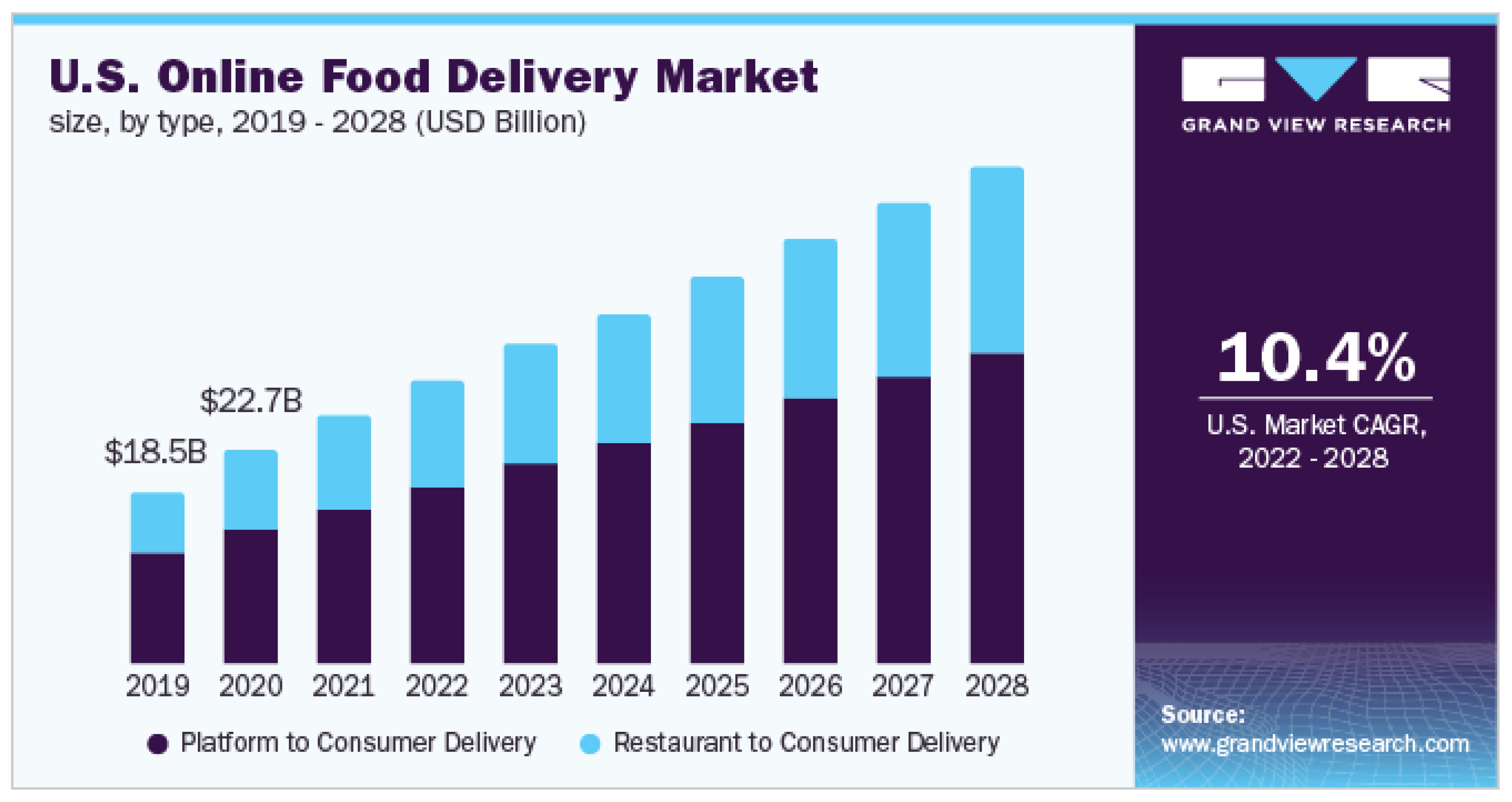
In 2021, the worth of the worldwide online food delivery market was USD 189.70 billion, and it is predicted to expand at a compound annual growth rate (CAGR) of 10.8% from 2022 to 2028, as shown in
Figure 1. The driving force behind this growth is the increasing number of smartphone and internet users, boosting the demand for online food delivery platforms.
Due to the spread of the COVID-19 pandemic, there has been a significant increase in the demand for food and grocery delivery services due to lockdowns and social-distancing measures. As a result, there has been a proliferation of delivery services worldwide, including in markets, farms, and online stores. The pandemic has brought to light the importance of delivery services in meeting customer needs and has also led to the emergence of hyperlocal delivery strategies.
The application of home delivery services in real-life businesses encourages us to conduct research in such areas. The author’s visiting experience in the retail shop, the data illustrated in
Figure 1, and customer requirements during the pandemic period inspire us to bring such stochastic modeling.
The rest of the paper is organized as follows. The literature review is provided in
Section 2. In
Section 3, a comprehensive explanation is provided. The development of transition matrices and solutions to stationary probability vectors is analyzed in
Section 4. In
Section 5, the system performance metrics are discussed. In
Section 6, numerical results and discussions are presented. In
Section 7, the conclusions and future directions are discussed.
2. Literature Review
In today’s society, there are two different types of businesses that provide service to their customers: one is a product-based business (home appliances, groceries, and so on) and the other is a non-product-based business (office work, bank work, ticket services, and so on). These types of businesses are explored by the queuing-inventory system (QIS) and the queuing system (QS). According to the queuing-inventory literature, Melikov and Molchanov [
1] and Sigman and Simchi-Levi [
2] introduced the service facility to improve customer satisfaction. Many authors have discussed the positive service time in the inventory system for the last two decades. For more details about the positive service time, the readers can refer to Krishnamoorthy et al. [
3]. They presented a survey of authors who have contributed to the inventory system with positive service time.
Krishnamoorthy et al. [
4] analyzed a batch arrival and service process in a QIS. At the end of service completion, there will be a unit item from the inventory depleted, irrespective of batch size. If the server is on vacation, he or she is busy preparing the items up to the predetermined size
L for future service. Suppose the preparation service is over and the vacation period is not yet completed; then, he or she will become idle there. If there must be
N customers available in the system at the end of the vacation, he or she begins service. They also computed the processing time in a vacation cycle and the idle time in a vacation cycle. Yuying Zhang et al. [
5] discussed a QIS with server vacation. When the server is off due to vacation, they assume that an arriving new customer may be lost and a waiting customer in the queue may get impatient. Nithya et al. [
6] looked into a retrial QIS with server multiple vacations. In addition, they studied this vacation facility with a state-dependent arrival admission.
Yuying Zhang et al. [
7] studied a multiple server vacation, randomized order policy, and lost sales in the QIS. Sugapriya et al. [
8] analyzed a multiple server vacation in a QIS. They assumed that an input to the system is dependent on the current inventory level. The server takes another vacation if he returns from vacation and finds that there is no positive inventory. Furthermore, they presented a comparative result for stock dependency and non-stock dependency and obtained an efficient output for the earlier case. Recently, Linhong Li et al. [
9] discussed a stochastic QIS with multiple vacations and batch demands. That is, an arriving customer takes a batch of items after the completion of the service.
However, during the vacation period of a server, his/her vacation offer is abruptly interrupted due to the system requirement. This interruption is called a vacation interruption. Manikandan et al. [
10] worked in an inventory system with a working vacation. In this type, the server is allowed to work at a slower rate. Supposing that he finds at least one customer in the system at the end of a vacation period, he comes back to normal mode. Rajadurai et al. [
11] discussed the vacation interruption of the server in the unreliable G-queue. Due to the positive queue in the orbit, the server’s working vacation period is interrupted. Vijayashree et al. [
12] considered two types of vacations: one with a shorter duration and another with a longer duration. They assumed that vacation interruption is allowed only when the server is on a shorter vacation period.
As per the customers’ requirements, many companies have started home delivery services in the last two decades. Nowadays, it is an essential service facility that is mostly expected by the customer. Initially, home delivery (door delivery) was started by postal services and courier services. On this occasion, the delivery person took all the letters and started the delivery service one by one. Consequently, this service facility was extended to the parcel service. Gradually, milk and newspapers were delivered to the door by the local organizers. Following this, some local supermarkets, home appliance stores, and grocery stores offered door-to-door delivery to their customers.
The home delivery service was initiated in the queuing system for parcel delivery services (PDSs) from the courier office to the customer’s home. Hideyama et al. [
13] executed PDS by the parcel lockers. They argued that it would reduce the number of re-delivery procedures because at the time of delivery of the parcel, the customer may not be available in the home. In this situation, a locker facility would be much more helpful to deliver the parcels. It also reduces the extra transportation costs. The PDS also discussed using the parcel lockers in [
14]. Schnieder et al. [
15] discussed a collection of parcel deliveries and delivery points in their article and compared them with the home delivery results.
Jafer Heydari and Alireza Bakhshi [
16] discussed two types of contracts between an e-retailer and a third-party company to provide a home delivery service to the customer. They found an optimal contract policyholder for such a delivery facility. The deliveries of household goods at the door-to-door service facilities are discussed by Rosa Arroyo López and José Vicente Colomer Ferrándiz [
17].
The impact of planning and policies for home delivery services was discussed by Rosário Macário [
18]. Ana Peláez Bejarano et al. [
19] applied the home delivery service in a hospital pharmacy department during the COVID-19 pandemic. Briony Shaw et al. [
20] considered the idea of transitioning to hospitals in the home using home delivery. Snežana Tadić and Miloš Veljović [
21] described the advantages, disadvantages, interdependence, and applicability of different delivery models in changing circumstances. Christian Truden et al. [
22] provided a comprehensive computational study comparing several algorithmic strategies, combining heuristics utilizing local search operations and mixed-integer linear programs, and tackling the booking process for grocery home delivery services. Unnikrishnan and Figliozzi [
23] discussed the home delivery purchases and expenditures on the impact of the COVID-19 pandemic. Yang Liu and Sen Li [
24] presented an economic analysis for home delivery platforms with two types of interdependent markets: (1) the food delivery market and (2) the ride-sourcing market. Pinyi Yao et al. [
25] attempted to compare the differences between to-shop and to-home consumers for online-to-offline commerce. Vienna Klein and Claudius Steinhardt [
26] addressed the substantial operational challenges by combining a demand-management approach with an online tour-planning approach for same-day delivery. Yoon-Joo Park [
27] analyzed consumer preferences with regard to delivery services with different delivery times and packaging types, targeting South Korea’s online grocery markets.
Research Gap: So far, we have learned about the home delivery process in many ways, but it has not been studied in the stochastic queuing inventory approach yet. Thus, we consider the following assumptions as a research gap:
- (a)
In the domain of SQIM, there have been no papers published with a positive service time for home delivery service.
- (b)
Even though some authors discussed home delivery services other than SQIM, the discussion about the delivery server (person) is not analyzed.
- (c)
The vacation period of the delivery server and his vacation interruption due to the threshold level has not been analyzed.
Proposal of the Model: In response to the identified research gap, we integrated the home delivery service capability within the QIS domain. We utilize the delivery server (the delivery person) to deliver the merchandise to the customer’s door. The consumer may choose the door-to-door delivery option at the conclusion of the service. The system administrator extends a vacation offer to the server, which may be accepted up to a predetermined threshold level. The delivery server is permitted to take a vacation, but if the number of home delivery items surpasses a certain threshold, the vacation must be cut short. The replenishment of an item is believed to be part of the ordering policy for (). Additionally, perishable assumptions are also added.
3. Model Description
The stochastic queuing-inventory system (SQIS) considers the home delivery (door-to-door) service facility for consumers with self and mandatory interruptions during vacations. The SQIS stores the fresh inventory for sales of maximum size S and purchased inventories for home delivery of maximum size N in distinct storage spaces. The customer enters the system in order to purchase a single item. A customer’s arrival follows a Poisson process with parameter .
The system assigns Server-1 to handle sales service for the fresh product and Server-2 to handle door-to-door delivery service for the sold product. Server-1 is a stationary server that is always connected to the system. Server-2 is referred to as a delivery server because he must travel to provide a door-to-door delivery service. When Server-1 is free, and a number of items for sale have positive stock, an arriving customer receives rapid service. Otherwise, they must wait in the designated waiting room of size M. If the waiting area is already full, a new customer who just arrived is seen as lost. Server-1 must perform the sales service to the customer and completes the service process with a rate of whenever both are positive. Otherwise, he remains idle. The service time of Server-1 follows an exponential distribution. Every customer has the Bernoulli option to accept the home delivery service. After the service completion, the customer either leaves the system with a purchased product with probability , or hands over the purchased product for home delivery with probability , where and leaves the system without a purchased product.
Server-2 receives the vacation offer only if the number of home delivery products ordered does not exceed the n threshold level. If the number of home delivery items goes over the n threshold, the vacation offer must be withdrawn right away. Thus, the vacation is interrupted when the number of home delivery items reaches . At the epoch of the last door delivery service completion, he returns to the system and checks the currently available items for home delivery.
If it is less than , he either goes on vacation with a probability of or continues the home delivery service for the currently available home delivery stocks with a probability of , where . Each home delivery item is delivered to the customer at a rate of . The service time of Server-2 is exponentially distributed. The time between returning to the system of Server-2 at the last service completion epoch of the previously taken items for door delivery and picking up the currently received items for door delivery again and starting delivery service of the first product is negligible.
If there are no home delivery items available for door delivery, Server-2 remains on vacation. When the last service completion epoch occurs, at which Server-2 finds that there is one item available for door delivery, he either picks up and starts door delivery of the corresponding product with probability or goes on vacation with probability . Suppose he finds that there are 2 items available for door delivery; he again picks up the 2 items and starts the door delivery service one by one with probability or goes on vacation with probability . If the first item is delivered, then he starts a door-to-door delivery service for the second item to the corresponding customer. Again, after this service completion, if he finds that there are 3 items available for door delivery, he picks up the 3 items and starts door delivery of the first product with probability or goes on vacation with probability . If the first item of this turn is delivered, then he starts the door-to-door delivery of the second product, and after its completion, he goes to deliver the last one. In general, this vacation option and door delivery service process for Server-2 continue up to .
During the vacation period of Server-2, if he knows there are k items for home delivery, where , he may terminate his vacation by himself with a parameter . The process of switching from vacation to a busy period on Server-2 is called self vacation interruption. The time between an epoch, when Server-2 begins a vacation, and an epoch when Server-2 interrupts his vacation voluntarily, follows an exponential distribution. However, whether Server-2 is on vacation or at the last service completion epoch of the home delivery service, he is not permitted to take a vacation if the current number of home delivery items exceeds n. Such a vacation termination process is called a compulsory vacation interruption. Suppose , the home delivery service process is to be continued without an optional vacation. Server-2 takes k items and begins delivery service with the first item and works its way up to the kth item one by one.
Inventory in the first storage space can be defective at any time. The lifetime of a selling item is assumed to be exponentially distributed with an intensity rate
. It is to be noted that the product handed over for home delivery will not perish. If the number of items to be sold reaches the reorder point
s, an immediate reorder of
Q items is to be triggered. This ordering principle is called the
ordering principle. The time interval between two consecutive reorders is assumed to be exponentially distributed with a rate of
. The proposed model’s graphical sketch is given in
Figure 2.
4. Analysis of the Model
In this section, we discuss the random variables, transition matrices, and solutions to the stationary probability vector.
4.1. Assumptions of the Random Process
As we described in the model explanations in the previous section, first we shall define the random variables. Let
represent the number of items in the first storage space at time
t. Then
represents the number of customers in the waiting hall at time
t. Next,
represents the number of purchased items in the second storage space for home delivery at time
t. Finally,
represents the server status at time
t where
is the sum of the first
x natural number, that is,
For convenience, we use the notation
to denote the exact position of both servers, where
denotes that Server-1 is in an idle period,
denotes that Server-1 is in a busy period,
i represents the number of home delivery products that have to be taken by Server-2 at time
t, and
j indicates which home delivery product is currently being serviced to the customer (
and
). The status of both servers is represented by
Here, the random variables , where , are said to be continuous-time random variables. Hence, the collection of random variables indexed with time t, forms a four-dimensional stochastic process.
4.2. Construction of the State Space
According to the model assumptions and the defined random variables, we shall construct the state space of the model as follows:
Therefore, the state space is countably finite. The dimension of the state space is . Thus, the collection of continuous-time random variables has the discrete state space. Hence, the is said to be a continuous-time Markov chain (CTMC).
4.3. Construction of the Infinitesimal Generator Matrix
The CTMC
has the infinitesimal generator matrix
A, and it is formed as follows:
where the matrix
C represents the transitions of the reordering process of the CTMC and it contains a
block of the
-matrix along the diagonal of
C. Each
block consists of a
sub-matrix
and a
sub-matrix
along the diagonal, where
and
:
Now, we shall see the block matrix,
,
. It consists of the transitions between the perishable rate and service rate of Server-1. It has
sub-block matrix
and
M sub-block matrix
. The matrix
holds the transition of perishable rate with dimension
For
where
The
matrix represents the rate of service completion for a customer in the waiting hall. At the end of each service, a customer leaves the system with or without an item based on the Bernoulli schedule. In the latter case, the customer requires a home delivery service:
Here, the
and
matrices hold the same transition but in a different dimensions, say
and
respectively. Supposing the second storage space is full, a customer has no choice but to opt for a home delivery service. In this situation, he leaves the system with an item that is certain. It is represented in
. Similarly, the matrices
and
represent the same transition at which an item is added for home delivery service but of a different dimension, say
and
, respectively. Though the matrix
does the same as
, it is differed by its size of
, where
Furthermore, the matrix
represents the compulsory interruption of Server-2’s vacation period:
The block matrix
represents the diagonals of the generator matrix
A for
It consists of a
sub-matrix along the super diagonal. It holds the transition rate of arriving customers in the waiting hall:
where
The matrix
represents the general diagonal block structure. It completely describes a home delivery service process, the self-vacation interruption of Server-2, and diagonal elements. For
First, we shall explore the
matrix. It represents that Server-2 takes the items for home delivery service and begins service on the 1st item. For
, take
if either
or
and take
if
The matrix
represents a self-interruption of Server-2’s vacation when he finds
number of items,
:
The matrix
denotes that during the last service completion epoch, Server-2 decided to continue his home delivery service by taking the newly available home delivery items and starting service one by one. For
and
If
, Server-2 is not allowed to go on vacation. So, he must take all the available items for home delivery and start the delivery services:
For
and
The matrix
represents the diagonal matrix when both inventories are zero, where
:
The matrix
represents the diagonal matrix when
is zero,
and
:
The matrix
represents the diagonal matrix when
,
and
:
The matrices
and
denote that Server-2 goes on vacation transitions at the last service completion epoch. For
,
For
where
,
and
The matrix
represents the diagonal matrix when
and
:
The matrix
represents the diagonal matrix when
,
and
:
The matrix
represents the diagonal matrix when
,
and
:
where
and
where
,
and
The matrix
represents the diagonal matrix when
,
is empty, and
:
The matrix
represents the diagonal matrix when
,
and
:
The matrix
represents the diagonal matrix when
,
and
:
where
and
where
,
and
4.4. Solution of Stationary Probability Vector
Let denote the steady state probability vector of the system, and the probability vector represents the current inventory level of the system at time t.
4.5. Representation of Partition of Stationary Probability Vector
The partition of the probability vector
is given as follows:
4.6. Computation of Stationary Probability Vector
The stationary probability vector
is determined by setting
and
The relation
leads to the following system of equations:
The matrix equation
produces the
system of homogeneous linear equations. Now, solving the system of equations recursively, except the equation when
, we obtain all the
in terms of
where
. That is,
where
Here, the matrices
and
are defined as follows:
Computation of the Probability Vector
In the matrix equation
, consider the equation when
and substitute
and
in
Finally, solving the two equations
and
simultaneously, we obtain the value of the probability vector
5. Evaluation of Expected System Performance Measures
In this section, we shall construct the expected cost function in terms of S and s with the help of some important system characteristics of the model. In particular, the performance of the delivery server, the expected self-vacation interruption rate, the compulsory-vacation interruption rate, the number of products delivered at the customers’ homes, etc., are to be computed:
Expected inventory level (EIL): represents the EIL in the system at time
t,
Expected reorder rate (ERR): represents the ERR in the system at time
t,
Expected perishable rate (EPR): represents the EPR in the system at time
t,
Expected number of customers in the waiting hall (ECWH): represents the ECWH in the system at time
t,
Expected number of home delivery products (EHDP): represents the EHDP in the system at time
t,
Expected vacation interruption rate of Server-2 (EVI2): represents the EVI2 in the system at time
t,
- (a)
Expected self-vacation interruption rate of Server-2 (ESVI2): represents the ESVI2 in the system at time
t,
- (b)
Expected compulsory vacation interruption of server 2 (ECVI2) by the system: represents the (ECVI2) in the system at time
t,
Expected customer loss rate of the system(ECL): represents the ECL in the system at time
t,
Probability that Server-2 is on vacation (P(Server-2 is on vacation)): Probability that Server-1 is busy:
Expected Cost Analysis
The expected total cost value
of the system is determined by
where
and
denote the holding cost for the per-unit item in the inventory and the purchased product for home delivery at time
t, respectively. Then,
represents a set-up cost per order,
denotes a perishable cost per item, and
refers to the waiting cost per customer at time
t. The cost
represents a customer loss cost per customer.
Remark 1. In the proposed CTMC, the following limitations are encountered:
- 1.
When assuming , this model becomes an ordinary category.
- 2.
Assuming , all the customers compulsorily opt for the home delivery service.
- 3.
When assuming , Server-2 will not go on vacation unless is zero.
- 4.
When assuming , self vacation interruption of Server-2 is not allowed. The server will have a compulsory vacation interruption only.
6. Numerical Results and Discussions
In the proposed model, the numerical outputs are presented to explore it from an economic point of view. This section investigates the optimal expected total cost, the impact of parameters on the number of home delivery products, the probability of Server-1 and Server-2 being busy, , expected self-vacation interruption, and the compulsory vacation interruption of Server-2. As we found the convex point of the proposed model, we assumed the fixed parameter and cost values as follows: and
Example 1. Optimal results and analysis:
We present an optimal total cost result in terms of the optimal
S and
s. This study gives an insight into the optimal cost analysis of the proposed SQIS. The determined expected total cost value has a local convexity as shown in
Figure 3. This is obtained based upon the variation of
s and
S, and the other remaining parameters remain fixed. Based on this obtained convexity, the values of the involved parameters and the cost values of the system are fixed as well. For these fixed values, the normalizing condition,
, is verified. All other numerical works are shown using only fixed parameter values, except the parameters used in each discussion. More interesting to note is that the proposed model holds the convexity and optimal
,
S and
s, by varying each of the
and
as follows:
Figure 3 represents the impact of
and
on an optimal expected total cost value when all the parameters are fixed. It gives
,
and
.
Figure 4 represents the impact of
and
on an optimal expected total cost when all the parameters are fixed. One can observe that the
and
are increased if the
increases. When the number of customers entering the system increases, the number of items purchased also increases. Keeping more stocks for the sales process in the system generates an increase in holding costs. Thus, the optimal cost value increases.
Figure 5 represents the impact of
and
on an optimal expected total cost value when all the parameters are fixed. This shows that the
, and
are decreased if the average service time is reduced. If the service is completed in a shorter period of time, the total cost will be decreased.
Figure 6 represents the impact of
and
on the optimal expected total cost value when all the parameters are fixed. It is interesting to see that the total cost is obviously reduced when
is increased, but the
and
remain unchanged because when a company tries to provide a door-to-door delivery service to their customers, they need not stress about the number of available inventory to be kept or what will be the best reorder point. This is the most effective advantage of the model.
Figure 7 represents the impact of
and
on an optimum expected total cost value when all the parameters are fixed. When the lead time per order reduces, the replenishment will be done faster, which creates a non-zero stock situation in the system and reflects the faster service completion to the customer. So, the optimal
and
are decreased when
is increased.
Figure 8 represents the impact of
and
on an optimal expected total cost value when all the parameters are fixed. When we observe the effects of the perishable rate in the process of obtaining optimal values, it is very sensitive. Because of a small increase in
, the optimal values are now as we predicted. Thus, the defectiveness of a product will make a significant contribution to the total cost as well as the profit of the system. In addition, if we increase
N, the total cost increases, whereas fixing
and varying
M, we obtain convex. For the next varying values of
N and
M, the total cost decreases. This can be seen from
Table 1.
Furthermore, since the proposed door-delivery model holds the optimum for all parameters, it will be applicable for grocery stores, home appliance stores, mobile stores, and so on. If we apply the above set of parameter values to any retail shop, including a home delivery service facility, we certainly minimize the retail shop’s expected total cost.
Example 2. Example 2. Probability of busy period of Server-1 and Server-2:
The probability of Server-1 and Server-2’s busy periods is carried out by the graphical illustration.
Figure 9 and
Figure 10 illustrate the probability of Server-1 and -2 being busy under the influence of parameters
and
, respectively. The parameter
reduces Server-1’s busy period and increases the length of the busy period of Server-2 when it is increased. This is because whenever Server-1 completes service early, there may be one item added for home delivery. So, Server-1 cannot be on vacation until the delivery products become empty. Now coming to the arrival rate
, both Server-1 and Server-2’s busy periods increase when it increases. Because the arrivals are frequent, the probability of Server-1 having a long busy period will increase. Following that, the probability of Server-2’s busy period being longer will also increase.
Figure 11 and
Figure 12 represent the probability of Server-1 and -2 being busy under the influence of parameters
and
, respectively. First, the perishable parameter reduces the probability of Server-1’s busy period when it is increased. This implies that the number of home delivery products will also be emptied soon. So the probability of Server-2 going on vacation will increase, whereas
increases the probability of the length of the busy period for both servers when it is increased. If the items for sale and customers in the queue are positive, Server-1 must be busy, which results in the number of home delivery products increasing. Therefore, the probability of Server-2’s busy period also increases.
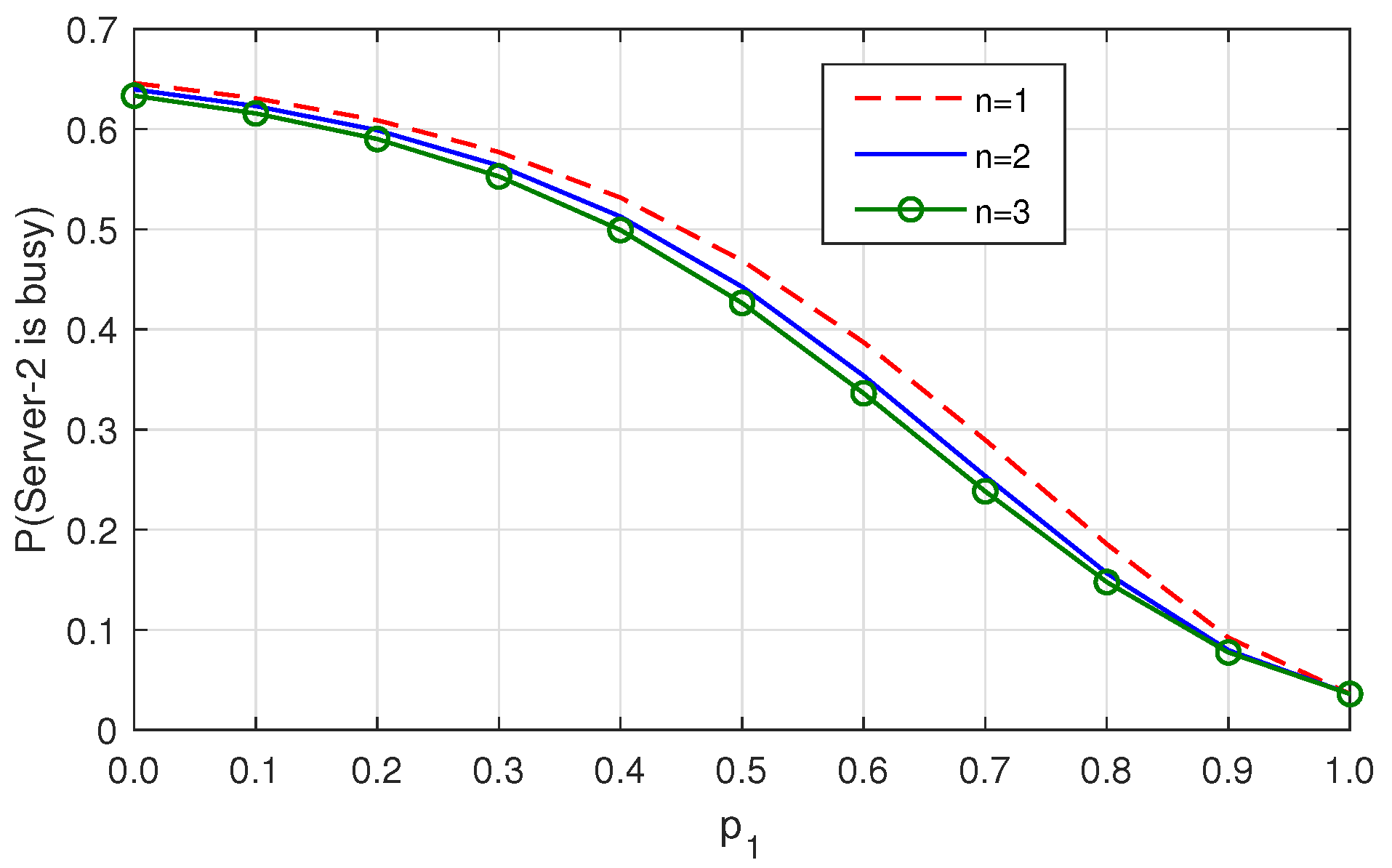
Figure 13 represents the probability of Server-2 being busy under the influence of parameters
and
. If we increase the threshold level, the probability of Server-2’s busy period will decrease. Since the probability,
reduces the number of home delivery services when it increases, Server-2’s probability of a busy period will decrease. On the other hand,
Figure 14 represents the probability of Server-2 being busy under the influence of parameters
and
. Here, we can observe that when
increases, the probability of Server-2’s busy period decreases, whereas
causes the increase in the busy period if it increases.
Figure 15 and
Figure 16 explore the probability of Server-1 and -2 being busy under the influence of parameters
and
, respectively. All the parameters involved in these figures increase both servers’ probability of the length of their busy period when they are increased.
Table 1 shows that when we increase
, the probability of Server-1 and -2 being busy increases.
Looking into the Zomato food delivery application, one can see that if the number of orders increases for a particular food, the food preparer and the delivery person are always busy until the last order is delivered. Thus, this study will be helpful for real-life businesses.
Example 3. The influence of parameters on the expected number of home delivery products:
This example explains the effect of the number of door-to-door delivery products available in the system for delivery under the parameter variation shown in
Table 2.
When we increase , the expected number of available items for door-to-door delivery increases. Every arriving customer in the system must purchase an item when they leave. Each of them has Bernoulli’s choice of a door-delivery option. So, the arrival rate influences the number of home delivery products in a direct way.
The defective rate of the product reduces the current stock level if it increases so that the sales of an inventory slow down. Following this, one may see that the expected number of home delivery products starts decreasing, as we predicted. If the replenishment happens quickly, Server-1 works continuously whenever he finds a positive queue. This means that the expected number of home delivery products will increase.
As the delivery server serves door-to-door delivery of the carried out product, the number of home delivery products in the system reduces. If we assume , then the number of home delivery products remains unchanged. On the other side, it increases the expected number of home delivery products if increases. If we increase the value of , we can observe that the number of home delivery products reduces because the number of door delivery services provided by Server-2 increases due to the self-vacation interruption. If , then Server-2 does not go for door delivery and causes an increase in the number of home delivery products in the system. It means that Server-2 will do his job upon the compulsory vacation interruption (number of home delivery products reached ).
According to the number of items available for home delivery in the system, the system manager can arrange the vehicle and delivery person for home delivery. This discussion will be helpful to such types of businesses in order to provide fast and secure service to customers. Thus, the calculation for the number of home delivery orders is used in pharmacies, online shopping, home appliance stores, and so on.
Example 4. Analysis of the number of customers present and lost in the waiting hall:
From
Table 3, the expected number of customers in the waiting hall and their loss are to be discussed with various parameters:
First, when we increase the size of the waiting hall, the expected number of customers in the system will increase. On the other hand, we see that the expected number of lost customers in the system will be reduced.
One has to implement two important strategies to reduce customer loss. One is to increase their service speed and expand the size of the waiting hall.
The arrival parameter increases the expected number of customers in the waiting hall and their loss if it increases.
If we increase , the current stock level increases. So, in the waiting room, Server-1 sells a product to a waiting customer. In such a way, the number of customers in the waiting hall is reduced. As the length of the queue decreases, the new customer will get a space in the queue. Therefore, the customer’s loss is reduced.
The parameter contributes to the customer being present in the waiting hall and losing them if it increases because if the current stock level drops, the customer will have to wait in the waiting hall until replenishment happens. So, the new incoming customer faces the no-space issue. The service rate will make a major contribution to reduce the number of customers present in the waiting hall and their loss to the system.
Table 1 shows that the number of customers in the waiting hall and the customer loss rate decrease when we increase
S.
In real life, every businessperson faces the challenge of reducing queue congestion and customer loss. These two factors will have a greater contribution to determining the company’s cost and profit. In such a way, one can apply this discussion in a mobile store, healthcare system, and so on to reduce congestion and avoid customer loss.
Example 5. An investigation on MIL, ERR and EPR: Table 4 gives the following impressions about MIL, ERR and EPR: If increases, then the mean inventory level is reduced. This is because every arriving customer buys one product from the system. This implies that the current stock will be reduced. Similarly, the expansion of the waiting hall’s size matters the same. When we expand the size of the waiting hall, more customers will arrive at the system. Therefore, the current stock level is reduced. It causes an inventory shortage. So, the mean reorder rate is increased. Since more customers purchase the product from the system, the available stock level is very low. Thus, the expected perishable rate is reduced.
Generally, increases the stock level, reduces the reorder level, and increases the mean perishable rate if it increases. Since the replenishment always produces Q items at a time in the system, the necessity of reordering is not required. Due to the present stock level, the mean perishable rate will increase.
The parameters
and
are inversely proportional to each other, and the same thing is again confirmed by
Table 4.
Further, Server-1’s service completion shows that items will be depleted one at a time. For every service completion, the current stock level is continuously reduced, which implies that the mean inventory level also becomes reduced. Since the current stock level is decreased, the mean perishable rate of the available product is also decreased.
When we observe a pharmacy, some medicines will expire. However, for finding the expected stock level, replenishing the medicine, or throwing out expired medicine, this study is certainly a useful one.
Example 6. Table 5 represents self and compulsory vacation interruptions under the parameter variation. As we reduce the service time per customer, the number of home delivery products increases. According to this increment, the expected self-vacation interruption rate for Sever-2 increases.
Supposing that the average arrival rate of a customer entering the waiting hall increases, the number of purchased items also increases. It leads to an increase in the number of home delivery products.
If we increase the threshold level of the compulsory interruption, Server-2 will have a heavy workload. To reduce such a workload, he terminates the vacation period.
The customers’ decision to choose the home delivery service increases the number of home delivery products in the system. This causes an increase in the average self-vacation interruption rate.
Server-2’s decision to continue the home delivery service at the last service completion epoch will increase the average self-vacation interruption rate.
As we extend the threshold level, the expected rate of compulsory vacation interruption is reduced because it increases the vacation duration of Server-2 and so the compulsory vacation interruption is delayed.
Both the service rate and the arrival rate cause an increase in the number of compulsory vacation interruptions on Server-2 since both rates increase the number of home delivery products in the system.
At the end of service completion on Server-1, the customer choosing the home delivery service option causes an increase in the number of home delivery products in the system. So, the number of home delivery products exceeds the threshold level.
Due to the self vacation interruption of Server-2, the number of home delivery products will reach the threshold level slowly. Thus, the average compulsory vacation interruption rate is reduced.
From the observation in
Table 5, the vacation offer given by the system manager will motivate the server to work more. After one fine period, he will terminate his vacation duration voluntarily. This will help us to provide a good home delivery service in a short period of time. Furthermore, due to the fast delivery service, the customer will have a good impression of the system’s activities.
Economical Implications in Real Life
The concept of a door-to-door delivery service facility in an SQIS is a new attempt. This idea is considered based on the real-life experience that was obtained during the curfew period due to the pandemic situation (the spread of the coronavirus (see [
28])). Noticeably, people have started ordering even food items online. Online businesses have started to send orders to customers’ doors by using a delivery server. However, the concept of a door-to-door delivery facility has been around for a long time, and it is a service provided to customers by many retailers as well as manufacturers. For example, refrigerators, air conditioners, furniture, etc., require a door-to-door delivery facility. The important matter is that many companies offer their customers the opportunity to receive a door-to-door delivery service at a low cost. According to this offer, the customer chooses a company to purchase the product from. When purchasing a large product, the transportation cost is likely to be high. Many customers are not willing to pick up the purchased product by themselves. Mostly, they choose a door-to-door delivery facility because the corresponding shop will do it at a low cost. In such a way, this proposed stochastic modeling in a queuing-inventory system will be very helpful to all business personalities of a retailer shop, wholesaler shop, and manufacturer.
7. Conclusions
This paper introduced and discussed the home delivery service facility in a stochastic queuing-inventory context. According to the assumption made in the model description, the finite generator transition matrix was formed, and the unique stationary probability was computed. Using this vector, we calculated the necessary system performance measures and the expected total cost of the proposed model. The expected total cost is optimized as the function of S and s for each parameter variation of and When approaches zero, this model comes under the ordinary queuing-inventory system. If , all the customers must opt for the home delivery option. As we expected, the increased number of home delivery products increases the flow of customers into the system. Due to the increase in arrival flow, the probability of Server-1 and -2 being busy also increases. The reorder rate controls the customer’s average loss rate when it increases. Additionally, it reduces the customer’s waiting time if it increases. If we control the perishable rate of an item, the customer’s loss rate and waiting time can be reduced. Self vacation interruption helps the server reduce the workload in the home delivery service process. One can observe that the compulsory interruption of the delivery server’s vacation period can be reduced if we increase the threshold level. All business tycoons will gain insight from an analysis of the likelihood that Server-2 is on vacation or busy fulfilling the door-to-door delivery service. The effect of P(Server-2 is busy) when the parameters are varied together is graphically illustrated. Due to this effect, one may plan a new strategy for improving the door-to-door delivery facility. In the future, we can extend this door-to-door service facility with multiple delivery servers. Additionally, we can assume a phase-type distributed service for home delivery. Further, this work can also be extended to online shopping contexts.


 ,
, 


