The comparison of the models included two stages: the first stage consisted of the step size experiment, for which the purpose was to elect the appropriate step size value according to the experimental results; the second stage consisted of testing the predictive power of the model using additional test data after the step size was fixed. Comparative experiments were conducted on the Bi-LSTM, EMD-LSTM, STL-LSTM, and JUST-STL-Bi-LSTM models. JSBL represents the JUST-STL-Bi-LSTM model proposed in this paper. The step size experiment included a dataset of the daily mean temperature levels of 34 provincial capital cities in China.
3.3.1. Step Size Experiment
When the step size values were set to 20, 30, and 40, the RMSE values of the four models with different step sizes were obtained, as shown in
Table 1. The RMSE value of the JSBL model was 0.2187 when the step size was 40. The values obtained for the other models were 4.3997, 2.5343, and 0.9336. We can observe that the RMSE result for the JSBL model is minimal.
As can be observed in
Table 1, the prediction accuracy of the model combined with the decomposition algorithm is significantly higher than that of the model lacking a decomposition algorithm, indicating that the combination of an appropriate decomposition algorithm can effectively improve the prediction accuracy of the algorithm. It can also be observed in
Table 1 that the prediction accuracy of the Bi-LSTM model changes a little when the step size is different. The accuracy of the STL-LSTM model and the model presented in this paper produced the best results when the step size was 40.
The MAEs of the four models with different step sizes are presented in
Table 2. According to
Table 2, the MAE of each model changes little when the step sizes are 20 and 30, and the JSBL model presents the best MAE when the step size is 40. R
2 is presented in
Table 3. For a smaller step size, JSBL combined the JUST and STL algorithms, which needed to learn more features, the model training process was slower, and some features had not been learned at the end of the cycle. Therefore, the prediction accuracy of the JSBL model may be reduced when incorporating smaller step sizes. In contrast, the STL-LSTM model needs to learn fewer features, and a smaller step size can satisfy the training demand; a continuous increase in the step size instead leads to the occurrence of scattering or oscillation in the model’s training process.
From the observation of
Table 1,
Table 2 and
Table 3, it can be determined that when the step size is 40, the performance of the algorithm proposed in this paper is successfully reflected, and other models also perform well when incorporating this step size. Therefore, the step size of 40 was selected to conduct subsequent model evaluation experiments.
3.3.2. Model Evaluation
In the model evaluation experiment, the daily mean temperature dataset of 60 random cities located in China was used. The model evaluation experiment consisted of four stages. Firstly, each model was evaluated using the evaluation metrics for the dataset. Secondly, in order to test the sensitivity of the model to the data, the evaluation indexes of each model were tested using the cumulative distribution function. Thirdly, in order to display the intuitive prediction effect of the model, a longer length of data was randomly selected to display the prediction effect of the model. Finally, in order to successfully present the differences in the prediction’s details, the data with lengths of 60 were selected to compare the prediction effects of each model.
Several models were evaluated using additional daily mean temperature datasets to test the predictive power of the models. For our convenience, numbers 1–60 were used in this study to indicate the corresponding site of each city. For the changes in the R
2 values in the additional test dataset, only the changes in 10 random sites were presented in this study, as shown in
Table 4. It can be observed in
Table 4 that the R
2 values for all models were higher than 0.9, which indicates that all the models had a certain ability to perform predictions. Secondly, the JUST-STL-Bi-LSTM (JSBL) model presented the highest fitting coefficient, indicating that it attained the best fitting degree.
The RMSE and MAE values of the four models on the additional test datasets are presented in
Figure 7 and
Figure 8, respectively.
The following information can be observed in
Figure 7 and
Figure 8. Firstly, the RMSE and MAE values of the model presented in this paper are both the lowest. Secondly, the RMSE and MAE values of the JUST-STL-Bi-LSTM and STL-LSTM models fluctuate, almost in the shape of a horizontal line, and present strong resistance to sensitive data. However, the Bi-LSTM and EMD-LSTM models presented a wide fluctuation range and high sensitivity to the data. Therefore, the model proposed in this paper was superior to the other models in its ability to perform predictions.
The average performance indexes of several models on additional test datasets were calculated during the experiment, including the RMSE, R
2, and MAE. The JSBL model performed the best on the additional 60-site test datasets, followed by the STL-LSTM, EMD-LSTM, and Bi-LSTM models. The average RMSE, MAE, and R
2 values of each model are presented in
Table 5.
The average RMSE and MAE values only reflected the comprehensive performance of the model; however, they could not present the sensitivity of the model to the data. In order to present the sensitivity of several models to the data, the cumulative distribution function (CDF) was used to calculate the distributions of the RMSE and MAE values. The cumulative distribution function is defined as Formula (12), where
represents the real variables,
is the probability distribution of all
values, and
represents the probability. The cumulative distribution function is defined as the sum of the probabilities of all variables less than or equal to
.
This study conducted a CDF analysis on both RMSE and MAE.
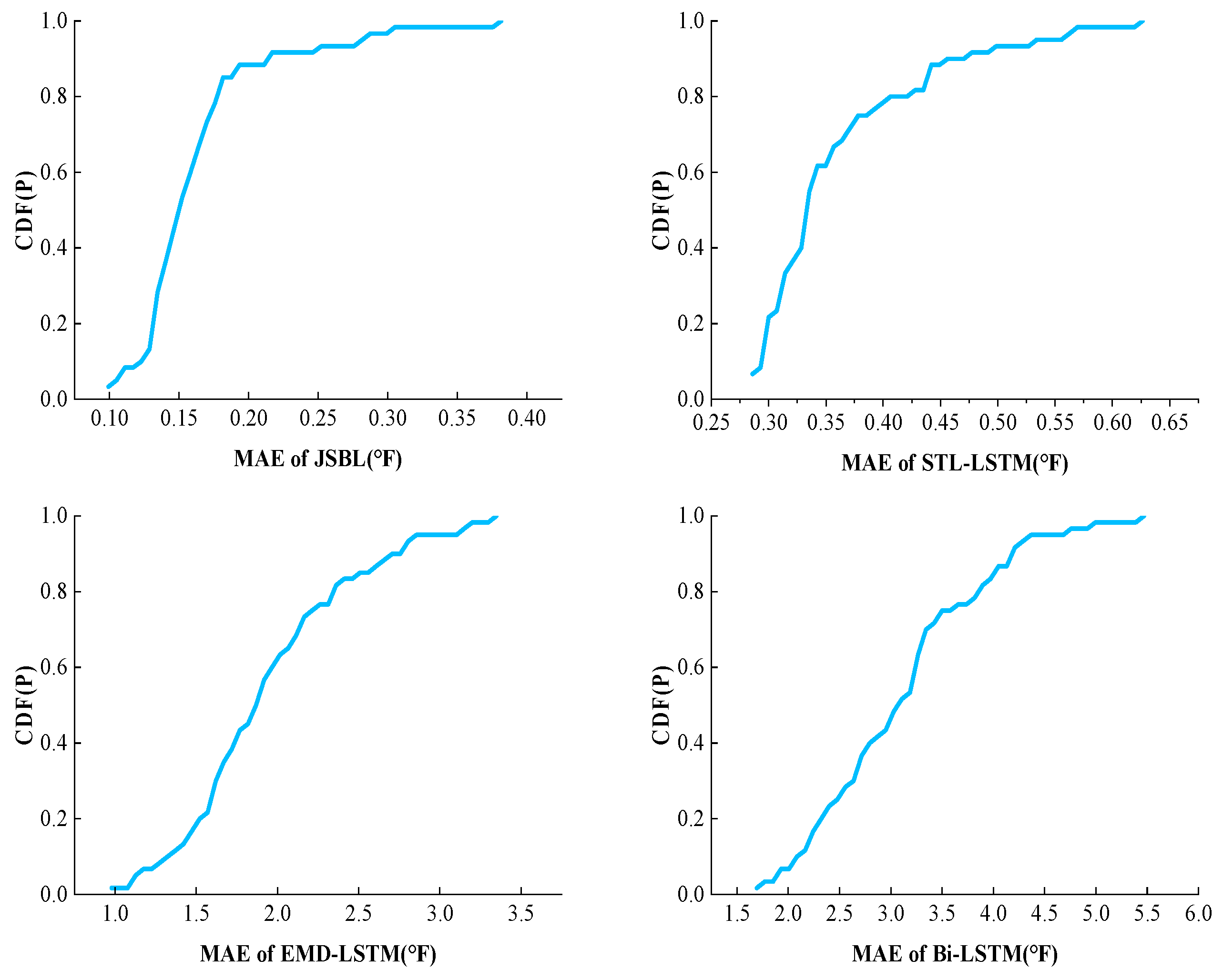
Figure 9 presents the CDF changes presented the RMSEs of the four models. By observing
Figure 9, it can be determined that most of the errors produced by the JSBL model are concentrated less than a value of 0.4, where the probability is very close to 100%, indicating that most of the errors exhibited are less than 0.4. This result indicates that, for most of the data obtained, the prediction errors produced by the model are close, the sensitivity to the data is not high, and the adaptability is good. For the STL-LSTM model, concerning all the error data, the majority of the errors were less than a value of 0.75. For the remaining two models, the CDF curve changed more uniformly, indicating that the error distribution in the error dataset was more evenly distributed. The proportion of smaller and greater errors was close, indicating that the model was highly sensitive to the input data.
Figure 10 presents the CDF changes observed for the MAEs of the four models.
The Kolmogorov–Smirnov predictive accuracy (KSPA) method can accurately test whether a statistically significant difference between the prediction errors of the two models is present [
33,
34]. We used KSPA to test whether the prediction errors produced by the JSBL model were statistically significantly different from those produced by the other models. We attained statistics for the RMSE values only. The
-value of the two-sided KSPA test was less than 0.05, indicating that there was a statistically significant difference evident between the prediction errors produced by the two models. The
-value of the one-sided KSPA test was less than 0.05, indicating that the JSBL model produced a lower random error value than the other models. The test results are presented in
Table 6.
-values less than 0.05 refer to the 95% confidence level. As can be observed in
Table 6, all the
-values are within the 95% confidence level range, indicating that our model produced a lower random error than the other models.
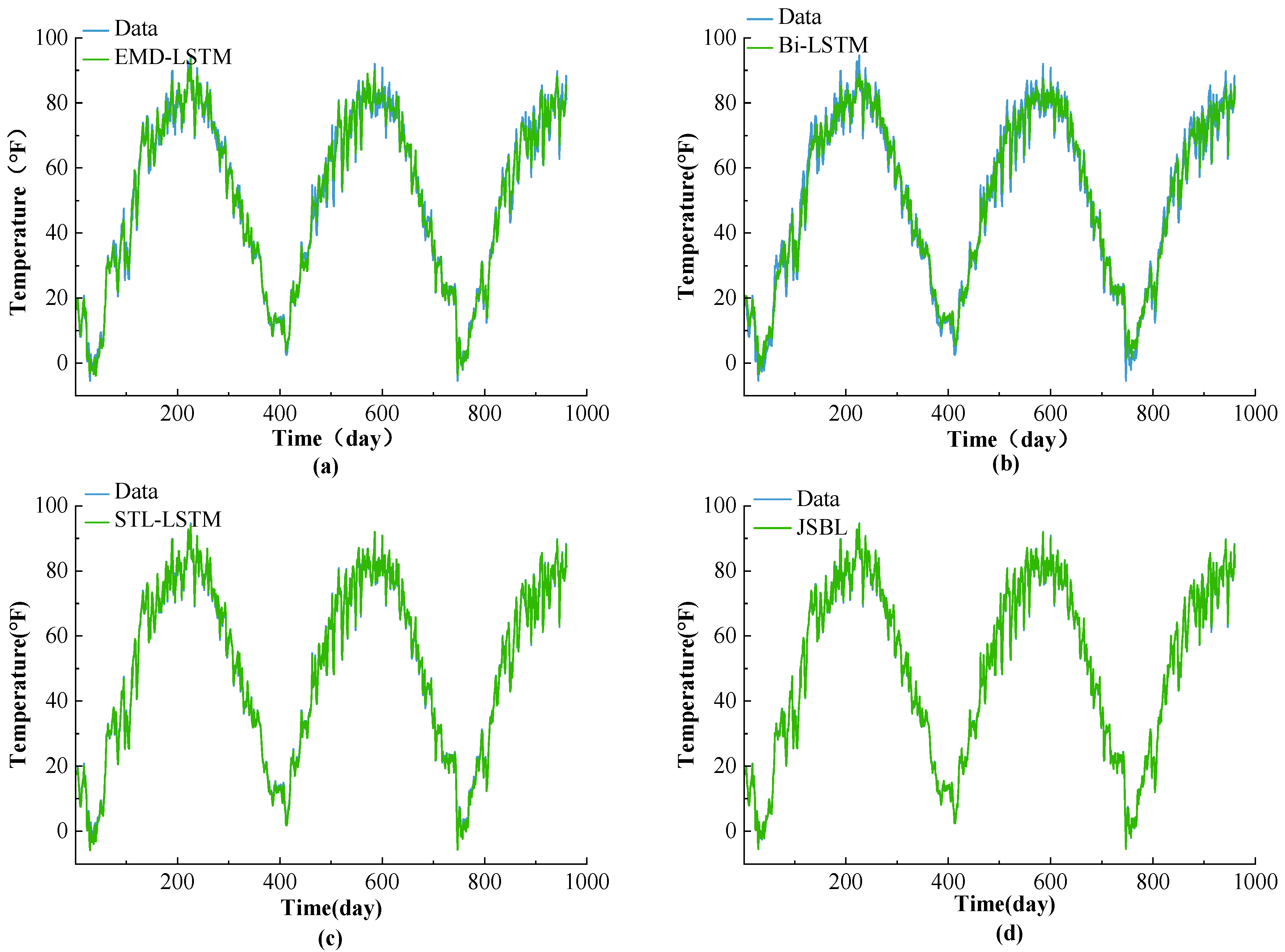
To accurately display the prediction effect of each model, the test data with a sequence length of 960 days were randomly selected to perform a comparison, as shown in
Figure 11. In
Figure 11, it can be observed that the Bi-LSTM and EMD-LSTM models produce poor prediction effects. A considerable error between the real and predicted values for this model is evident. The JSBL and STL-LSTM models presented prediction effects. The error evident between the predicted and true values is small. At the same time, it can be observed that the JSBL model forecasted the relevant details more appropriately than the STL-LSTM model. The results show that the JSBL model has better practicability and effectiveness characteristics.
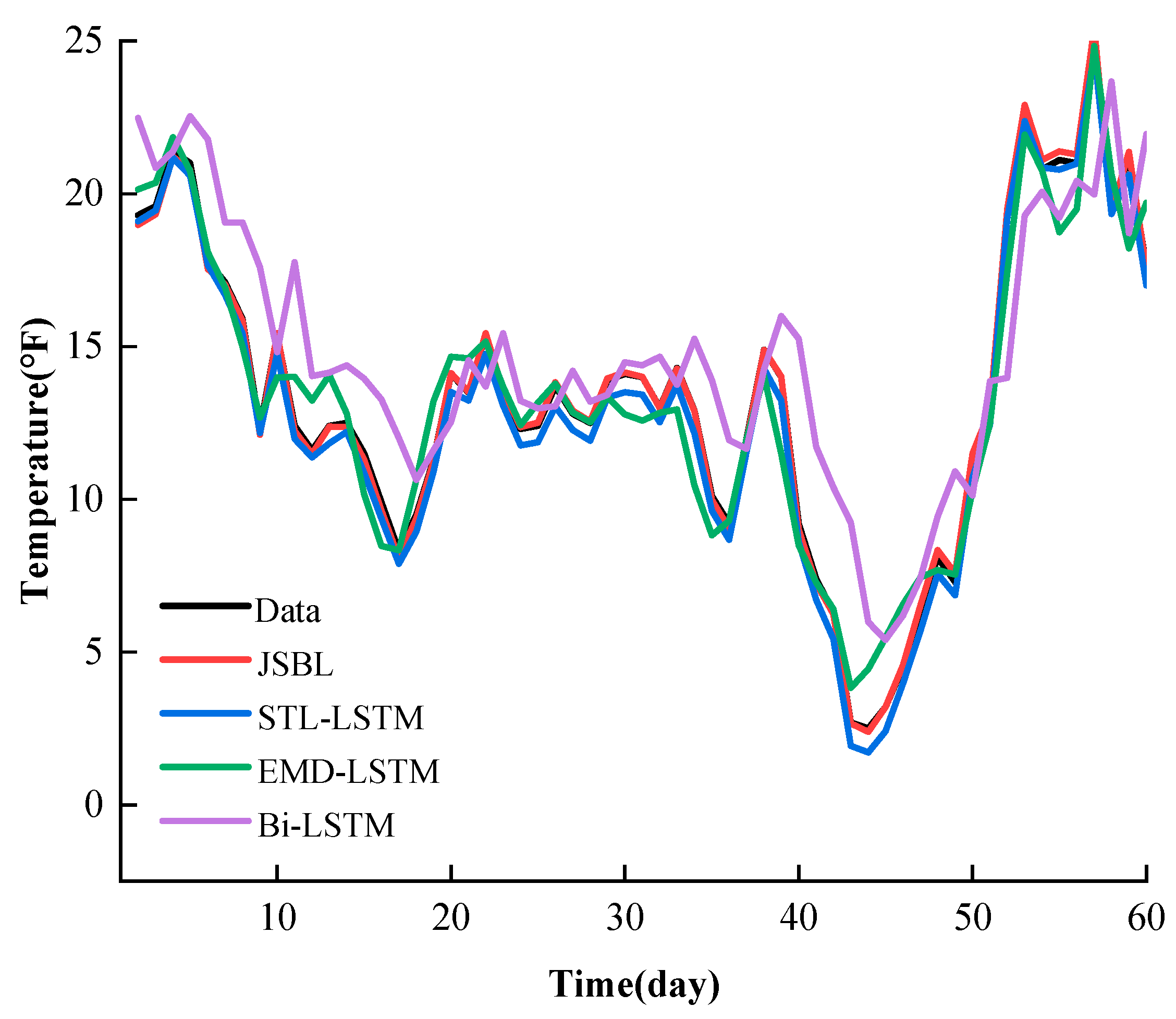
In order to present the prediction results for each model, the data with a time length of 60 days were randomly selected for a post-prediction comparison. As shown in
Figure 12, we can observe that the JSBL model is much better at predicting the relevant details. The predicted value is much closer to the true value. The JSBL, STL-LSTM, and EMD-LSTM models present light hysteresis, while the Bi-LSTM model presents strong hysteresis. Then, the predictions of the STL-LSTM, EMD-LSTM, and Bi-LSTM models successively declined in their accuracy.


