Research on Distribution Optimization of Emergency Perishable Materials Considering Periodic Changes in Freshness

Abstract

The distribution of emergency perishable materials is crucial for rescue operations in disaster-stricken areas. However, the freshness of these materials changes over time, affecting the quantity of materials that can be distributed to demand points at different stages. To address this issue, this paper proposes a novel approach. Firstly, a piecewise function is constructed to describe the impact of freshness on the quality and quantity of emergency perishable materials at different time stages. Secondly, the paper establishes a vehicle distribution optimization model with the goal of maximizing the sum of the freshness of all emergency perishable materials delivered to different disaster-affected locations, taking into account the different minimum freshness constraints for the same kind of materials in different locations. Thirdly, an approximate algorithm is designed to solve the model, with the time complexity and the upper and lower bounds of the approximate ratio analyzed. Finally, an example analysis is conducted to demonstrate the validity of the proposed model and algorithm.

1. Introduction

In the aftermath of a sudden disaster, the disaster site requires a significant amount of emergency rescue materials, including perishable items such as blood, vegetables, milk powder, meat, and more. These emergency perishable materials are highly time-sensitive and require prompt delivery [1]. As a result, delivering high-quality and fast emergency perishable materials to disaster-stricken areas has become a crucial issue for scholars and business experts to address.

At present, the research on the vehicle routing problem of perishable materials mainly focuses on two aspects. One is the research that considers that the quantity of perishable materials will change with time during the distribution process. Generally, the corruption rate is used to measure the loss of quantity of perishable materials in a unit time, and there are only two states of corruption and non-corruption when the materials are delivered to the demand point, regardless of the degree of corruption of each emergency perishable material. With the goal of minimizing the cost of corruption, an optimization model for the distribution of perishable materials is established. The other is the research that considers the quality of perishable materials that will change over time during the distribution process. Generally, the freshness is used to measure the change of the quality of perishable materials over time; the change of the quantity of emergency perishable materials is not considered, and the discrete function is used—a linear or nonlinear continuous function that measures changes in freshness. Aiming at the minimum distribution cost or the minimum loss of freshness, an optimization model for the vehicle distribution of perishable materials is established.

In practical scenarios, the minimum freshness constraints for the same kind of emergency perishable materials at a demand point can vary based on the degree of damage and the distance between the demand point and the rescue center. Furthermore, the change characteristics of freshness for emergency perishable materials differ across different time stages, and the fitting functions for these changes also vary. As the freshness of emergency perishable materials decreases, there comes a point where the physical and chemical freshness indicators of the materials continue to decline, rendering them inedible and useless. As a result, changes in freshness can significantly impact the quantity of materials that can be distributed.

This study addresses the limitations of previous research by constructing a piecewise function that describes the changes in the quality and quantity of emergency perishable materials across different time periods. Additionally, to account for the varying minimum freshness constraints of the same kind of materials at different disaster-stricken points, we propose a vehicle distribution optimization model. The objective of this model is to maximize the freshness of all emergency perishable materials delivered to the disaster-stricken points.

The vehicle distribution optimization problem is known to be a challenging NP-hard problem [2], as an exact algorithm cannot solve it, and finding the optimal solution is not possible. Therefore, only a sub-optimal solution can be obtained. In contrast to heuristic algorithms, approximate algorithms [3,4] can quickly find reasonable solutions and only need to prove the quality and running time bounds of the solution. Thus, using an approximate algorithm can guarantee the quality of the solution. In this article, we propose an approximation algorithm to solve the constructed model, calculate the time complexity of the algorithm, and analyze its approximation ratio.

The paper is organized as follows. The second section presents the related work. The third section presents the methodology, including the problem formulation, the model design, and the solution. The following section presents a case analysis. The last section presents the conclusion and future directions.

2. Related Work

Vehicle Routing Problem: The Vehicle Routing Problem (VRP) was first proposed by Dantzig et al. in 1959 and aims to seek the best vehicle path for a series of given loading points and unloading points [5]. Common constraints include demand for goods, vehicle capacity, and time window limitations. The objective function of VRP is artificially set, such as the shortest distance, the least cost, the last time, and the least number of vehicles used. In the ensuing decades, extensive work was conducted on VRP. These previous studies investigated VRP with perishable materials considering the actual demand.

The relevant literature on this topic can be broadly categorized into three aspects: firstly, research on distribution optimization for perishable materials that may deteriorate over time during the distribution process; secondly, studies on distribution optimization that take into account the changing quality of perishable materials during the distribution process; and finally, research focused on the development of freshness functions for perishable materials.

In research on the distribution optimization of perishable materials considering freshness, the corruption rate is a measure of the loss of perishable materials over time, with only two states of corruption and non-corruption upon delivery to the demand point.

Shiva Zandkarimkhani [6] developed a dual-objective mixed integer linear programming model for the supply chain network of perishable materials under demand uncertainty, with the aim of minimizing the total cost and demand loss. A new hybrid approach was designed to solve the proposed model, and its effectiveness was evaluated using data from Avonex. Zheng Liu et al. [7] constructed an integer programming model to minimize the sum of inventory cost, penalty cost, perishable material damage cost, and refrigeration cost and conducted an example analysis. The simulation results of the genetic algorithm and the hybrid algorithm were compared, and the hybrid algorithm was found to be more effective. Yuqiang Feng et al. [8] studied the location allocation of perishable material distribution centers, with the goal of minimizing the total cost, including rental costs, transportation costs, and fuzzy expected penalty costs resulting from shortages caused by the corruption of perishable materials. They also determined the quantity and location and designed a distribution plan for perishable materials. Xiao Liu et al. [9] aimed to minimize the total response time and total operating cost of perishable materials, considering the corruption rate of emergency perishable materials and the emergency supply constraints. They established a discrete-time mixed integer linear programming (MILP) model and solved it.

In research on the distribution optimization of perishable materials considering freshness, the freshness function is commonly used to describe changes in the quality of perishable materials over time. Jing Chen [10] proposed a freshness-based strategy and a quantity-based strategy to find the optimal preset scheduling quality level, optimal input preservation effort, and optimal scheduling quantity. These strategies integrate freshness-keeping work decisions to construct a corresponding integrated stochastic model for perishable product transportation.

Yufeng Zhou [11] aimed to minimize the transshipment time of perishable materials and maximize freshness. Based on recursive equations, they provided the status of demand for two types of perishable materials under two inventory distribution strategies (FIFO and LIFO) with a transfer equation. They established an optimal model for the perishable material transfer problem and designed a discrete event system simulation (DESS) framework. The effectiveness of the decision-making method and the EWA inventory strategy was verified by numerical simulation. B. Zahiri [12] established a mathematical model for designing the perishable material supply chain network considering the freshness, substitutability, and quantity discount of perishable materials. A new robust likelihood optimization method was introduced, and the proposed optimized network was discussed to minimize the total cost of the supply chain network and maximize the minimization of demand. Ali Rahbari [13] proposed two robust models to solve the vehicle routing and scheduling problem of cross-docking perishable products when the travel time of outbound vehicles and the freshness of products are uncertain. They proved that considering only one goal will sacrifice the other, and the L1 metric makes appropriate tradeoffs. Hao Zhang [14] proposed an improved genetic algorithm that considers the nature of fresh products and the characteristics of urban logistics systems. The algorithm aims to maximize the freshness of perishable materials while minimizing the total cost of distribution. An iterative optimization procedure is used to determine the optimal route, reducing the computational complexity in searching for an optimal solution. Yan Li [15] constructed a green vehicle routing optimization model for cold chain logistics to minimize the freshness loss of perishable materials. They used intelligent optimization algorithms to solve routing problems in actual cases. Related work in this direction is summarized in Table 1.

Table 1. Summary of previous work. Yes indicates that the method is used.

Refs.	Only Quality Loss	Only Quantity Loss	Both Quality and Quantity Are Lost
Shiva Zandkarimkhani [6]		Yes
Xiao Liu [7]		Yes
Zheng Liu [9]		Yes
Jing Chen [10]	Yes
Yufeng Zhou [11]	Yes
B. Zahiri [12]	Yes
Ali Rahbari [13]	Yes
Hao Zhang [14]	Yes
Yan Li [15]	Yes

Freshness function: The freshness function of perishable materials refers to the direct effect of time on the physical and chemical properties of these materials, resulting in the attenuation of material quality, decay, and eventual waste. Rong et al. [16] proposed a linear function of time to describe the freshness of perishable materials at a specific temperature. Jedermann et al. [17] used an exponential decay function to describe the decay of perishable materials over time at a certain temperature. Amorim et al. [18] used the ratio of the difference between the shelf life of perishable materials and the time of delivery to the demand point to the shelf life of perishable materials to describe the relationship between the freshness of perishable materials over time. Rabbani et al. [19] considered the initial shelf life to be constant at 100% and used the ratio of the difference between the shelf life and the delivery time of perishable materials to the shelf life to determine the freshness of perishable materials. Mejjaouli and Babiceanu [20] classified products as good or spoiled based on specific probabilities for each shipping scenario. Hsiao [21] constructed a linear freshness function of perishable materials at a specific temperature based on Rong’s research and used the reciprocal of the shelf life of perishable materials to deduce the degree of decline in the quality of perishable materials per unit time. Stellingwerf et al. [22] used the Arrhenius equation to describe the decay of perishable material freshness over time at a certain temperature.

When studying vehicle route distribution optimization in the context of perishable materials, there is no standardized method for describing quality change over time. Discrete freshness functions, as well as linear or nonlinear continuous freshness functions, have been used to describe the law of perishable material quality change over time. However, in practice, the freshness of emergency perishable materials may change in stages, which can affect the quantity of materials. In the first stage, the freshness decreases slowly while the quality of the materials remains stable and the quantity remains unchanged. In the second stage, the freshness decreases rapidly, and while the material quality is lost, it can still be accepted by the demand point, leaving the quantity unchanged. In the third stage, the freshness decreases at an accelerated rate but does not drop to zero, resulting in a total loss of supplies. Related work in this direction is summarized in Table 2.

Table 2. Summary of previous work. Yes indicates that the method is used.

Refs.	Discrete Function	Linear Function	Arrhenius	Exponential Function
Rong et al. [16]		Yes
Jedermann et al. [17]				Yes
Amorim [18]	Yes
Rabbani et al. [19]	Yes
Mejjaouli and Babiceanu [20]	Yes
Hsiao [21]	Yes
Stellingwerf et al. [22]			Yes

Our insight: This study aims to address not only the changes in quality but also the changes in quantity of emergency perishable materials during distribution. To achieve this, a segmented freshness function is constructed to describe the impact of materials on both quality and quantity at different time stages. Additionally, the model takes into account the minimum freshness requirements of the same emergency perishable materials at the disaster-stricken point. An optimization model is established to distribute emergency perishable materials while maximizing the sum of point freshness. An approximate algorithm is designed to solve the model, and the effectiveness of both the model and algorithm is verified through examples.

3. Methodology

This section first presents the problem definition. Second, this section presents the designed mathematical model for the problem. Finally, this section presents the designed solution for this mathematical model. The key notations used in this paper are listed in Table 3.

Table 3. Summary of key notations.

Notation	Description
$v_0$	Distribution center for emergency perishable materials
$v_i$	Demand points for emergency perishable materials
$\vartheta$	The average speed of delivery vehicles
$d_{ij}$	The shortest path distance from $v_i$ to $v_j$
$q_i$	The demand quantity of demand point $v_i$
$Q^{*}$	The maximum loading capacity of the delivery vehicle
$t_{ij}$	The delivery time of the vehicle from $v_i$ to $v_j$ along the shortest route
$t_{0i}$	The delivery time of the vehicle from $v_0$ to $v_i$ along the shortest route
$F\left(t_{0i}\right)$	Measuring function of the freshness of emergency perishable materials
$f_i$	The minimum requirements for the freshness of materials at $v_i$
$t_1$	The fresh period of emergency perishable materials
$t_2$	The second fresh period of emergency perishable materials
T	The duration of the freshness of materials drops to zero
$F_i$	The freshness of emergency perishable materials at $v_i$
$x_{ij}$	The decision variable

3.1. Problem Formulation

Let $G=(V,E)$ be an undirected network. Let $V=\left\{v_0,v_1,v_2,\dots ,v_n\right\}$ be the set of points in $G=(V,E)$. Let $v_0$ be the distribution center for emergency perishable materials. Let $v_1,v_2,\dots ,v_n$ be demand points. Let $E\left\{e\left(v_i,v_i\right)\mid v_i,v_i\in V\right\}$ be the set of edges in $G=(V,E)$. Emergency rescue center $v_0$ has an emergency perishable material that must be distributed to each demand point $v_i$. Let $q_i$ be the demand for the emergency perishable materials from the demand point $v_i$. Let $d_{ij}$ be the shortest distance from demand point $v_i$ to $v_j$. Let $t_{ij}$ be the delivery time of the vehicle from demand point $v_i$ to $v_j$ along the shortest path. Let $F\left(t_{0i}\right)$ be a measure function of the freshness of emergency perishable materials. Let $t_{0i}$ be the delivery time of the vehicle from $v_0$ to demand point $v_i$ along the shortest path. Let $f_i$ be the demand point $v_i$’s minimum freshness requirements for emergency perishable materials. Let $F_i$ be the freshness of emergency perishable materials at demand point $v_i$. The distribution center currently has a vehicle with a maximum load of $Q^{*}$ and $Q^{*}\ge {\sum }^n{q}_i$. The problem to be solved is described as follows. We schedule vehicles to travel at average speed $\vartheta$ from distribution center $v_0$. Vehicles deliver materials to various demand points. We expect to compute the delivery route of the vehicle to maximize the sum of the freshness of all demand points.

3.2. Mathematical Model

The measure function for the freshness: The freshness of emergency perishable materials is a comprehensive expression of their quality characteristics, which are determined by their physical and chemical freshness indicators.

Perishable materials have varying freshness measurement functions in practice. Two types of freshness functions are commonly used, namely the segmented freshness measurement function and continuous freshness measurement function. The continuous freshness function assumes that the freshness of perishable materials decays continuously over time. The forms of the continuous freshness function typically include linear, exponential, and polynomial freshness functions.

Emergency perishable materials undergo two stages of freshness decay. During the first stage, which is due to short delivery times, the freshness decay rate is relatively slow and the material quality remains stable. This stage can be approximated as a constant decay rate, with a linear relationship between freshness and time. In the second stage, as time increases, the material quality deteriorates gradually. The deteriorated part affects the remaining material, accelerating its decay. The freshness attenuation rate in this stage increases continuously and can be approximated by a quadratic function describing the relationship between freshness and time. The resulting freshness measurement function is shown in Figure 1. The measure function of freshness is given by

$$F^{\prime }\left(t_{0i}\right)=\left\{\begin{array}{c}1-\beta t_{0i}, 0\le t_{0i}\le t_1\hfill \\ 1-\frac{t_{0i}^2}{T^2}, t_1\le t_{0i}\le T\hfill \end{array}\right.$$

(1)

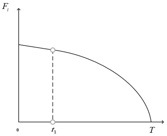
Figure 1. The measure function of the freshness of emergency perishable materials.

In actual distribution, the emergency perishable materials deteriorated severely before their freshness dropped to zero. At this time, the material loses its reason for distribution. Thus, we improve the above freshness measure function.

We divide the change of freshness into three stages. The first stage is the freshness period ($0\sim t_1$), as shown in Figure 2. At this time, the emergency perishable materials are in the freshness period and the freshness decreases slowly, which can be regarded as a constant decay rate. We use a linear function to measure the change of freshness, and this stage is the best period for material distribution.

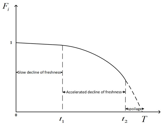
Figure 2. The improved measure function for freshness.

The second stage is the secondary freshness period ($t_1\sim t_2$). At this time, the emergency perishable materials are in the sub-fresh period, and the decay rate of freshness in this stage is gradually increasing. Thus, we use a quadratic function that opens downward to describe the decay rate. Although this stage is not the best period for material distribution and the loss of freshness is large, the material still has value.

The third stage is the metamorphic period ($t_2\sim T$). At this time, the emergency perishable materials are in the deterioration period. Although the freshness of emergency perishable materials is still declining at an accelerated rate and has not dropped to zero, emergency perishable materials have deteriorated severely and are useless at this stage.

When the material delivery time satisfies $t_{0i}\ge t_2$, all the materials are damaged. At this point, the vehicle will stop delivering emergency perishables. The improved freshness measure function of emergency perishable materials is given by

$$F\left(t_{0i}\right)=\left\{\begin{array}{c}1-\beta t_{0i}, 0\le t_{0i}\le t_1\hfill \\ 1-\frac{t_{0i}^2}{T^2}, t_1\le t_{0i}<t_2\hfill \end{array}\right.$$

(2)

where $\beta$ is the decay rate of freshness during the freshness period, $0<\beta \le 2t/T^2$, and $t_{0i}\in \left[0,t_2\right)$. $t_1$ is the freshness period of emergency perishable materials. $t_2$ is the second freshness period of emergency perishable materials. T is the time when the freshness of emergency perishable materials drops to zero. $t_1,t_2,T$ are constants. $t_{0i}$ is the delivery time of the vehicle from $v_0$ to $v_i$. The improved freshness measure function is shown in Figure 2.

The mathematical model: We begin by making the following six assumptions. First, the demand quantity at the demand point is known. Second, the distribution center has complete temperature-controlled refrigeration facilities, ensuring that emergency perishable materials are 100% fresh upon arrival and have not deteriorated in freshness. Third, emergency perishable materials are transported in ordinary vehicles at room temperature, with no changes to the environment during transportation. Any changes in freshness are solely due to time. Fourth, we do not consider the loading and unloading time of materials at the demand point. Fifth, $t_1,t_2,T$ are all constants. Sixth, the total amount of materials in the emergency rescue center is sufficient.

Moreover, we define the decision variable $x_{ij}$ as follows:

$$x_{ij}=\left\{\begin{array}{c}1,\mathrm{Vehicle}\mathrm{moves}\mathrm{from}{v}_i\mathrm{to}{v}_j\mathrm{along}{\mathrm{e}}_{ij}\hfill \\ 0,\mathrm{Otherwise}\hfill \end{array}\right.$$

(3)

Based on the above assumptions, we formulate the mathematical model associated with the decision variable $x_{ij}$.

The objective function is as follows.

$$Z=max\sum _{i=1}^n{F}_i\ast q_i$$

(4)

The constraints are as follows.

$$t_{ij}=\frac{d_{ij}{x}_{ij}}{\vartheta }$$

(5)

$$\sum _{i=1}^n{q}_i\le Q^{*}$$

(6)

$$\sum _{i=1}^n{x}_{ij}\le 1(j=1,2,3,\dots ,m)$$

(7)

$$x_{ij}=\{0,1\}(j=1,2,3,\dots ,m)$$

(8)

$$0\le F_i\le 1(i=1,2,3,\dots ,n)$$

(9)

$$0\le f_i<1(i=1,2,3,\dots ,n)$$

(10)

$$0<t_1<t_2$$

(11)

$$t_1<t_2<T$$

(12)

$$0\le t_{0i}<t_2(i=1,2,3,\dots ,n)$$

(13)

$$\sum _{i=1}^n\sum _{j=1}^n{x}_{ij}\le \left|S\right|-1,2\le \left|S\right|\le n-2$$

(14)

A description of each formula is shown in Table 4.

Table 4. Summary for formulas.

Formula Number	Description
Equation (2)	Freshness function of emergency perishable materials
Equation (4)	Maximize the freshness of all demand points
Equation (5)	Compute the transit time of vehicles along the shortest path
Equation (6)	Constraints on vehicle loading
Equation (7)	Each demand point can only be served once
Equation (8)	Constraint on the values of decision variables
Equation (9)	Constraint on the freshness
Equation (10)	Constraint on the minimum required freshness
Equations (11)–(13)	Constraint on time
Equations (13) and (14)	Avoid sub-loops

3.3. Solution

In this section, we first review the proposed solution and then analyze the time complexity and approximate ratio of the proposed solution.

3.3.1. Overview for Solution

The vehicle cannot reach some demand points within $t_2$ if it travels along the shortest path since some demand points are far away from the distribution center. Thus, we first preprocess the model to remove redundant constraints in the model. We check the transit time $t_{0i}$ of the shortest path from $v_0$ to $v_i$, and if $t_{0i}$ is greater than the transit time of the shortest path from $v_0$ to $v_i$, we remove the constraint corresponding to $v_i$. Meanwhile, $q_i=0$.

Firstly, we apply the Dijkstra algorithm to compute the shortest path from emergency rescue center $v_0$ to each demand point $v_i$. Let $P\left(v_0,v_i\right)$ be the shortest path from $v_0$ to $v_i$. Then, we compute the travel time $t_{0i}$ along the shortest path from the emergency rescue center to each demand point. Next, we compute the material freshness $F\left(t_{0i}\right)$ of each demand point, according to the freshness measurement function $F_i$ of emergency perishable materials. Then, we compare the material freshness $F_i$ of each demand point with the minimum freshness requirement $f_i$ of the demand point. If the demand point $F_i<f_i$, we delete the constraint corresponding to the demand point and make the demand $q_i=0$. If $F_i\ge f_i$, we compute the product of the freshness $F_i$ of each demand point and the demand $q_i$ of each demand point. Finally, we sort the values of $F_i\ast q_i$ and select the largest demand point of $F_i\ast q_i$ as the first demand point to be delivered by vehicles.

Secondly, we mark the first delivered demand point as the new starting point of the vehicle and use the Dijkstra algorithm to compute the shortest path from the new starting point of the vehicle to the remaining demand points. We compute the travel time along the shortest path from the new starting point to the remaining demand points and then compute the freshness of the materials at the remaining demand points. Similarly, we compare the material freshness of each demand point with the minimum freshness requirement of the demand point. If $F_i\ge f_i$, we delete the demand point. Conversely, we compute the product of the freshness $F_i$ of each demand point and the demand $q_i$ of each demand point. Next, we sort the values of $F_i\ast q_i$, and select the largest demand point of $F_i\ast q_i$ as the second demand point to be delivered by vehicles. Meanwhile, we compare ${\sum }^n{t}_{*}^{\alpha }$ and $t_2$. If ${\sum }^n{t}_{*}^{\alpha }\ge t_2$, the vehicle stops delivering. If ${\sum }^n{t}_{*}^{\alpha }<t_2$, we continue to deliver to other demand points according to the above rules. When ${\sum }^n{t}_{*}^{\alpha }\ge t_2$ or all demand points are serviced, the vehicle stops delivering. Finally, we output $x_{ij}$ and the freshness $F_i\ast q_i$ of the delivered demand points and output the sum of the freshness of all demand points ${\sum }^n{F}_i\ast q_i$. The detailed procedure for the designed solution is as follows.

Step 1. Create a set of demand points as $V_N^{\alpha }=\left\{v_1^{\alpha },v_2^{\alpha },\dots ,v_n^{\alpha }\right\}$.

Step 2. Let $v_0$ be the starting point and $\alpha =1$.

Step 3. Apply the Dijkstra algorithm to compute the shortest path $\left\{P\left(v_0,v_i^1\right)\right\}$ from the starting point to each demand point $v_i^1(i=1,2,\dots ,n)$. Record all the edges $\left\{e_P\left(v_0,v_i^1\right)\right\}$ on each shortest path, and the distance $d\left(v_0,v_i^1\right)$ from the starting point to each demand point $v_i^1$.

Step 4. Compute the travel time $t_i^1$ along the shortest path from the starting point to each demand point according to $t_{ij}=\frac{d_{ij}{x}_{ij}}{\vartheta }$.

Step 5. Compute the material freshness $F_i^1$ of each demand point according to the freshness measure function $F\left(t_{0i}\right)$ of emergency perishable materials.

Step 6. Compare $F_i^1$ and $f_i^1$ of each demand point. If the demand point satisfies $F_i^1<f_i$, we remove the demand point from set $V^N$. If $F_i^1\ge f_i$ is required, go to step 7.

Step 7. Compute the product $F_i^{1*}{q}_i$ of the freshness $F_i^1$ of each demand point and the demand $q_i$ of each demand point. We denote the freshness $F_i^{1*}{q}_i$ of each demand point as $z_i^1$.

Step 8. Sort the freshness $z_i^1$ of each demand point in descending order and find the maximum value in $z_i^1$ and record it as $z_{*}^1$. Record the corresponding demand point as $v_{*}^1$, the demand quantity of the corresponding demand point as $q_{*}^1$, and the delivery time from the starting point to $v_{*}^1$ as $t_{*}^1$.

Step 9. Vehicles deliver from $v_0$ to demand point $v_{*}^1$. After the distribution is over, we record the set of remaining demand points as $V_N^1$, record $v_{*}^1$ as the new starting point, and delete $v_{*}^1$ from $V_N^1$.

Step 10. If ${\sum }_{\alpha =1}^n{t}_{*}^{\alpha }\ge t_2$, the vehicle stops delivering and skips to step 11. If ${\sum }_{\alpha =1}^n{t}_{*}^{\alpha }<t_2$, $\alpha =\alpha +1$ and skip to step 3.

Step 11. Output $x_{ij}$ and $z_{*}^{\alpha }$.

Step 12. Compute ${\sum }_{\alpha =1}^n{z}_{*}^{\alpha }$ and output the result.

3.3.2. Analysis of Time Complexity

We now analyze the time complexity of the proposed algorithm. In the third step, the number of computations with the Dijkstra algorithm is $O\left(n^2\right)$. In the fourth step, the number of computations is $O\left(n\right)$. In the fifth step, the number of computations is $O\left(n\right)$. In the sixth step, the number of comparisons is $O\left(n\right)$. In the seventh step, the number of computations is not greater than $O\left(n\right)$. The number of computations is $O\left(n^2\right)$ in the eighth step. The number of computations in steps 3–11 is $O\left(n\right)$. The number of computations in step 12 is $O\left(n\right)$.

Theorem 1. 

When there is only one distribution center and only one distribution vehicle, the time complexity of the proposed algorithm for the optimization of the distribution of emergency perishable materials with freshness is $O\left(n^{2}Olog\left(n\right)\right)$. n is the number of disaster points.

3.3.3. The Approximate Ratio of the Proposed Algorithm

Let $OPT\left(I\right)$ be the optimal solution of the instance and $A\left(I\right)$ be the solution of the instance obtained by applying the proposed algorithm. First, we analyze the optimal solution and give the following lemma.

Lemma 1. 

The upper bound of the optimal solution of the problem is $\left(1-\beta t_{*}^1\right)Q^{*}$ for any instance I.

We now prove Lemma 1. If other constraints are satisfied, all demand points are delivered within the freshness period in the optimal case. In other words, all demand points are on the shortest path with $v_0$ as the root node and $q_{*}^1\ge q_{*}^2\ge \dots .\ge q_{*}^n$.

$$\begin{array}{cc}\hfill & \left(1-\beta t_{*}^1\right)q_{*}^1+\left[1-\beta \sum _{\alpha =1}^2{t}_{*}^2\right]q_{*}^2+\dots +\left[1-\beta \sum _{\alpha =1}^n{t}_{*}^n\right]q_{*}^n\hfill \\ \hfill & =\left(1-\beta t_{*}^1\right)Q^{*}-\beta t_2^{*}\left(q_{*}^1+q_{*}^2+\dots +q_{*}^{n-1}\right)-\beta t_{*}^3\left(q_{*}^1+q_{*}^2+\dots +q_{*}^{n-2}\right)-\dots -\beta t_{*}^n{q}_{*}^n\hfill \\ \hfill & \le \left(1-\beta t_{*}^1\right)Q^{*}\hfill \end{array}$$

(15)

Therefore, for any instance I, its optimal solution is $OPT\left(I\right)\le \left(1-\beta t_{*}^1\right)Q^{*}$. In other words, for any instance I, the upper bound of the optimal solution $OPT\left(I\right)$ is $\left(1-\beta t_{*}^1\right)Q^{*}$. The proof is complete.

Therefore, we apply the proposed algorithm to solve any instance I, and the solution obtained by the algorithm is given by

$$\begin{array}{cc}\hfill & A\left(I\right)=\left(1-\beta t_{*}^1\right)q_{*}^1+\left[1-\beta \sum _{\alpha =1}^2{t}_{*}^2\right]q_{*}^2+\dots +\left[1-\beta \left(\sum _{\alpha =1}^p{t}_{*}^p\right)\right]q_{*}^p+\dots +\left[1-{\left(\sum _{\alpha =1}^n{t}_{*}^n\right)}^2\frac{1}{T^2}\right]q_{*}^n\hfill \\ \hfill & >\left[1-{\left(t_{*}^1\right)}^2\frac{1}{T^2}\right]q_{*}^1+\left[1-{\left(t_{*}^1+t_{*}^2\right)}^2\frac{1}{T^2}\right]q_{*}^2+\dots +\left[1-{\left(\sum _{\alpha =1}^n{t}_{*}^n\right)}^2\frac{1}{T^2}\right]q_{*}^n\hfill \\ \hfill & \ge \left[1-{\left(\sum _{\alpha =1}^n{t}_{*}^n\right)}^2\frac{1}{T^2}\right]q_1^{*}\hfill \end{array}$$

(16)

According to the above analysis, we give the following theorem.

Theorem 2. 

The approximate ratio of the proposed algorithm is given by

$$\theta =\frac{\left(1-\beta t_{*}^1\right)Q^{*}}{\left(1-\beta t_{*}^1\right)q_{*}^1+\left[1-\beta \left(t_{*}^1+t_{*}^2\right)\right]q_{*}^2+\dots +\left[1-{\left({\sum }_{\alpha =1}^n{t}_{*}^n\right)}^2\frac{1}{T^2}\right]q_{*}^n}$$

(17)

We further discuss the variation range of the approximate ratio in conjunction with Theorem 2 and give the following inferences.

Corollary 1. 

The upper bound of the approximate ratio of the proposed algorithm is $\frac{b{Q}^{*}}{a{q}_{*}^1}$.

We have known

$$\begin{array}{cc}\hfill & \left(1-\beta t_{*}^1\right)q_{*}^1+\left[1-\beta \left(t_{*}^1+t_{*}^2\right)\right]q_{*}^2+\dots +\left[1-{\left(\sum _{\alpha =1}^n{t}_{*}^n\right)}^2\frac{1}{T^2}\right]q_{*}^n>\hfill \\ \hfill & \left[1-{\left(t_{*}^1\right)}^2\frac{1}{t_2^2}\right]q_{*}^1+\left[1-{\left(t_{*}^1+t_{*}^2\right)}^2\frac{1}{T^2}\right]q_{*}^2+\dots +\left[1-{\left(\sum _{\alpha =1}^n{t}_{*}^n\right)}^2\frac{1}{T^2}\right]q_{*}^n\hfill \\ \hfill & \ge \left[1-{\left(\sum _{\alpha =1}^n{t}_{*}^n\right)}^2\frac{1}{T^2}\right]Q^{*}\hfill \end{array}$$

(18)

Thus, we can obtain

$$\theta =\frac{\left(1-\beta t_{*}^1\right)Q^{*}}{\left(1-\beta t_{*}^1\right)q_{*}^1+\left[1-\beta \left(t_{*}^1+t_{*}^2\right)\right]q_{*}^2+\dots +\left[1-{\left({\sum }_{\alpha =1}^n{t}_{*}^n\right)}^2\frac{1}{T^2}\right]q_{*}^n}\le \frac{\left(1-\beta t_{*}^1\right)Q^{*}}{\left[1-{\left({\sum }_{\alpha =1}^n{t}_{*}^n\right)}^2\frac{1}{T^2}\right]q_{*}^1}.$$

(19)

Let a be

$$a=1-\frac{{\left({\sum }_{\alpha =1}^n{t}_{*}^n\right)}^2}{T^2}$$

and $b=1-\beta t_{*}^1$ then we get $\theta \le \frac{b{Q}^{*}}{a{q}_{*}^1}$.

Therefore, the upper bound of the approximate ratio of the algorithm is $\frac{b{Q}^{*}}{a{q}_{*}^1}$. Corollary 1 is proven.

Corollary 2. 

The lower bound of the approximate ratio of the proposed algorithm is $\frac{\left[1-\beta t_{*}^1\right]Q^{*}}{\eta }$.

$$\theta =\frac{\left[1-\beta t_{*}^1\right]Q^{*}}{\left(1-\beta t_{*}^1\right)q_{*}^1+\left[1-\beta \left(t_{*}^1+t_{*}^2\right)\right]q_{*}^2+\dots +\left[1-{\left({\sum }_{\alpha =1}^n{t}_{*}^n\right)}^2\frac{1}{T^2}\right]q_{*}^n}$$

(20)

Since

$$\begin{array}{cc}\hfill & \left(1-\beta t_{*}^1\right)q_{*}^1+\left[1-\beta \left(t_{*}^1+t_{*}^2\right)\right]q_{*}^2+\dots +\left[1-{\left(\sum _{\alpha =1}^n{t}_{*}^n\right)}^2\frac{1}{T^2}\right]q_{*}^n\hfill \\ \hfill & <\left(1-\beta t_{*}^1\right)q_{*}^1+\left[1-\beta \left(t_{*}^1+t_{*}^2\right)\right]q_{*}^2+\dots +\left[1-\beta \left(\sum _{\alpha =1}^n{t}_{*}^n\right)\right]q_{*}^n\hfill \end{array}$$

(21)

Then, we can obtain $\theta \le \frac{\left[1-\beta t_{*}^1\right]Q^{*}}{\left(1-\beta t_{*}^1\right)q_{*}^1+\left[1-\beta \left(t_{*}^1+t_{*}^2\right)\right]q_{*}^2+\dots +\left[1-\beta \left({\sum }_{\alpha =1}^n{t}_{*}^n\right)\right]q_{*}^n}$. Thus, we can get

$$\eta =\left(1-\beta t_{*}^1\right)q_{*}^1+\left[1-\beta \left(t_{*}^1+t_{*}^2\right)\right]q_{*}^2+\dots +\left[1-\beta \left(\sum _{\alpha =1}^n{t}_{*}^n\right)\right]q_{*}^n,\theta \le \frac{\left[1-\beta t_{*}^1\right]Q^{*}}{\eta }$$

(22)

Hence, by considering the approximation ratio of the approximation algorithm for the distribution optimization problem of emergency perishable materials with freshness constraints, we can obtain Corollary 2.

4. Case Analysis

Figure 3 displays the local road network and abstract map of a disaster area. In Figure 3, $v_0$ denotes the distribution center for emergency perishable materials, $v_1,v_2,\dots ,v_9$ denotes the demand point for emergency perishable materials, and the number on the edge of the abstract graph represents the distance between two demand points. It is assumed that there is an emergency perishable material in the distribution center that needs to be delivered to each demand point. The delivery time of the vehicle from the distribution center to the demand point is represented by $t_{0i}$. Table 5 illustrates the minimum requirements for the emergency perishable material demand and freshness of each demand point. Our objective is to arrange a vehicle to start from the distribution center $v_0$, drive at an average speed of $\vartheta =40$, deliver the materials to each demand point, and determine the distribution route of the vehicle when the sum of the freshness of all demand points is maximized.

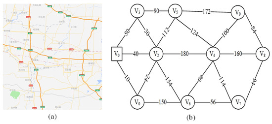
Figure 3. The improved measure function for freshness. (a) The local road network in the flood-stricken area. (b) Abstract map of the local road network in the flood-stricken area.

Table 5. The minimum requirements of the demand point for the freshness of emergency perishable materials.

Demand Point	Material Demand	Minimum Requirements for Freshness
$v_1$	3.5	0.50
$v_2$	3.0	0.50
$v_3$	2.5	0.45
$v_4$	2.0	0.45
$v_5$	2.0	0.50
$v_6$	2.0	0.45
$v_7$	1.5	0.50
$v_8$	1.5	0.45
$v_9$	2.0	0.45

Assuming the freshness period of emergency perishable materials is $t_1=4$, the sub-freshness period is $t_2=16$, the time required for the freshness of emergency perishable materials to drop to zero is $T=20$, and the freshness decay rate during the freshness period is $\beta =0.01$, the freshness measurement function of the emergency perishable materials can be represented by $F\left(t_{0i}\right)=\left\{\begin{array}{c}1-0.01t_{0i},0\le t_{0i}\le 4\hfill \\ 1-0.0025t_{0i}^2,4\le t_{0i}\le 16\hfill \end{array}\right.$. By utilizing the approximate algorithm to solve the model, we obtain the vehicle distribution demand points and distribution routes, which are outlined in Table 6 and Table 7.

Table 6. The distribution route of the vehicle.

Delivery Order	Demand Point	Delivery Distance	Delivery Duration
1	$v_1$	10	0.25
2	$v_2$	34	0.85
3	$v_3$	64	1.6
4	$v_4$	154	3.85
5	$v_5$	238	6.10
6	$v_6$	318	8.10
7	$v_7$	374	9.50
8	$v_8$	468	14.55
9	$v_9$	552	16.65

Table 7. The sum of the freshness of the materials at each demand point.

Delivery Order	Demand Point	The Freshness of Supplies	The Sum of the Freshness
1	$v_1$	0.998	3.491
2	$v_2$	0.992	2.975
3	$v_3$	0.984	2.460
4	$v_4$	0.962	1.923
5	$v_5$	0.907	1.814
6	$v_6$	0.836	1.672
7	$v_7$	0.774	1.162
8	$v_8$	0.471	0.706
9	$v_9$	0.307	0.614

The delivery route of the vehicle is $v_1\to v_2\to v_3\to v_5\to v_4\to v_6\to v_7\to v_8\to v_9$ according to Table 6 and Table 7. However, the freshness of demand point $v_9$ is 0.307, which is less than its minimum freshness requirement of 0.45. Meanwhile, when the vehicle is delivered to the demand point $v_9$, $t_{0i}$ is 16.65 greater than $t_2$, and the material will be completely lost when it reaches $v_9$. Thus, the vehicle stops delivering only after delivering the demand point $v_8$. Finally, the delivery route of the vehicle is $v_1\to v_2\to v_3\to v_5\to v_4\to v_6\to v_7\to v_8$. We compute the sum of the freshness of all demand points as 16.203. The approximate ratio of the designed algorithm is 1.231, which is close to 1. The computed approximate ratio shows that the proposed algorithm works well in practice.

Assuming the freshness period of emergency perishable materials is $t_1=2$, the sub-freshness period is $t_2=5$, the time required for the freshness of emergency perishable materials to drop to zero is $T=10$, and the freshness decay rate during the freshness period is $\beta =0.02$, the freshness measurement function of the emergency perishable materials can be represented by $F\left(t_{0i}\right)=\left\{\begin{array}{c}1-0.02t_{0i},0\le t_{0i}\le 2\hfill \\ 1-0.001t_{0i}^2,2\le t_{0i}\le 8\hfill \end{array}\right.$. By utilizing the approximate algorithm to solve the model, we obtain the vehicle distribution demand points and distribution routes, which are outlined in Table 8 and Table 9.

Table 8. The distribution route of the vehicle.

Delivery Order	Demand Point	Delivery Distance	Delivery Duration
1	$v_1$	10	0.25
2	$v_2$	34	0.85
3	$v_3$	64	1.6
4	$v_4$	154	3.85
5	$v_5$	238	6.10
6	$v_6$	318	8.10
7	$v_7$	374	9.50
8	$v_8$	468	14.55
9	$v_9$	552	16.65

Table 9. The sum of the freshness of the materials at each demand point.

Delivery Order	Demand Point	Freshness of Supplies	Sum of Freshness
1	$v_1$	0.995	3.483
2	$v_2$	0.983	2.949
3	$v_3$	0.968	2.420
4	$v_4$	0.852	1.704
5	$v_5$	0.628	1.256
6	$v_6$	0.344	0.688
7	$v_7$	0.098	0.147
8	$v_8$	0	0
9	$v_9$	0	0

If the delivery time from the distribution center to $v_6,v_7,v_8,v_9$ exceeds $t_2$, the emergency perishable materials will lose their use value, making distribution impractical. Therefore, we have determined the distribution route of the vehicle as $v_1,v_2,v_3,v_5,v_4$ and calculated the freshness ratio of all emergency perishable materials delivered to the demand point. The sum of the freshness ratio is 11.812, and the approximate ratio is 1.685, which is close to 1. This indicates that the algorithm works well in practice again.

5. Conclusions

This paper investigates the optimization of the delivery of emergency perishable supplies with freshness. With the objective of maximizing the sum of the freshness of all demand points, we design a distribution optimization model and a measurement function of the freshness of materials. Meanwhile, we design an approximate algorithm to solve the optimization model. Then, we prove that the time complexity of the designed approximate algorithm is $O\left(n^{2}Olog\left(n\right)\right)$. On this basis, we further analyze the approximate ratio of the designed algorithm. The upper bound of the approximate ratio of the designed algorithm is $\frac{b{Q}^{*}}{a{q}_{*}^1}$, and the lower bound is $\frac{\left[1-\beta t_{*}^1\right]Q^{*}}{\eta }$. Finally, we demonstrate the effectiveness of the proposed model and algorithm with an example.

References

- Sloof, M.; Tijskens, L.M.M.; Wilkinson, E.C. Concepts for modelling the quality of perishable products. Trends Food Sci. Technol. 1996, 7, 165–171. [Google Scholar] [CrossRef]
- Frederickson, G.N.; Hecht, M.S.; Kim, C.E. Approximation algorithms for some routing problems. In Proceedings of the 17th Annual Symposium on Foundations of Computer Science (SFCS 1976), Houston, TX, USA, 25–27 October 1976; Volume 7, pp. 216–227. [Google Scholar]
- Kannan, R.; Karpinski, M. Approximation algorithms for NP-hard problems. Oberwolfach Rep. 2005, 1, 1461–1540. [Google Scholar] [CrossRef]
- Nagarajan, V.; Ravi, R. Approximation algorithms for distance constrained vehicle routing problems. Networks 2012, 59, 209–214. [Google Scholar] [CrossRef]
- Dantzig, G.; Johnson, R.F. Solution of a Large-Scale Traveling-Salesman Problem. J. Oper. Res. Soc. Am. 1954, 2, 393–410. [Google Scholar] [CrossRef]
- Zandkarimkhani, S.; Mina, H.; Biuki, M.; Govindan, K. A chance constrained fuzzy goal programming approach for perishable pharmaceutical supply chain network design. Ann. Oper. Res. 2020, 295, 425–452. [Google Scholar] [CrossRef]
- Liu, Z.; Guo, H.; Zhao, Y.; Hu, B.; Shi, L.; Lang, L.; Huang, B. Research on the optimized route of cold chain logistics transportation of fresh products in context of energy-saving and emission reduction. Math. Biosci. Eng. 2021, 18, 1926–1940. [Google Scholar] [CrossRef]
- Feng, Y.; Liu, Y.K.; Chen, Y. Distributionally robust location–allocation models of distribution centers for fresh products with uncertain demands. Expert Syst. Appl. 2022, 209, 118180. [Google Scholar] [CrossRef]
- Liu, X.; Song, X. Emergency operations scheduling for a blood supply network in disaster reliefs. IFAC-PapersOnLine 2019, 52, 778–783. [Google Scholar] [CrossRef]
- Chen, J.; Dong, M.; Xu, L. A perishable product shipment consolidation model considering freshness-keeping effort. Transp. Res. Part E Logist. Transp. Rev. 2018, 115, 56–86. [Google Scholar] [CrossRef]
- Zhou, Y.; Zou, T.; Liu, C.; Yu, H.; Chen, L.; Su, J. Blood supply chain operation considering lifetime and transshipment under uncertain environment. Appl. Soft Comput. 2021, 106, 107364. [Google Scholar] [CrossRef]
- Zahiri, B.; Jula, P.; Tavakkoli-Moghaddam, R. Design of a pharmaceutical supply chain network under uncertainty considering perishability and substitutability of products. Inf. Sci. 2019, 70, 605–625. [Google Scholar] [CrossRef]
- Rahbari, A.; Nasiri, M.M.; Werner, F.; Musavi, M.; Jolai, F. The vehicle routing and scheduling problem with cross-docking for perishable products under uncertainty: Two robust bi-objective models. Appl. Math. Model. 2019, 70, 605–625. [Google Scholar] [CrossRef]
- Zhang, H.; Cui, Y.; Deng, H.; Cui, S.; Mu, H. An improved genetic algorithm for the optimal distribution of fresh products under uncertain demand. Mathematics 2021, 9, 2233. [Google Scholar] [CrossRef]
- Li, Y.; Lim, M.K.; Tseng, M.L. A green vehicle routing model based on modified particle swarm optimization for cold chain logistics. Ind. Manag. Data Syst. 2019, 119, 473–494. [Google Scholar] [CrossRef]
- Rong, A.; Akkerman, R.; Grunow, M. An optimization approach for managing fresh food quality throughout the supply chain. Int. J. Prod. Econ. 2011, 131, 421–429. [Google Scholar] [CrossRef]
- Jedermann, R.; Praeger, U.; Geyer, M.; Lang, W. Remote quality monitoring in the banana chain. Philos. Trans. R. Soc. A Math. Phys. Eng. Sci. 2014, 372, 20130303. [Google Scholar] [CrossRef]
- Amorim, P.; Almada-Lobo, B. The impact of food perishability issues in the vehicle routing problem. Comput. Ind. Eng. 2014, 67, 223–233. [Google Scholar] [CrossRef]
- Rabbani, M.; Farshbaf-Geranmayeh, A.; Haghjoo, N. Vehicle routing problem with considering multi-middle depots for perishable food delivery. Uncertain Supply Chain. Manag. 2016, 4, 171–182. [Google Scholar] [CrossRef]
- Mercier, S.; Uysal, I. Neural network models for predicting perishable food temperatures along the supply chain. Biosyst. Eng. 2018, 171, 91–100. [Google Scholar] [CrossRef]
- Hsiao, Y.H.; Chen, M.C.; Lu, K.Y.; Chin, C.L. Last-mile distribution planning for fruit-and-vegetable cold chains. Int. J. Logist. Manag. 2018, 29, 862–886. [Google Scholar] [CrossRef]
- Stellingwerf, H.M.; Groeneveld, L.H.; Laporte, G.; Kanellopoulos, A.; Bloemhof, J.M.; Behdani, B. The quality-driven vehicle routing problem: Model and application to a case of cooperative logistics. Int. J. Prod. Econ. 2021, 231, 107849. [Google Scholar] [CrossRef]
Disclaimer/Publisher’s Note: The statements, opinions and data contained in all publications are solely those of the individual author(s) and contributor(s) and not of MDPI and/or the editor(s). MDPI and/or the editor(s) disclaim responsibility for any injury to people or property resulting from any ideas, methods, instructions or products referred to in the content. |
© 2023 by the authors. Licensee MDPI, Basel, Switzerland. This article is an open access article distributed under the terms and conditions of the Creative Commons Attribution (CC BY) license (https://creativecommons.org/licenses/by/4.0/).