
Analytic Study of Coupled Burgers’ Equation


Abstract
:1. Introduction
2. The Homotopy Analysis Method
3. Convergence Analysis
4. Application
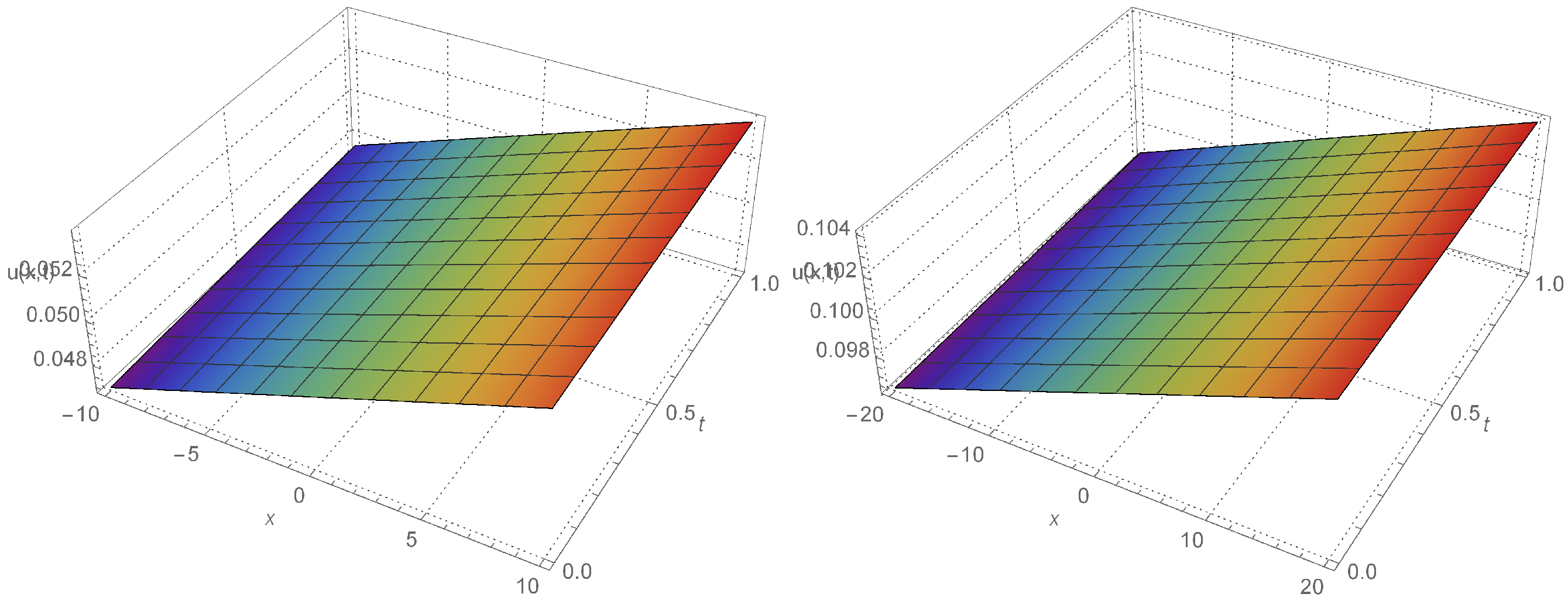
4.1. Test Example 1
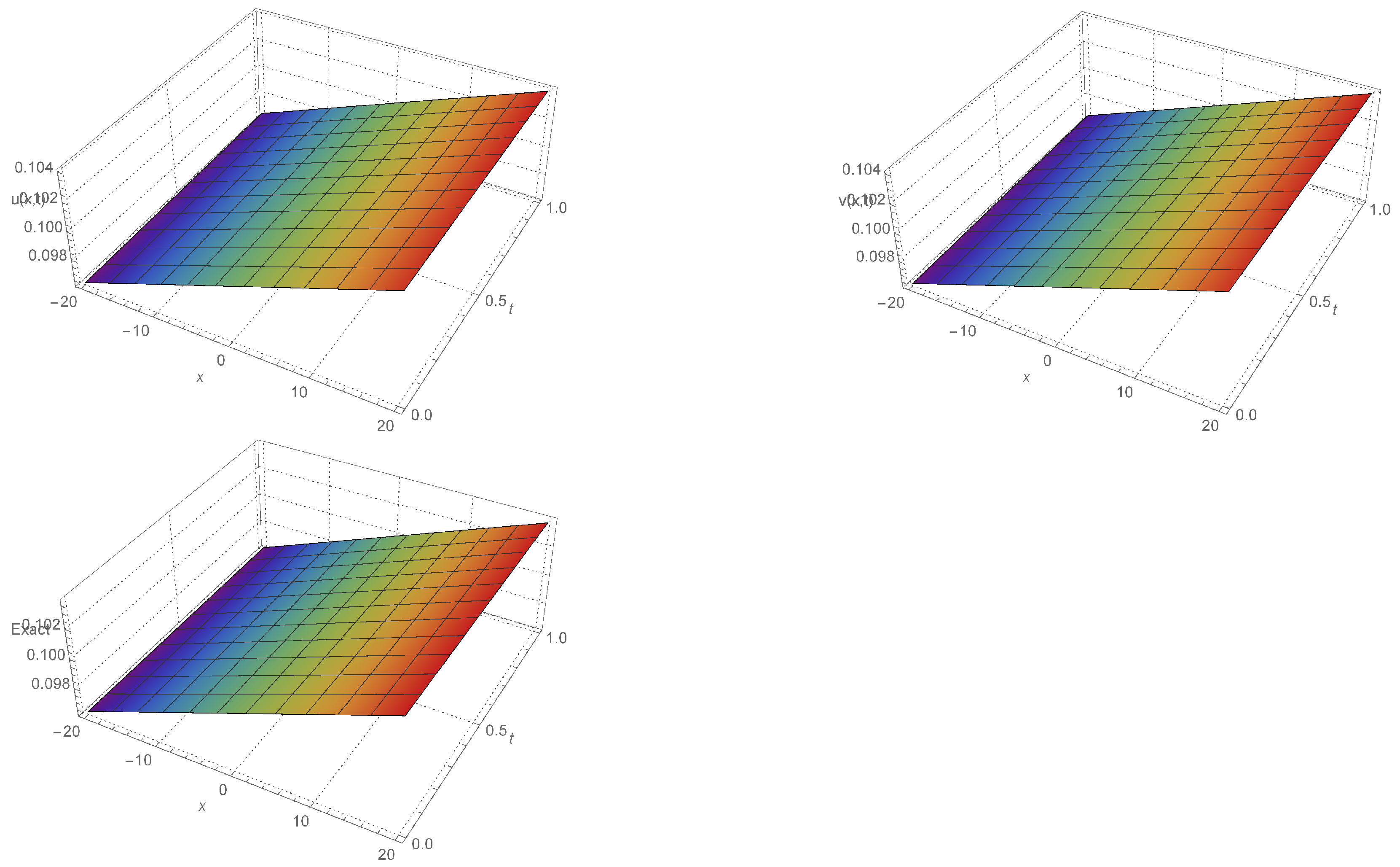
4.2. Test Example 2
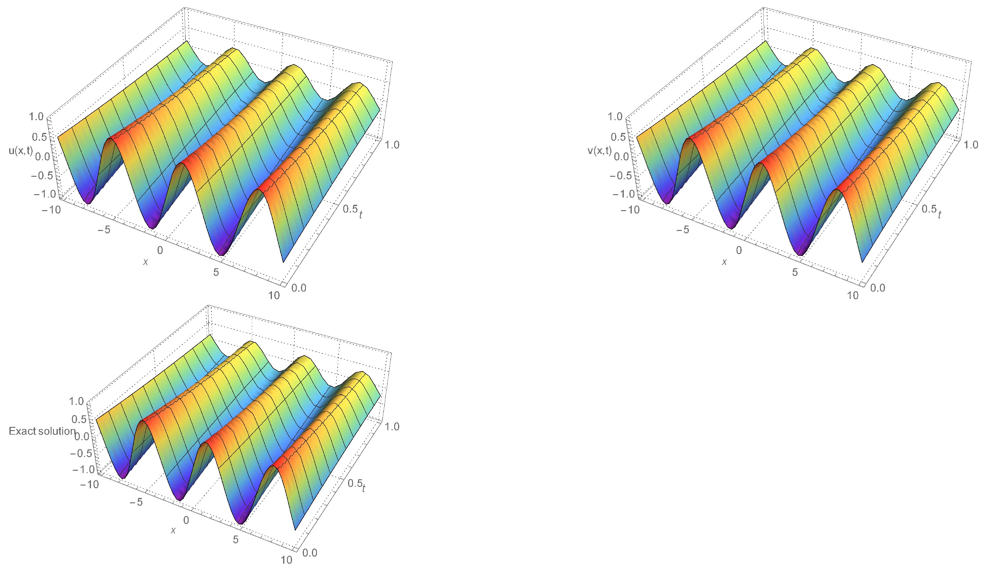
4.3. Test Example 3
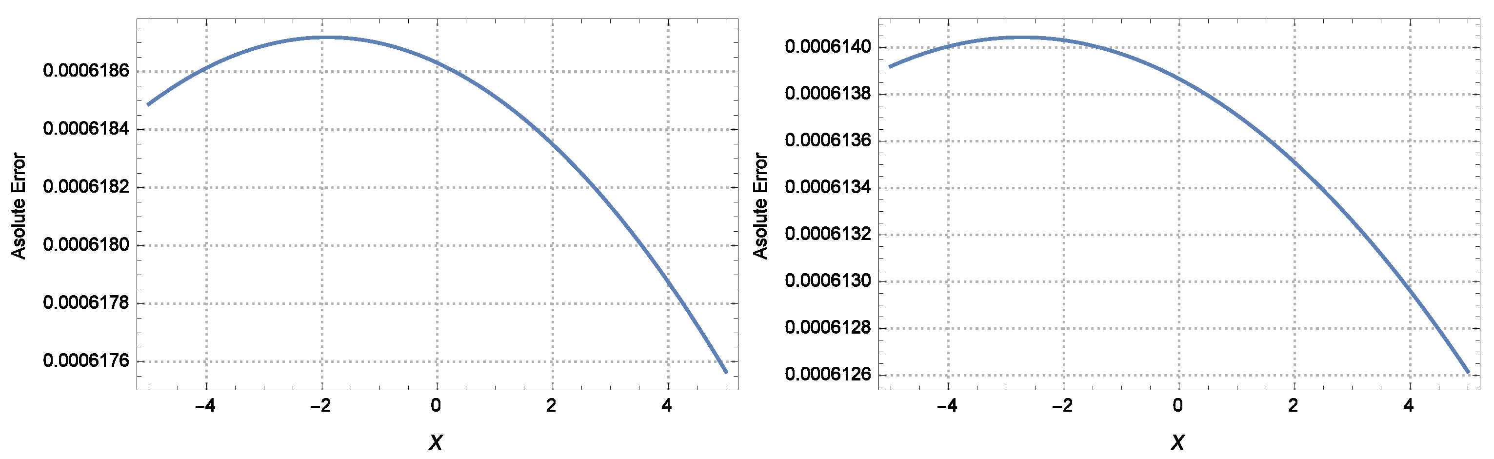
5. Numerical Result and Discussion
6. Conclusions
Author Contributions
Funding
Data Availability Statement
Acknowledgments
Conflicts of Interest
References
- Akbar, M.A.; Ali, N.H.M.; Tanjim, T. Outset of multiple soliton solutions to the nonlinear Schrödinger equation and the coupled Burgers equation. J. Phys. Commun. 2019, 3, 095013. [Google Scholar] [CrossRef]
- Aziz, A.; Khani, F.; Darvishi, M.T. Homotopy Analysis Method for Variable Thermal Conductivity Heat Flux Gage with Edge Contact Resistance. Verl. Z. Naturforschung 2010, 8, 119. [Google Scholar] [CrossRef]
- Ahmad, H.; Khan, T.A.; Cesarano, C. Numerical solutions of coupled Burgers’ equations. Axioms 2019, 8, 119. [Google Scholar] [CrossRef]
- Khater, A.; Temsah, R.; Hassan, M. A Chebyshev spectral collocation method for solving Burgers’-type equations. J. Comput. Appl. Math. 2008, 222, 333–350. [Google Scholar] [CrossRef]
- Rashid, A.; Abbas, M.; Ismail, A.I.M.; Majid, A.A. Numerical solution of the coupled viscous Burgers equations by Chebyshev–Legendre Pseudo-Spectral method. Appl. Math. Comput. 2014, 245, 372–381. [Google Scholar] [CrossRef]
- Ahmad, H. Variational Iteration Algorithm-I with an Auxiliary Parameter for Solving Fokker–Planck Equation. Earthline J. Math. Sci. 2019, 2, 29–37. [Google Scholar] [CrossRef]
- Darvishi, M.T.; Kheybari, S.; Khani, F. A numerical solution of the Korteweg-de Vries equation by pseudospectral method using Darvishi’s preconditionings. Appl. Math. Comput. 2006, 1, 98–105. [Google Scholar] [CrossRef]
- Liao, S.J. The Proposed Homotopy Analysis Technique for the Solution of Nonlinear Problems. Ph.D. Thesis, Shanghai Jiao Tong University, Shanghai, China, 1992. [Google Scholar]
- Liao, S. Notes on the homotopy analysis method: Some definitions and theorems. Commun. Nonlinear Sci. Numer. Simul. 2009, 14, 983–997. [Google Scholar] [CrossRef]
- Liao, S. Homotopy Analysis Method in Non-Linear Differential Equations, 3rd ed.; Springer: Berlin/Heidelberg, Germany; Dordrecht, The Netherlands; London, UK; New York, NY, USA, 2012. [Google Scholar]
- Alomari, A.K.; Drabseh, G.A.; Al-Jamal, M.F.; AlBadarneh, R.B. Numerical simulation for fractional phi-4 equation using homotopy Sumudu approach. Int. J. Simul. Process. Model. 2021, 16, 26–33. [Google Scholar] [CrossRef]
- Shather, A.H.; Jameel, A.F.; Anakira, N.R.; Alomari, A.K.; Saaban, A. Homotopy analysis method approximate solution for fuzzy pantograph equation. Int. J. Comput. Sci. Math. 2021, 14, 286–300. [Google Scholar] [CrossRef]
- Hashim, D.J.; Jameel, A.F.; YuanYing, T.; Alomari, A.K.; Anakira, N.R. Optimal homotopy asymptotic method for solving several models of first-order fuzzy fractional IVPs. Alex. Eng. J. 2022, 61, 4931–4943. [Google Scholar] [CrossRef]
- Aljhani, S.; Noorani, M.S.M.; Saad, K.M.; Alomari, A.K. Numerical Solutions of Certain New Models of the Time-Fractional Gray-Scott. J. Funct. Spaces 2021, 2021, 2544688. [Google Scholar] [CrossRef]
- Liao, S. An optimal homotopy-analysis approach for strongly nonlinear differential equations. Commun. Nonlinear Sci. Numer. Simul. 2010, 15, 2003–2016. [Google Scholar] [CrossRef]
- Saad, K.M.; AL-Shareef, E.H.; Alomari, A.K.; Baleanu, D.; Gómez-Aguilar, J.F. On exact solutions for time-fractional Korteweg-de Vries and Korteweg-de Vries-Burger’s equations using homotopy analysis transform method. Chin. J. Phys. 2020, 63, 149–162. [Google Scholar] [CrossRef]


| x | t | Exact | HAM | Absolute Error |
|---|---|---|---|---|
| −10 | ||||
| 1 | ||||
| 5 | ||||
| 10 | ||||
| 1 | ||||
| 5 | ||||
| 10 | ||||
| 0 | ||||
| 1 | ||||
| 5 | ||||
| 10 | ||||
| 5 | ||||
| 1 | ||||
| 5 | ||||
| 10 | ||||
| 10 | ||||
| 1 | ||||
| 5 | ||||
| 10 |
| x | t | Exact | HAM | Absolute Error |
|---|---|---|---|---|
| −10 | ||||
| 1 | ||||
| 5 | ||||
| 10 | ||||
| 1 | ||||
| 5 | ||||
| 10 | ||||
| 0 | ||||
| 1 | ||||
| 5 | ||||
| 10 | ||||
| 5 | ||||
| 1 | ||||
| 5 | ||||
| 10 | ||||
| 10 | ||||
| 1 | ||||
| 5 | ||||
| 10 |
| x | t | Exact | HAM u | Absolute Error u | HAM v | Absolute Error v |
|---|---|---|---|---|---|---|
| −10 | ||||||
| 1 | ||||||
| 5 | ||||||
| 10 | ||||||
| −5 | ||||||
| 1 | ||||||
| 5 | ||||||
| 10 | ||||||
| 0 | ||||||
| 1 | ||||||
| 5 | ||||||
| 10 | ||||||
| 5 | ||||||
| 1 | ||||||
| 5 | ||||||
| 10 | ||||||
| 10 | ||||||
| 1 | ||||||
| 5 | ||||||
| 10 |
Disclaimer/Publisher’s Note: The statements, opinions and data contained in all publications are solely those of the individual author(s) and contributor(s) and not of MDPI and/or the editor(s). MDPI and/or the editor(s) disclaim responsibility for any injury to people or property resulting from any ideas, methods, instructions or products referred to in the content. |
© 2023 by the authors. Licensee MDPI, Basel, Switzerland. This article is an open access article distributed under the terms and conditions of the Creative Commons Attribution (CC BY) license (https://creativecommons.org/licenses/by/4.0/).
Share and Cite
Cesarano, C.; Massoun, Y.; Said, A.; Talbi, M.E. Analytic Study of Coupled Burgers’ Equation. Mathematics 2023, 11, 2071. https://doi.org/10.3390/math11092071
Cesarano C, Massoun Y, Said A, Talbi ME. Analytic Study of Coupled Burgers’ Equation. Mathematics. 2023; 11(9):2071. https://doi.org/10.3390/math11092071
Chicago/Turabian StyleCesarano, Clemente, Youssouf Massoun, Abderrezak Said, and Mohamed Elamine Talbi. 2023. "Analytic Study of Coupled Burgers’ Equation" Mathematics 11, no. 9: 2071. https://doi.org/10.3390/math11092071