Abstract
The aim of this contribution is to propose a numerical scheme for solving linear and nonlinear boundary value problems. The scheme is implicit and it is constructed on three grid points. The stability of the proposed implicit scheme is provided. In addition to this, a mathematical model for heat and mass transfer using induced magnetic field (IMF) is modified. Furthermore, this model is transformed into boundary value problems by employing similarity transformations. The dimensionless model of boundary value problems is solved using the proposed numerical scheme. The scheme is applied with a combination of a shooting approach and an iterative method. From the obtained results, it can be seen that velocity profile declines with enhancing Weissenberg number. The results are also compared with those given in past research. In addition to this, a neural network approach is applied that is based on the input and outputs of the considered model with specified values of parameters.
MSC:
65L10
1. Introduction
Electrically conducted fluid flow, with consideration of magnetic field, has applications in different fields such as geophysics, astrophysics, MHD natural convection flow, heat exchangers and electronics. There exists a physical phenomenon in which flow of fluid is controlled by the magnetic field, such as plasma theory and MHD coolants and generators. The effect of an induced magnetic field on boundary layer flow has not been discussed by various researchers, but some researchers shown interest in the several scientific and technological phenomena in induced magnetic fields. Furthermore, it can be seen that the field of plasma has significant use for an induced magnetic field. The induced magnetic field has applications in earth surface geothermal examination, sunspots, cosmic rays and under earth surface flow.
In [1], induced magnetic fields have been considered with ferrofluid flow over the flat plate. The plate was a semi-infinite plate, and the flow was generated through the sudden jerk of the plate. The Navier–Stokes equation, with a combination of heat equations, have been considered for modelling the flow under the effect of IMF. In most of the studies [2,3,4], the governing equations have been expressed in the form of partial differential equations (PDEs) and, later on, these PDEs have been reduced to ODEs using some transformations. Mostly, two dimensional fluid flow [5,6,7] has been considered under different effects. In the existing literature, two different types of methods have been adopted to study the effect of different forces on boundary layer flows. Sometimes [8,9] different types of nanoparticles in the base fluid have been added to enhance heat transfer. For nanofluid, there exists another mathematical model called a Buongiorno’s nanofluid model [10,11,12] that gives a set of partial differential equations under the effect of heat and mass transfers. This Buongornoue model is studied by some authors to model the flow phenomenon that adds the mass transfer equation to a combination of other equations. The induced magnetic flux has been utilized on Oldroyd 4-constant nanofluid [13]. Non-linear partial differential equations have been simplified by the use of a low finite Reynolds number. The exact solution of the considered differential equations has been found. It was found that by rising magnetic Reynolds number and electric field, magnetic force function escalated. The study of convective Casson fluid under the effect of exponential heat source and induced magnetic field has been given in [14].
In some fields, new ways to escalate heat transfer rate as a thermal system are required for high thermal performance. Heat exchangers transfer heat between two objects and these are found in petroleum processing, air conditioners and pharmaceuticals. The first time Tuckerman and Pease [15] utilized a microchannel as heat exchanger, from the given results it was observed that thermal resistance was decayed by a high aspect ratio. In a micro channel, heat transfer between two various liquids has been studied in [14]. The results were calculated using different approaches and it was found that Akbari-Ganji’s method (AGM) confirmed the accuracy of results which were obtained by AGM. The boundary layer flow has applications in glass fiber and paper production, in material manufacturing by an extrusion process and in industrial applications including polymer sheets. In the mentioned fields, the desired characteristic depends on the cooling and stretching within the physical aspects.
For solving any mathematical model of differential equations, it is necessary to apply some analytical or numerical scheme. In the literature, there exist finite difference methods to handle linear and non-linear differential equations. Among these, a generalized finite difference method has been applied [16] for solving hyperbolic two-phase coupling problems. To solve discretized equations, a nonlinear solver based on Newton’s method has been employed. Due to its constructing procedure, the proposed method ensures low computational cost and reduces the dissipation error of the calculation. Several numerical test cases have been carried out for analyzing accuracy and computational performance. For the solution of two-phase porous flow equations [17], a newly developed generalized finite difference method has been applied. Instead of using mesh generation, the computational domain has been flexibly discretized using a node cloud. The non-linear solver based on Newton’s method has been applied. The upwind generalized finite difference method with a combination of fully implicit non-linear solvers and related analysis might be a critical reference for constructing a meshless numerical simulator for problems of porous flow. Another finite difference method for space discretization, called a Mimetic finite difference method, has been employed in [18]. On distorted meshes, it achieved second-order accuracy and local mass conservation. A comparison was made with past research and the employed methods converged quickly. Since there exist numerous schemes in the literature, among them some were unconditionally stable. Therefore, any step size in time and space can be used. Thus, there is no restriction imposed on the step size when an unconditionally stable scheme is adopted. In this contribution, a scheme is proposed that is unconditionally stable in partial differential equations. The scheme is applied in this contribution to find a solution for ordinary differential equations. More work on boundary layer flow can be seen in [19,20] and references therein.
The impact dynamics of a ferrofluid droplet on PDMS substrate have been reported in [21] in the presence of a non-uniform magnetic field. It was shown that the equilibrium shaper of the ferrofluid droplet was effected by the viscous, magnetic, interfacial energies and inertia. In dictating the droplet’s equilibrium shape, the role of various dynamic forces has been demonstrated. The transportation phenomenon of heat in nanofluid flow with entropy generation has been investigated in [22] under the combined effects of electrical forcing and pressure gradient. The influence of the transportation of heat through the channel walls was also considered. The optimum value of the geometrical parameter viz. the thermophysical parameter, the channel wall thickness, the Biot number, the thermal conductivity and the modified Peclet number were obtained by the non-trivial interplay among irreversibility. The entropy generation characteristic and natural convective heat transfer in a wavy solar power plant were investigated in [23]. The finite element method was considered to solve the fluid phenomenon. It was concluded that the strength of recirculation developed in the flow field was declined by the presence of a wavy wall and nanoparticles. The average Nusselt number was raised by an escalation of nano-particle volume fraction and an amplitude of the wavy wall. The study of combined convective heat transfer for hybrid nanofluid flow in an open trapezoidal enclosure under the effects of magnetohydrodynamics and radiation is given in [24]. The enclosure contained a horizontal wall and two diagonal side walls. The embedded boundary approach was considered to model the inclined side of an enclosure. Rosseland approximation was adopted to handle thermal radiation terms in an energy equation. The result showed that, at the bottom wall, the magnitude of total heat transfer rate was maximum for the case when no magnetic force is applied.
2. Numerical Scheme
For proposing a numerical scheme for finding a solution for differential equations, consider a differential equation with initial condition such as
where is a constant.
The general form of a difference scheme is given as
where and are constants to be determined later.
For finding and , consider the Taylor series expansion for , and as:
Substituting (3)–(5) into Equation (2) yields:
Equating coefficients of and in Equation (6) yields:
Solving Equations (7) and (8) gives the values of and as:
Therefore, the proposed scheme can be written as:
Rewrite Equation (10) as:
3. Stability Analysis
For finding the stability condition of the proposed scheme, consider the following linear equation:
Applying the proposed scheme on Equation (12) gives:
Rewrite Equation (13) as:
The characteristic polynomial is:
The zeros of (15) can be written as:
Thus, the region of absolute stability is given as:
For finding the stability conditions for system of equations, consider the following vector-matrix equation
where is a vector and is a matrix.
The proposed scheme with the Gauss–Seidel iterative method for Equation (18) is given as:
Consider the transformations for Equation (19) as
where .
Substituting transformations (20) into Equation (19) gives:
Dividing both sides of Equation (21) by yields:
Rewrite Equation (22) as
where denotes the identity matrix.
The amplification factor is given as
where denotes the maximum eigenvalue of .
4. Problem Formulation
Consider the incompressible, laminar, two dimensional, steady, Williamson fluid flow over a moving sheet. The velocity of a moving sheet is denoted by . The sudden movement of the sheet generates the flow. Let -axis and -axis be, respectively, taken along the sheet and perpendicular to the sheet. The flow is considered with a magnetic field with a strength of . The effect of the induced magnetic field (IMF) is considered with the assumption of a large magnetic Reynolds number. The horizontal component of IMF in -direction is denoted by . Let to be a normal component of the induced magnetic field and at the sheet. The governing equations of the flow can be written as [1,2,3,4]
subject to the boundary conditions
The study of Buongiorno’s nanofluid is considered for this contribution, so the second and third terms in the energy Equation (29), and the first and second terms in Equation (31), are part of an adopted mathematical model of nanofluid flow. The last terms in Equations (29) and (30) are used for showing the effects of a viscous dissipation and a chemical reaction, respectively. The second term in Equation (27) shows the effect of non-Newtonian Williamson fluid, or comes from the tensor of the Williamson fluid. The geometry of the problem is given in Figure 1.
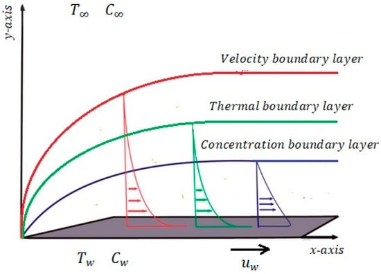
Figure 1.
Geometry of the problem.
For making Equations (25)–(31) dimensionless, the following transformations are considered:
Applying transformations to (25)–(31) as
subject to the dimensionless boundary conditions
The quantities of physical interest skin friction coefficient, and local Nusselt and Sherwood numbers are defined in the following manner:
where , and .
Using transformations in (30) in Equations (36)–(38) obtains:
5. Results and Discussions
The stability of a numerical scheme is one of the factors that is used to check convergence of the numerical scheme. Since it is second-order accurate, it is consistent. The consistency of the proposed numerical scheme can be proved by applying a Taylor series for some terms of Equation (13). The scheme is a multi-step scheme that has one drawback in that it requires a solution found at first time level. So, in order to obtain the solution at the first time level, either some other solution method or some supposed solution can be considered. Thus, for this contribution, the forward Euler method is adopted to find a solution at first time level. Furthermore, since the proposed scheme is an implicit one, so in order to handle the implicit difference equations that are obtained by applying the proposed scheme on given differential equations, additionally an iterative method is considered. The adopted iterative method requires one initial guess to start the solution procedure. It requires some stopping criteria to stop the computational procedure. For the computations given in this contribution, a maximum of all the norms is adopted to apply the stopping criteria. The iterative technique will be stopped if the maximum of all norms for the difference of two solutions computed on two consecutive iterations is less than some given tolerance. When the iterative method is stopped, the solution obtained at final iteration is considered for simulations. The numerical scheme considered in this contribution can be applied to solve first-order ODEs or higher-order initial value problems. A shooting strategy is employed in order to apply the proposed scheme on second- or third-order boundary value problems. For solving equations obtained by applying a shooting method, the Matlab solver fsolve is employed and the proposed scheme is utilized to solve differential equations with given or assumed initial conditions. The second and third-order boundary value problems are reduced to first-order ODEs with given or assumed initial conditions for the set of first-order differential equations obtained from governing equations of flow phenomenon.
Figure 2 shows the velocity profile by variation of the Weissenberg number. By looking at Figure 2, it can be observed that velocity profile decreases by rising Weissenberg number. Figure 3 deliberates the influence of magnetic parameter and reciprocal of the magnetic Prandtl number on velocity profile and the horizontal component of an induced magnetic field, respectively. Velocity profile declines and horizontal component of induced magnetic field has a dual behaviour by rising the values of magnetic parameters and reciprocal of magnetic Parndtl number, respectively. The decline in velocity profile due to rising magnetic parameters is a consequence of the enhancement of viscosity that resists the velocity of fluid. Figure 4 displays the effect of the Eckert number and Prandtl number on temperature profile. Temperature profile grows and declines respectively by increasing values of Eckert and Prandtl numbers. The growth in the temperature profile is the consequence of growing internal friction between particles due to the increase in the Eckert number. The decay in the temperature profile is the result of the decreasing thermal conductivity of the fluid and this happens because thermal conductivity and thermal diffusivity are in direct proportion, and thermal diffusivity and Prandtl number are in inverse proportion. Figure 5 displays the influence of thermophoresis parameter and Brownian motion parameter on temperature profile. Temperature profile escalates with rising thermophoresis and Brownian motion parameters. Since the increment in thermophoresis parameter produces an enhancement of the cycle in which hot particles of fluid shift from the plate to its vicinity and cooler particles move towards the plate, this results in a growth in temperature profile. Furthermore, due to the increment in Brownian motion parameters, particles of fluid scatter in different locations, and so temperature profile grows. Figure 6 portrays the influence of the Schmidt number and reaction rate parameter on concentration profile. It can be seen that concentration profile declines with rising Schmidt number and reaction rate parameter. Since Schmidt number and mass diffusivity are in direct proportion, one therefore increases or decreases with respective increase or decrease of the other, and thus the concentration profile declines due to the decay in mass diffusivity.
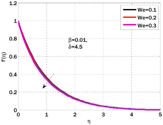
Figure 2.
Effect of Weissenberg number on velocity profile using
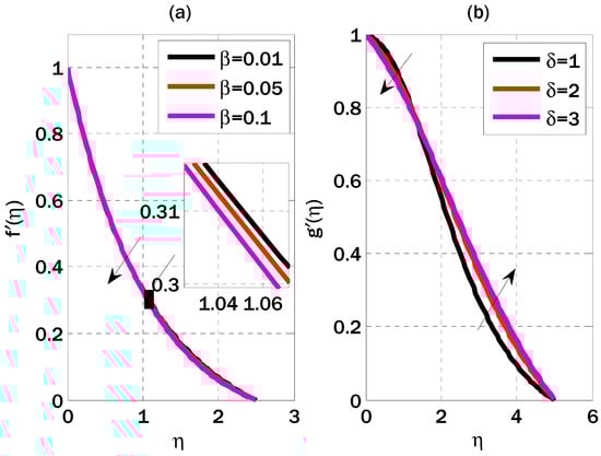
Figure 3.
Effect of magnetic parameter and reciprocal of magnetic Prandtl number on velocity profile and horizontal component of IMF using
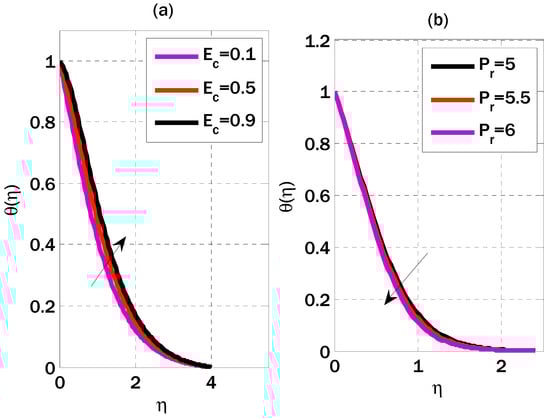
Figure 4.
Effect of Eckert number and Prandtl number on temperature profile using
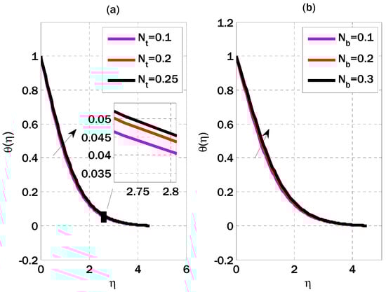
Figure 5.
Effect of thermophoresis and Brownian motion parameters on temperature profile using
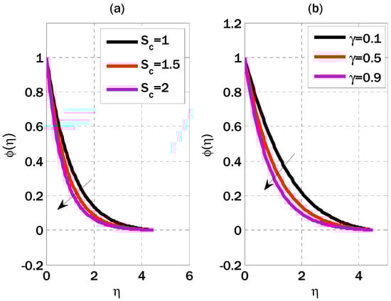
Figure 6.
Effect of thermophoresis and Brownian motion parameters on concentration profile using
The numerical values for parameters depend on the convergence of the proposed scheme. The numerical scheme will converge if it satisfies the given criteria of stopping the iterative procedure. Therefore, those particular values of the parameters can be chosen and the effect of those parameters on velocity, temperature and concentration profiles can be shown. The choice of the numerical values for parameters may depend on the physical aspect of flow phenomenon or any random value(s) can be chosen that will be valid from mathematical point of view. The proposed scheme can be applied to any type of high-order ODE to find its solution. The considered approach is a shooting that finds missing assumed initial conditions by using given boundary conditions. The method can be more simple if a set of initial value problems is given to solve. Therefore, in this case, there is no need to adopt any shooting strategy. Furthermore, the non-Newtonian behavior affects the thickness of the boundary layer. Therefore, this is the main difference between Newtonian and non-Newtonian fluids. If effects of Newtonian and non-Newtonian fluids are considered for boundary layer flow(s), the asymptotic behaviour of contained profiles must be obtained. So, the only difference is thickness of a boundary layer that depends on the inclusion of Newtonian or non-Newtonain fluid.
This study is also concerned with the application of the Levenberg–Marquardt back propagation algorithm for input and outputs of velocity, temperature and concentration profiles. A two-layer feed forward network is designed with sigmoid hidden neurons and linear output neurons. If there is enough memory, the Levenberg–Marquardth back propagation algorithm is applied using the Matlab tool kit nftool and, for memory issues, a scaled conjugate back propagation is adopted. In total, 70% of the whole data is used for training, 15% is used for validation and 15% is used for testing. By default, 10 hidden neurons are used. Figure 7, Figure 8 and Figure 9 show the validation performance for three networks corresponding to velocity, temperature and concentration profiles. Figure 10, Figure 11 and Figure 12 show the error histograms with zero error, showing the minimum error between output and target values. Figure 13, Figure 14 and Figure 15 show the regression plots for three networks of velocity, temperature and concentration profiles.
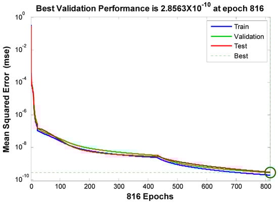
Figure 7.
Validation performance for velocity profile using
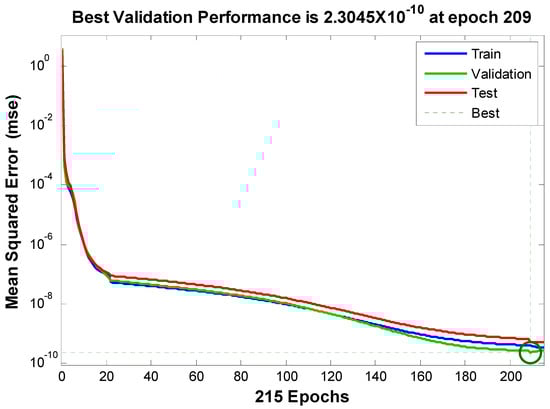
Figure 8.
Validation performance for temperature profile using
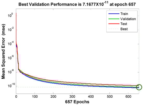
Figure 9.
Validation performance for concentration profile using
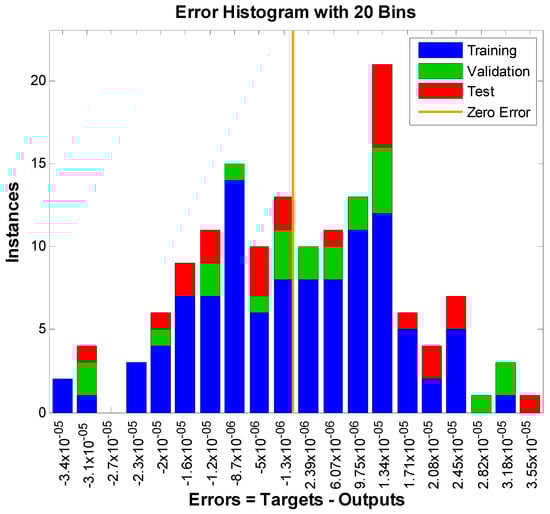
Figure 10.
Error histogram for velocity profile using
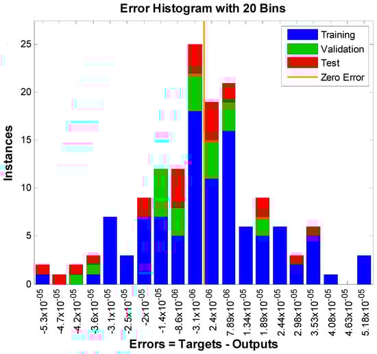
Figure 11.
Error histogram for temperature profile using
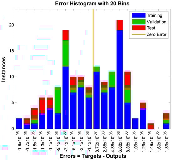
Figure 12.
Error histogram for concentration profile using
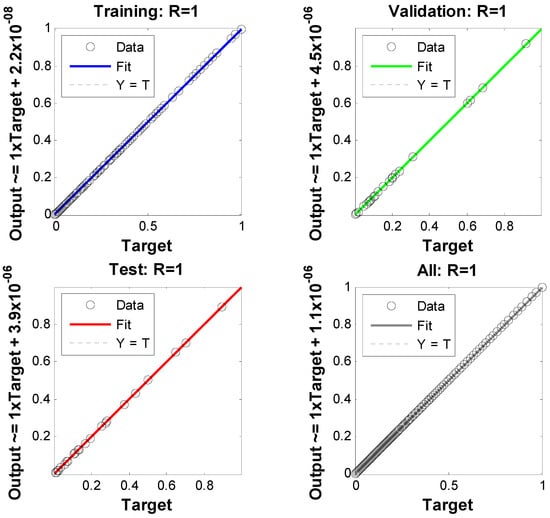
Figure 13.
Regression plot for velocity profile using
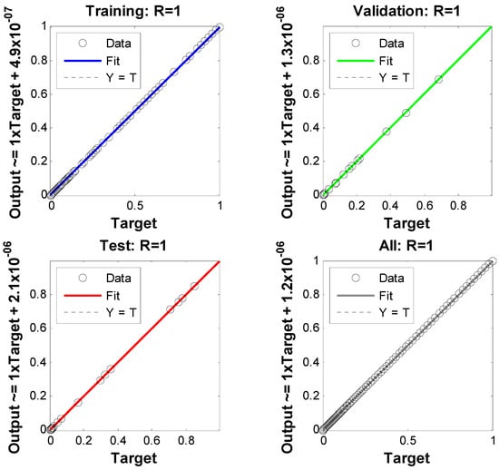
Figure 14.
Regression plot for temperature profile using
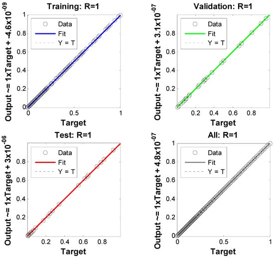
Figure 15.
Regression plot for concentration profile using
The list of numerical values for local Nusselt number by varying Prandtl number is given in Table 1. Table 2 demonstrates a list of numerical values for the quantity of physical interest skin friction coefficient by varying magnetic parameter, reciprocal of magnetic parameter and Weissenberg number. Table 2 shows that skin friction coefficient declines with enhancing magnetic parameter and Weissenberg number, and that it stays the same for incrementing reciprocal of magnetic Prandtl number. The variation of thermophoresis parameter, Brownian motion parameter and Eckert number on local Nusselt number is presented in Table 3. The local Nusselt number declines with varying thermophoresis and Brownian motion parameter, and it rises with enhancing Eckert number. The variation of thermophoresis parameter, Brownian motion parameter and reaction rate parameter on local Sherwood number is demonstrated in Table 4. Local Sherwood number declines with improving thermophoresis parameter, and it develops with accelerating Brownian motion parameter and reaction rate parameter.

Table 1.
Comparison of some results obtained by the proposed scheme and those given in past research using .
Table 2.
Numerical values of skin friction coefficient.
Table 3.
Numerical values of local Nusselt number using
Table 4.
Numerical values of local Sherwood number using
6. Conclusions
A second-order accurate scheme has been proposed to solve systems of ODEs. The stability of the proposed scheme for linear ODEs, as well as for linearized systems of ODEs, has been provided. The scheme was constructed on three grid points or time levels. The scheme was constructed for first-order differential equations, but the considered system of boundary value problems has been tackled using the scheme. In doing this, a shooting approach was been adopted so that the scheme was capable of solving any set of linear and nonlinear second- and third-order ODEs with boundary conditions. The problem that was solved by the scheme was a boundary layer flow problem over the moving sheet using the effect of an induced magnetic field that was handled by the proposed scheme. The concluding points can be expressed as:
- It has been seen that velocity profile decayed with an enhancing of Weissenberg number;
- The horizontal component of velocity has a dual behavior with rising reciprocal of magnetic Prandtl number;
- The temperature profile declined and raised with enhancing Prandtl number and Eckert number, respectively.
Author Contributions
Conceptualization, Y.N.; Methodology, H.J.A.S.; Software, Y.N.; Validation, Y.N.; Formal analysis, Y.N. and A.A.A.G.; Investigation, A.A.A.G.; Resources, A.A.A.G.; Writing—original draft, Y.N.; Writing—review & editing, H.J.A.S. and A.A.A.G.; Project administration, H.J.A.S.; Funding acquisition, H.J.A.S. All authors have read and agreed to the published version of the manuscript.
Funding
This work was supported by the Deanship of Scientific Research, Vice Presidency for Graduate Studies and Scientific Research, King Faisal University, Saudi Arabia [Grant No. 3232].
Data Availability Statement
There is no data available on any website or any source.
Conflicts of Interest
The authors declare no conflict of interest.
Nomenclature
| Horizontal components of velocity | Electrical conductivity of the fluid | ||
| Cartesian co-ordinate | Temperature of fluid | ||
| Kinematic viscosity | Temperature of fluid at the wall | ||
| Density of fluid | Ambient temperature of the fluid | ||
| Concentration of fluid | Concentration on the wall | ||
| Brownian diffusion coefficient | Ambient concentration | ||
| Specific heat capacity | Thermophoresis coefficient | ||
| Horizontal component of induced magnetic field | Vertical component of induced magnetic field | ||
| Reaction rate | Thermal diffusivity | ||
| Reaction rate parameter | Dynamic viscosity | ||
| Time constant (s) | Effective heat capacity of fluid | ||
| Magnetic diffusivity | Eckert number | ||
| Prandtl number | Thermophoresis variable | ||
| Brownian motion variable | Schmidt number | ||
| Magnetic parameter | Weissenberg number | ||
| Reciprocal of magnetic Prandtl number |
References
- Iqbal, M.S.; Malik, F.; Mustafa, I.; Khan, I.; Ghaffari, A.; Riaz, A.; Nisar, K. Impact of induced magnetic field on thermal enhancement in gravity driven Fe3O4 ferrofluid flow through vertical non-isothermal surface. Results Phys. 2020, 19, 103472. [Google Scholar] [CrossRef]
- Kumar, D. Radiation effect on magnetohydrodynamic flow with induced magnetic field and Newtonian heating/cooling: An analytic approach. Propuls. Power Res. 2021, 10, 303–313. [Google Scholar] [CrossRef]
- Khan, U.; Zaib, A.; Ishak, A.; Waini, I.; Pop, I.; Elattar, S.; Abed, A.M. Stagnation point flow of a water-based graphene-oxide over a stretching/shrinking sheet under an induced magnetic field with homogeneous-heterogeneous chemical reaction. J. Magn. Magn. Mater. 2023, 565, 170287. [Google Scholar] [CrossRef]
- Hayat, T.; Rashid, M.; Khan, M.I.; Alsaedi, A. Melting heat transfer and induced magnetic field effects on flow of water based nanofluid over a rotating disk with variable thickness. Results Phys. 2018, 9, 1618–1630. [Google Scholar] [CrossRef]
- Hayat, T.; Razaq, A.; Khan, S.A.; Alsaedi, A. Radiative flow of rheological material considering heat generation by stretchable cylinder. Case Stud. Therm. Eng. 2023, 44, 102837. [Google Scholar] [CrossRef]
- Khan, S.A.; Hayat, T.; Alsaedi, A. Entropy generation in chemically reactive flow of Reiner-Rivlin liquid conveying tiny particles considering thermal radiation. Alex. Eng. J. 2023, 66, 257–268. [Google Scholar] [CrossRef]
- Hayat, T.; Fatima, A.; Khan, S.A.; Alsaedi, A. Thermo-diffusion and diffusion thermo analysis for Darcy Forchheimer flow with entropy generation. Ain Shams Eng. J. 2022, 13, 101530. [Google Scholar] [CrossRef]
- Alsaedi, A.; Muhammad, K.; Hayat, T. Numerical study of MHD hybrid nanofluid flow between two coaxial cylinders. Alex. Eng. J. 2022, 61, 8355–8362. [Google Scholar] [CrossRef]
- Muhammad, K.H.; Hayat, T.; Momani, S.; Asghar, S. FDM analysis for squeezed flow of hybrid nanofluid in presence of Cattaneo-Christov (C-C) heat flux and convective boundary condition. Alex. Eng. J. 2022, 61, 4719–4727. [Google Scholar] [CrossRef]
- Chu, Y.-M.; Al-Khaled, K.; Khan, N.; Khan, M.I.; Khan, S.U.; Hashmi, M.S.; Iqbal, M.A.; Tlili, I. Study of Buongiorno’s nanofluid model for flow due to stretching disks in presence of gyrotactic microorganisms. Ain Shams Eng. J. 2021, 12, 3975–3985. [Google Scholar] [CrossRef]
- Alblawi, A.; Malik, M.Y.; Nadeem, S.; Abbas, N. Buongiorno’s Nanofluid Model over a Curved Exponentially Stretching Surface. Processes 2019, 7, 665. [Google Scholar] [CrossRef]
- Khatun, S.; Nasrin, R. Numerical Modeling Of Buongiorno’s Nanofluid On Free Convection: Thermophoresis And Brownian Effects. J. Nav. Archit. Mar. Eng. 2021, 18, 217–239. [Google Scholar] [CrossRef]
- Akram, S.; Athar, M.; Saeed, K.; Razia, A.; Muhammad, T.; Hussain, A. Hybrid double-diffusivity convection and induced magnetic field effects on peristaltic waves of Oldroyd 4-constant nanofluids in non-uniform channel. Alex. Eng. J. 2023, 65, 785–796. [Google Scholar] [CrossRef]
- Hasibi, A.; Gholami, A.; Asadi, Z.; Ganji, D.D. Importance of induced magnetic field and exponential heat source on convective flow of Casson fluid in a micro-channel via AGM. Theor. Appl. Mech. Lett. 2022, 12, 100342. [Google Scholar] [CrossRef]
- Tuckerman, D.B.; Pease, R.F.W. High performance heat sinking for VLSI. IEEE Electron. Device Lett. 1981, 2, 126–129. [Google Scholar] [CrossRef]
- Liu, Y.; Rao, X.; Zhao, H.; Zhan, W.; Xu, Y.; Liu, Y. Generalized finite difference method based meshless analysis for coupled two-phase porous flow and geomechanics. Eng. Anal. Bound. Elem. 2023, 146, 184–203. [Google Scholar] [CrossRef]
- Rao, X.; Liu, Y.; Zhao, H. An upwind generalized finite difference method for meshless solution of two-phase porous flow equations. Eng. Anal. Bound. Elem. 2022, 137, 105–118. [Google Scholar] [CrossRef]
- Cocoon, E.T.; Moulton, D.; Kikinzon, E.; Berndt, M.; Manzini, G.; Garimella, R.; Lipnikov, K.; Painter, S.L. Coupling surface flow and subsurface flow in complex soil structures using mimetic finite differences. Adv. Water Resour. 2020, 144, 103701. [Google Scholar] [CrossRef]
- Khan, W.A.; Pop, I. Boundary layer flow of a nanofluid past a stretching sheet. Int. J. Heat Mass Tran. 2010, 53, 2477–2483. [Google Scholar] [CrossRef]
- Srinivasulu, T.; Goud, B.S. Effect of inclined magnetic field on flow, heat and mass transfer of Williamson nanofluid over a stretching sheet. Case Stud. Therm. Eng. 2021, 23, 100819. [Google Scholar] [CrossRef]
- Shyam, S.; Banerjee, U.; Mondal, P.K.; Mitra, S.K. Impact dynamics of ferrofluid droplet on a PDMS substrate under the influence of magnetic field. Colloids Surf. A Physicochem. Eng. Asp. 2023, 661, 130911. [Google Scholar] [CrossRef]
- Sarma, R.; Shukla, A.K.; Gaikwad, H.S.; Mondal, P.K.; Wongwises, S. Effect of conjugate heat transfer on the thermo-electro-hydrodynamics of nanofluids: Entropy optimization analysis. J. Therm. Anal. Calorim. 2022, 147, 599–614. [Google Scholar] [CrossRef]
- Mehta, S.K.; Mondal, P.K. Free convective heat transfer and entropy genreration characterisitcs of the nanofluid flow inside a wavy solar power plant. Microsyst. Technol. 2022. [Google Scholar] [CrossRef]
- Atashafrooz, M.; Sajjadi, H.; Delouei, A.A. Simulation of combined convective-radiative heat transfer of hybrid nanofluid flow inside an open trapezoidal enclosure considering the magnetic force impacts. J. Magn. Magn. Mater. 2023, 567, 170354. [Google Scholar] [CrossRef]


Disclaimer/Publisher’s Note: The statements, opinions and data contained in all publications are solely those of the individual author(s) and contributor(s) and not of MDPI and/or the editor(s). MDPI and/or the editor(s) disclaim responsibility for any injury to people or property resulting from any ideas, methods, instructions or products referred to in the content. |
© 2023 by the authors. Licensee MDPI, Basel, Switzerland. This article is an open access article distributed under the terms and conditions of the Creative Commons Attribution (CC BY) license (https://creativecommons.org/licenses/by/4.0/).