Solving a Production Lot-Sizing and Scheduling Problem from an Enhanced Inventory Management Perspective


Abstract
:1. Introduction
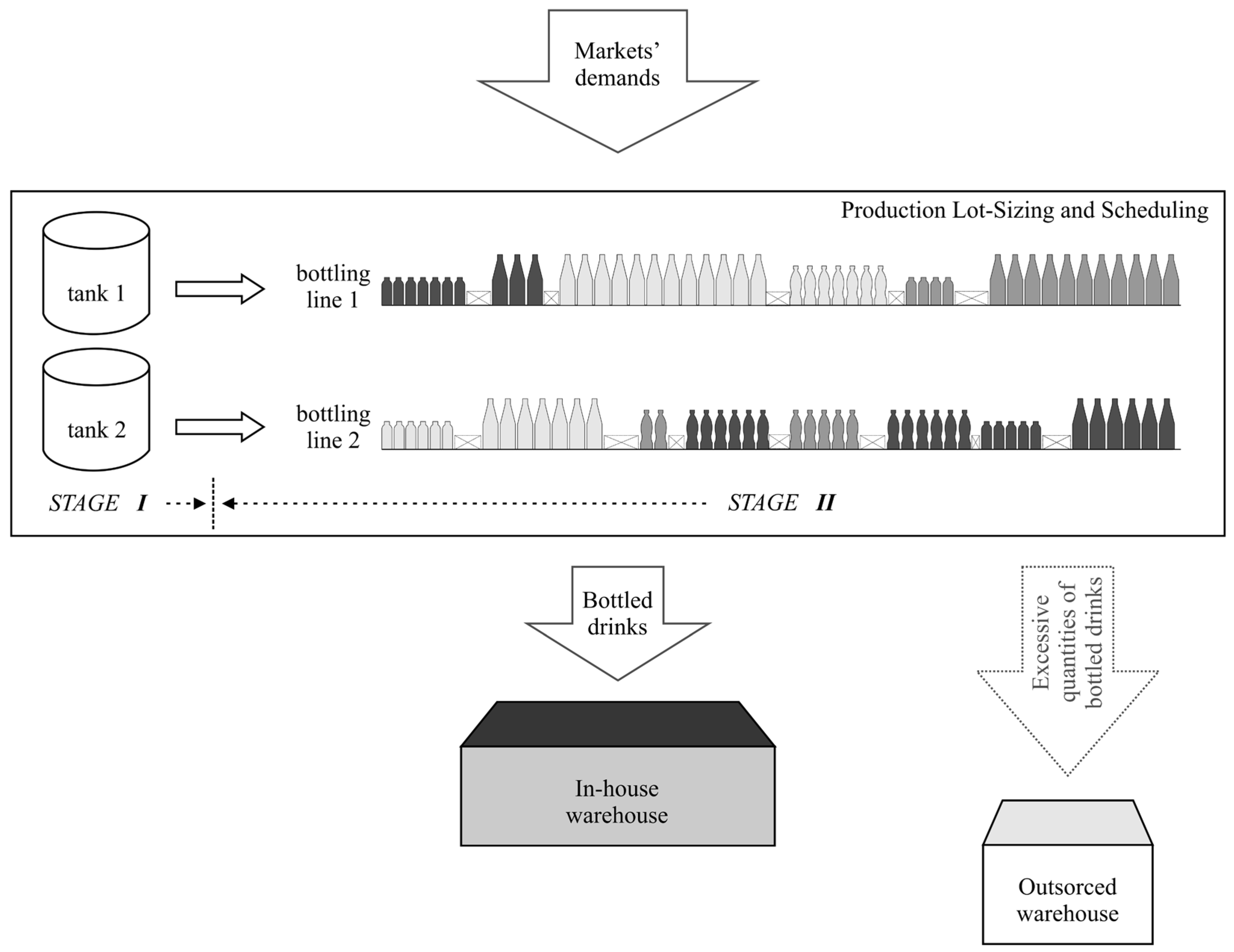
2. Problem Description
3. The Mixed Integer Linear Programming Model
- Indices:
- j - products planned for production in the planning horizon (j = 1, …, J)
- t - days in the planning horizon (t = 1, …, T)
- m - production lines (m = 1, …, M)
- l - raw material (l = 1, …, L)
- s - micro-period that corresponds to an index of production lot in day t (St is a set of micro-periods s in day t)
- Parameters:
- gj - cost of backorder cost for product j (daily per product unit)
- aj - cost of safety stock violation for product j (daily per product unit)
- bj - cost of shelf-life stock violation for product j (daily per product unit)
- c - cost of warehouse capacity overflow for all products (daily per pallet)
- w - cost of lost time from production setup (per time unit)
- u - cost of unused production time (per time unit), (idle time, not used for production or changeover)
- djt - demand of product j in day t (in product units)
- rjl - required quantity of raw material l to produce unit of product j (in L)
- aIImj - unit production time for product j in production line m
- KIm - capacity of tank m for production line m (in L)
- KIImt - available time capacity for production line m in day t
- qIlm - minimum quantity of raw material l in tank at production line m required for production (in L)
- αm - set of eligible products for production line m
- βm - set of eligible raw materials for production line m (depends on the αm).
- SSjt - minimum target safety stock level for product j in day t (in product units)
- SLjt - maximum target stock level for product j in day t (in product units)
- WHt - total warehouse capacity in pallet locations in day t (in pallets)
- WH+ - daily increase in available warehouse capacity (in pallets) due to the expected sales of products not in the production planning horizon (products in the company’s portfolio that are not in danger of stockout in the time period of T days)
- Pj - number of j product units on one pallet
- s0t - first micro-period s in day t
- STij - production setup time from the product i to j (equals to max{raw material changeover time in tanks, product changeover time on production lines}). We presume that this time has the same value for all changeovers between products, regardless of the production line.
- Decision variables:
- xIImjs - production quantity (lot size) of product j on line m in micro-period s (in product units)
- yIImjs - binary variable that takes value 1 if product j is scheduled on line m in micro-period s
- zIImijs - binary variable that takes value 1 if there is a changeover in micro-period s on line m from product i to product j.
- Wmt - total production setup time for line m in day t
- I-jt - backorder of product j in day t
- I+jt - total stock of product j in day t (in product units)
- VSSjt - violation of target minimum stock level (SSjt) for product j in day t (in product units)
- VSLjt - violation of target maximum stock level (SLjt) for product j in day t (in product units)
- VWHt - violation of warehouse capacity in day t (in pallets)
- Umt - unused production time of line m in day t
4. The Hybrid VNS/LP Model
| Algorithm 1. The outline of the proposed hybrid VNS/LP model. | |
| Termination criteria = False until the maximum allowed CPU time | |
| 1: | Construct Initial solution |
| 2: | Apply Local search procedure on Initial solution to obtain Current best solution |
| 3: | While Termination criteria == False: |
| 4: | For Sh_intensity in SoI: #Set of intensities |
| 5: | For Shaking pass in range(0, Tnp): #Total number of passes |
| 6: | Apply Shaking(Sh_intensity) move on Current best solution to obtain New solution |
| 7: | Apply Local search procedure on New solution |
| 8: | If New solution is better than Current best solution: |
| 9: | Current best solution ← New solution |
| 10: | Break to line 3 |
| Algorithm 2. The initial solution construction. | |
| Solution ← empty set of sequences and lot-sizes | |
| Improvement ← True | |
| 1: | While Improvement: |
| 2: | Best_new_solution ← Solution |
| 3: | For j in J: Define Insertion_benefit_list |
| 4: | Sort Insertion_benefit_list by highest approx. benefit |
| 5: | benefit = 0 |
| 6: | For ins in N best insertions from Insertion_benefit_list: |
| 8: | t’, j ← ins |
| 9: | For t in [t’−Δ, t’+Δ]: #evaluate Δ days before and after t’ |
| 10: | For m in M: |
| 11: | New_solution ← insertion for j,t,m i n Solution #using LP model |
| 12: | If cost(Solution) − cost(New_solution) > benefit: |
| 13: | benefit = cost(Solution) − cost(New_solution) |
| 14: | Best_new_solution ← New_solution |
| 15: | If benefit > 0: |
| 16: | Solution ← Best_new_solution |
| 17: | Else: Improvement = False |
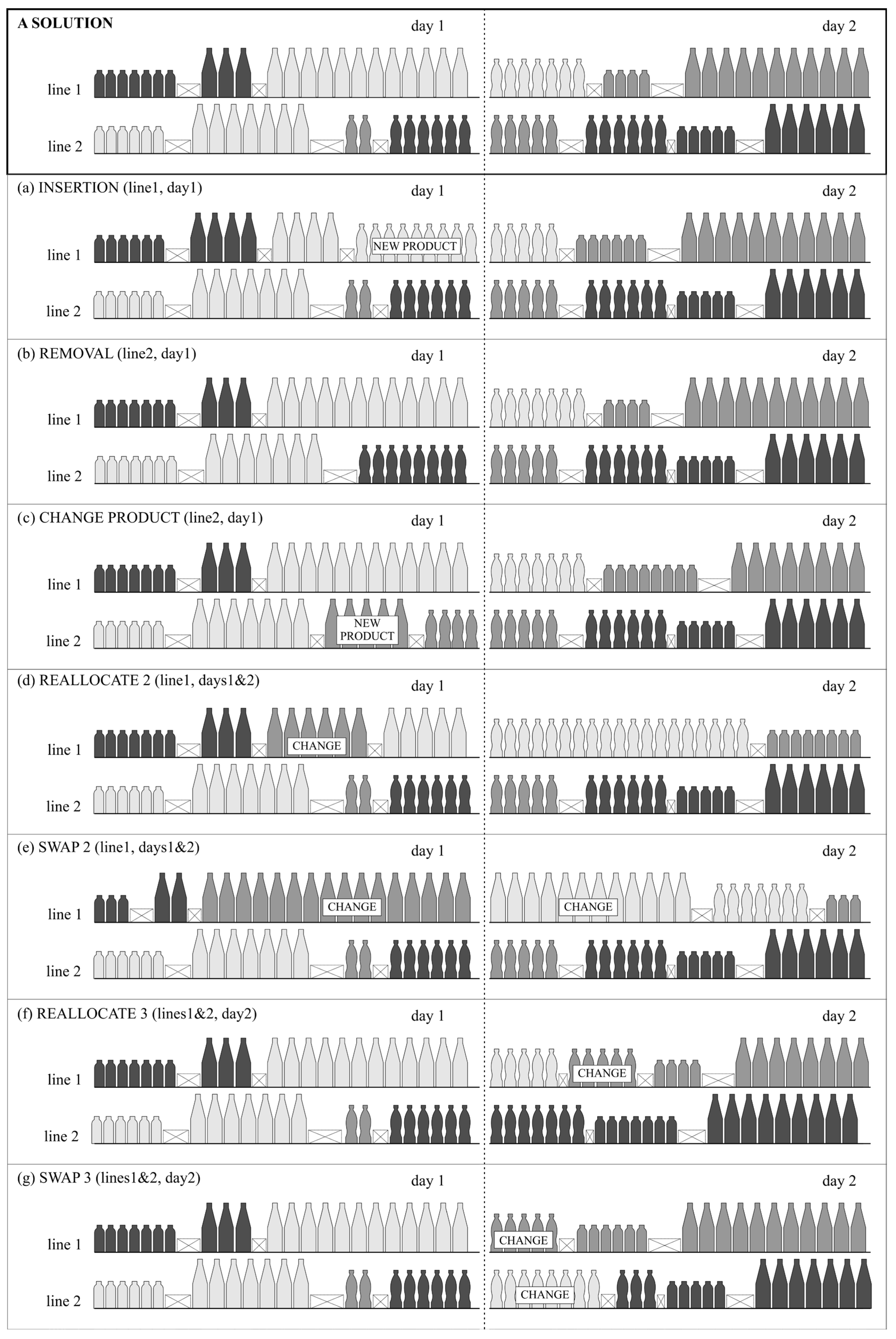
| (a) Insertion | - of a new product on line m in day t |
| (b) Removal | - of a product j on line m in day t |
| (c) Change product | - for line m in day t, removal of a product j and insertion of a new product j* |
| (d) Reallocate 2 | - reallocate product j on line m from day t1 to day t2 |
| (e) Swap 2 | - for line m, swap product j1 from day t1 with product j2 from day t2 |
| (f) Reallocate 3 | - reallocate product j in day t from line m1 to line m2 |
| (g) Swap 3 | - for day t, swap product j1 from line m1 with product j2 from line m2 |
| Algorithm 3. The local search procedure. | |
| Input Current_best_solution | |
| Randomize order of neighborhoods in List_of_neighborhoods | |
| Improvement ← True | |
| 1: | While Improvement: |
| 2: | Improvement = False |
| 3: | For neighborhood in List_of_neighborhoods: |
| 4: | For move in neighborhood: #iterate trough all possible search moves |
| 5: | Generate random_number from [0.0, 1.0] |
| 6: | If random_number < PLS: |
| 7: | New_solution ← Current_best_solution & move |
| 8: | If New_solution is better than Current_best_solution: |
| 9: | Current_best_solution ← New_solution |
| 10: | Improvement = True |
| Algorithm 4. The shaking procedure. | |
| Input Current_best_solution; Sh_intensity | |
| 1: | For change in range(1, Sh_intensity+1): |
| 2: | Apply a random Removal, Insertion, and Change Product |
| 3: | If change/Max_intensity > RS1: |
| 4: | Remove all j from one random t of one random m |
| 5: | If change/Max_intensity > RS2: |
| 6: | Apply a random Reallocate 2, and Swap 2 |
| 7: | If change/Max_intensity > RS3: |
| 8: | Apply a random Reallocate 3, and Swap 3 |
| 9: | If change/Max_intensity > RS4: |
| 10: | Apply one random change from each neighborhood used in shaking |
- nsmjt - number of production lots for product j on line m in day t
- Wmt - production setup time for line m in day t
- uIImjt - lot size for product j on line m in day t. From uIImjt, other decision variables are derived and used in objective function (18) to obtain the values of five sub-objectives.
- VPTmt - the violation of production time of line m in day t
- Ω - big number (coefficient used to eliminate solutions with a production time violation in the process of finding the best solution in the proposed hybrid approach)
5. Test Instances and Computational Results
- Small-scale instances
- - KIImt = 8 h; J = 10 products; L = 6 raw materials; T = 3 days; 3 micro-periods per day; WH0 = 1000 pallets
- Large-scale instances
- - KIImt = 20 h; J = 30 products; L = 20 raw materials; T = 10 days; 5 micro-periods per day; WH0 = 3000 pallets
- - basic variant with two production lines (both can bottle all products); input parameters for one small-scale instance are presented in Table 3
- - increased production-time-related costs by 25% (setup time and unused time costs)
- - smaller starting warehouse capacity by 25%; increase in outsourced warehousing cost by 25%
- - increased inventory-related costs by 25% (backorder, minimum safety stock and shelf-life stock violations)
- - increased product demand (including minimum and maximum stock level) by 25%
- Initial solution (BRI) - N = 2 and Δ = 1 for small-scale instances, and N = 3 and Δ = 2 for large-scale instances
- Local search - PSL = 0.5
- Shaking - SoI = [1,2,3,4,5,6,7,8,9,10]; RS1 = 0.4, RS2 = 0.5, RS3 = 0.6, RS4 = 0.7; Tnp = 1 and Tnp = 2 for small and large-scale instances, respectively
- Termination criterion - max CPU time was set to 60 s and 14,400 s for small- and large-scale instances, respectively
5.1. Small-Scale Instance Computational Results
5.2. Large-Scale Instance Computational Results
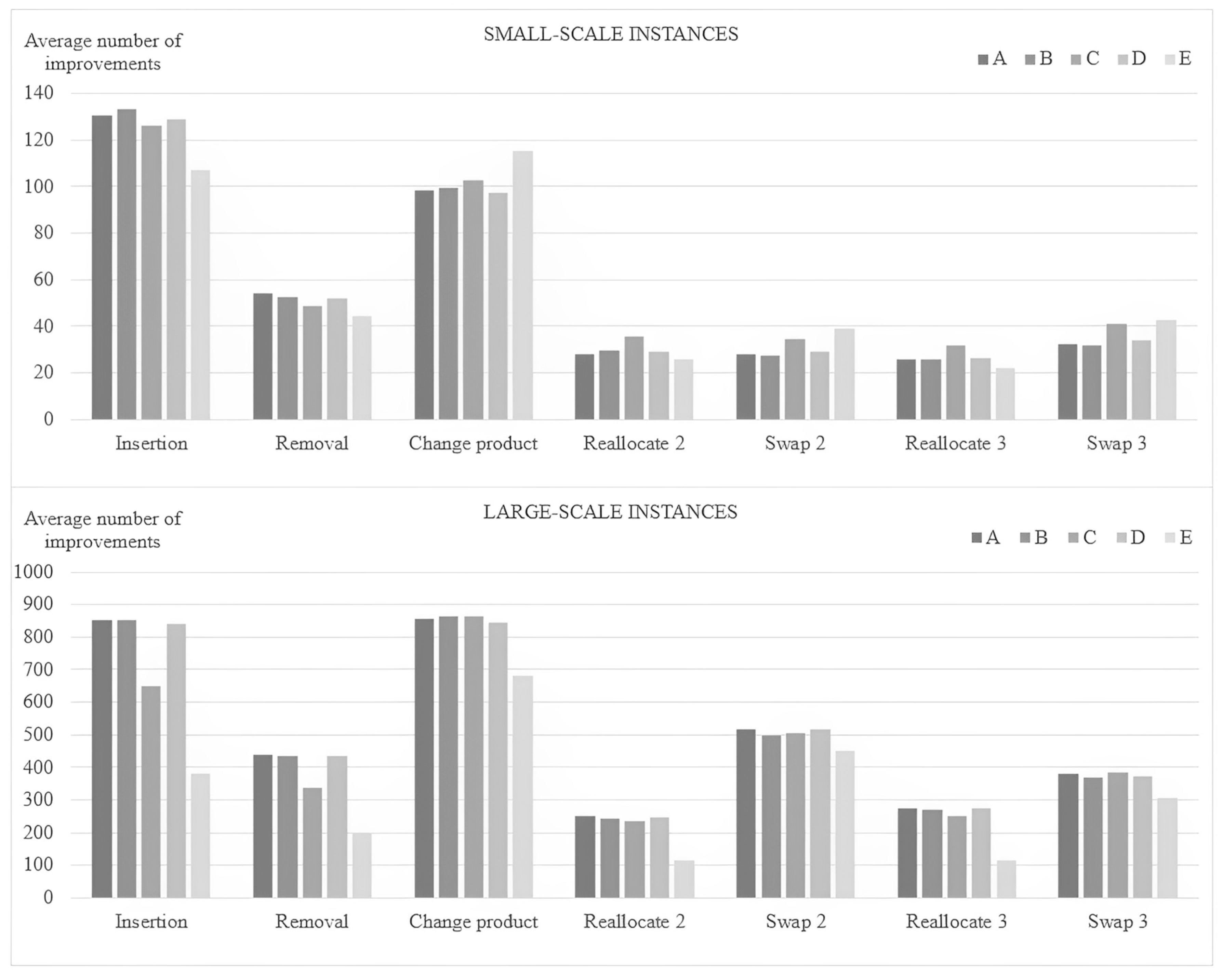
5.3. The Effectiveness of Neighborhoods Used in the Local Search Procedure
6. Concluding Remarks
Supplementary Materials
Author Contributions
Funding
Data Availability Statement
Conflicts of Interest
References
- Clark, A.; Almada-Lobo, B.; Almeder, C. Lot Sizing and Scheduling: Industrial Extensions and Research Opportunities. Int. J. Prod. Res. 2011, 49, 2457–2461. [Google Scholar] [CrossRef] [Green Version]
- Kopanos, G.M.; Puigjaner, L. Solving Large-Scale Production Scheduling and Planning in the Process Industries; Springer International Publishing: Cham, Switzerland, 2019; ISBN 978-3-030-01182-6. [Google Scholar]
- Ferreira, D.; Clark, A.R.; Almada-Lobo, B.; Morabito, R. Single-Stage Formulations for Synchronised Two-Stage Lot Sizing and Scheduling in Soft Drink Production. Int. J. Prod. Econ. 2012, 136, 255–265. [Google Scholar] [CrossRef]
- Ferreira, D.; Morabito, R.; Rangel, S. Solution Approaches for the Soft Drink Integrated Production Lot Sizing and Scheduling Problem. Eur. J. Oper. Res. 2009, 196, 697–706. [Google Scholar] [CrossRef]
- Ferreira, D.; Morabito, R.; Rangel, S. Relax and Fix Heuristics to Solve One-Stage One-Machine Lot-Scheduling Models for Small-Scale Soft Drink Plants. Comput. Oper. Res. 2010, 37, 684–691. [Google Scholar] [CrossRef]
- Pagliarussi, M.S.; Morabito, R.; Santos, M.O. Otimização Da Programação Da Produção de Bebidas à Base de Frutas Por Meio de Modelos de Programação Inteira Mista. Gest. Produção 2016, 24, 64–77. [Google Scholar] [CrossRef] [Green Version]
- Toledo, C.F.M.; de Oliveira, L.; de Freitas Pereira, R.; França, P.M.; Morabito, R. A Genetic Algorithm/Mathematical Programming Approach to Solve a Two-Level Soft Drink Production Problem. Comput. Oper. Res. 2014, 48, 40–52. [Google Scholar] [CrossRef]
- Toledo, C.F.M.; França, P.M.; Morabito, R.; Kimms, A. Multi-Population Genetic Algorithm to Solve the Synchronized and Integrated Two-Level Lot Sizing and Scheduling Problem. Int. J. Prod. Res. 2009, 47, 3097–3119. [Google Scholar] [CrossRef] [Green Version]
- Toscano, A.; Ferreira, D.; Morabito, R. A Decomposition Heuristic to Solve the Two-Stage Lot Sizing and Scheduling Problem with Temporal Cleaning. Flex. Serv. Manuf. J. 2019, 31, 142–173. [Google Scholar] [CrossRef]
- Baldo, T.A.; Santos, M.O.; Almada-Lobo, B.; Morabito, R. An Optimization Approach for the Lot Sizing and Scheduling Problem in the Brewery Industry. Comput. Ind. Eng. 2014, 72, 58–71. [Google Scholar] [CrossRef]
- Claassen, G.D.H.; Gerdessen, J.C.; Hendrix, E.M.T.; van der Vorst, J.G.A.J. On Production Planning and Scheduling in Food Processing Industry: Modelling Non-Triangular Setups Andproduct Decay. Comput. Oper. Res. 2016, 76, 147–154. [Google Scholar] [CrossRef]
- Shin, M.; Lee, H.; Ryu, K.; Cho, Y.; Son, Y.-J. A Two-Phased Perishable Inventory Model for Production Planning in a Food Industry. Comput. Ind. Eng. 2019, 133, 175–185. [Google Scholar] [CrossRef]
- Soler, W.A.O.; Santos, M.O.; Akartunalı, K. MIP Approaches for a Lot Sizing and Scheduling Problem on Multiple Production Lines with Scarce Resources, Temporary Workstations, and Perishable Products. J. Oper. Res. Soc. 2019, 72, 1691–1706. [Google Scholar] [CrossRef]
- Entrup, M.L.; Günther, H.-O.; Van Beek, P.; Grunow, M.; Seiler, T. Mixed-Integer Linear Programming Approaches to Shelf-Life-Integrated Planning and Scheduling in Yoghurt Production. Int. J. Prod. Res. 2005, 43, 5071–5100. [Google Scholar] [CrossRef]
- Marinelli, F.; Nenni, M.E.; Sforza, A. Capacitated Lot Sizing and Scheduling with Parallel Machines and Shared Buffers: A Case Study in a Packaging Company. Ann. Oper. Res. 2007, 150, 177–192. [Google Scholar] [CrossRef]
- Clark, A.R.; Morabito, R.; Toso, E.A.V. Production Setup-Sequencing and Lot-Sizing at an Animal Nutrition Plant through Atsp Subtour Elimination and Patching. J. Sched. 2010, 13, 111–121. [Google Scholar] [CrossRef]
- de Araujo, S.A.; Arenales, M.N.; Clark, A.R. Joint Rolling-Horizon Scheduling of Materials Processing and Lot-Sizing with Sequence-Dependent Setups. J. Heuristics 2007, 13, 337–358. [Google Scholar] [CrossRef]
- Wu, J.; Zhang, D.; Yang, Y.; Wang, G.; Su, L. Multi-Stage Multi-Product Production and Inventory Planning for Cold Rolling under Random Yield. Mathematics 2022, 10, 597. [Google Scholar] [CrossRef]
- Hans, E.; van de Velde, S. The Lot Sizing and Scheduling of Sand Casting Operations. Int. J. Prod. Res. 2011, 49, 2481–2499. [Google Scholar] [CrossRef]
- Silva, C.; Magalhaes, J.M. Heuristic Lot Size Scheduling on Unrelated Parallel Machines with Applications in the Textile Industry. Comput. Ind. Eng. 2006, 50, 76–89. [Google Scholar] [CrossRef] [Green Version]
- Cardona-Valdés, Y.; Nucamendi-Guillén, S.; Peimbert-García, R.E.; Macedo-Barragán, G.; Díaz-Medina, E. A New Formulation for the Capacitated Lot Sizing Problem with Batch Ordering Allowing Shortages. Mathematics 2020, 8, 878. [Google Scholar] [CrossRef]
- Almada-Lobo, B.; Oliveira, J.F.; Carravilla, M.A. Production Planning and Scheduling in the Glass Container Industry: A VNS Approach. Int. J. Prod. Econ. 2008, 114, 363–375. [Google Scholar] [CrossRef]
- Klement, N.; Abdeljaouad, M.A.; Porto, L.; Silva, C. Lot-Sizing and Scheduling for the Plastic Injection Molding Industry—A Hybrid Optimization Approach. Appl. Sci. 2021, 11, 1202. [Google Scholar] [CrossRef]
- Luche, J.R.D.; Morabito, R.; Pureza, V. Combining Process Selection and Lot Sizing Models for Production Scheduling of Electrofused Grains. Asia-Pac. J. Oper. Res. 2009, 26, 421–443. [Google Scholar] [CrossRef]
- Santos, M.O.; Almada-Lobo, B. Integrated Pulp and Paper Mill Planning and Scheduling. Comput. Ind. Eng. 2012, 63, 1–12. [Google Scholar] [CrossRef]
- Figueira, G.; Santos, M.O.; Almada-Lobo, B. A Hybrid VNS Approach for the Short-Term Production Planning and Scheduling: A Case Study in the Pulp and Paper Industry. Comput. Oper. Res. 2013, 40, 1804–1818. [Google Scholar] [CrossRef]
- Martínez, K.P.; Morabito, R.; Toso, E.A.V. A Coupled Process Configuration, Lot-Sizing and Scheduling Model for Production Planning in the Molded Pulp Industry. Int. J. Prod. Econ. 2018, 204, 227–243. [Google Scholar] [CrossRef]
- Pierini, L.M.; Poldi, K.C. Optimization of the Cutting Process Integrated to the Lot Sizing in Multi-Plant Paper Production Industries. Comput. Oper. Res. 2023, 153, 106157. [Google Scholar] [CrossRef]
- Stadtler, H. Multi-Level Single Machine Lot-Sizing and Scheduling with Zero Lead Times. Eur. J. Oper. Res. 2011, 209, 241–252. [Google Scholar] [CrossRef]
- Li, Y.; Saldanha-da-Gama, F.; Liu, M.; Yang, Z. A Risk-Averse Two-Stage Stochastic Programming Model for a Joint Multi-Item Capacitated Line Balancing and Lot-Sizing Problem. Eur. J. Oper. Res. 2023, 304, 353–365. [Google Scholar] [CrossRef]
- Wang, S.; Hui, J.; Zhu, B.; Liu, Y. Adaptive Genetic Algorithm Based on Fuzzy Reasoning for the Multilevel Capacitated Lot-Sizing Problem with Energy Consumption in Synchronizer Production. Sustainability 2022, 14, 5072. [Google Scholar] [CrossRef]
- Jans, R.; Degraeve, Z. An Industrial Extension of the Discrete Lot-Sizing and Scheduling Problem. IIE Trans. 2004, 36, 47–58. [Google Scholar] [CrossRef]
- Xiao, J.; Yang, H.; Zhang, C.; Zheng, L.; Gupta, J.N.D. A Hybrid Lagrangian-Simulated Annealing-Based Heuristic for the Parallel-Machine Capacitated Lot-Sizing and Scheduling Problem with Sequence-Dependent Setup Times. Comput. Oper. Res. 2015, 63, 72–82. [Google Scholar] [CrossRef]
- Pressmar, D.B. Modellierung und Optimierung dynamischer Produktionssysteme. In Modellierung und Optimierung Dynamischer Produktionssysteme; De Gruyter: Berlin, Germany, 1980; pp. 453–470. ISBN 978-3-11-086695-7. [Google Scholar]
- Fleischmann, B.; Meyr, H. The General Lotsizing and Scheduling Problem. Oper.-Res.-Spektrum 1997, 19, 11–21. [Google Scholar] [CrossRef]
- Fleischmann, B. The Discrete Lot-Sizing and Scheduling Problem with Sequence-Dependent Setup Costs. Eur. J. Oper. Res. 1994, 75, 395–404. [Google Scholar] [CrossRef]
- Haase, K. Capacitated Lot-Sizing with Sequence Dependent Setup Costs. Oper.-Res.-Spektrum 1996, 18, 51–59. [Google Scholar] [CrossRef] [Green Version]
- Meyr, H. Simultaneous Lotsizing and Scheduling on Parallel Machines. Eur. J. Oper. Res. 2002, 139, 277–292. [Google Scholar] [CrossRef]
- Copil, K.; Wörbelauer, M.; Meyr, H.; Tempelmeier, H. Simultaneous Lotsizing and Scheduling Problems: A Classification and Review of Models. Spectrum 2017, 39, 1–64. [Google Scholar] [CrossRef]
- Drexl, A.; Kimms, A. Lot Sizing and Scheduling—Survey and Extensions. Eur. J. Oper. Res. 1997, 99, 221–235. [Google Scholar] [CrossRef] [Green Version]
- Kuik, R.; Salomon, M.; Van Wassenhove, L.N.; Maes, J. Linear Programming, Simulated Annealing and Tabu Search Heuristics for Lotsizing in Bottleneck Assembly Systems. IIE Trans. 1993, 25, 62–72. [Google Scholar] [CrossRef]
- Meyr, H. Simultaneous Lotsizing and Scheduling by Combining Local Search with Dual Reoptimization. Eur. J. Oper. Res. 2000, 120, 311–326. [Google Scholar] [CrossRef]
- Almada-Lobo, B.; James, R.J.W. Neighbourhood Search Meta-Heuristics for Capacitated Lot-Sizing with Sequence-Dependent Setups. Int. J. Prod. Res. 2010, 48, 861–878. [Google Scholar] [CrossRef]
- Xiao, Y.; Zhang, R.; Zhao, Q.; Kaku, I.; Xu, Y. A Variable Neighborhood Search with an Effective Local Search for Uncapacitated Multilevel Lot-Sizing Problems. Eur. J. Oper. Res. 2014, 235, 102–114. [Google Scholar] [CrossRef] [Green Version]
- Xiao, Y.; Kaku, I.; Zhao, Q.; Zhang, R. A Variable Neighborhood Search Based Approach for Uncapacitated Multilevel Lot-Sizing Problems. Comput. Ind. Eng. 2011, 60, 218–227. [Google Scholar] [CrossRef]
- Xiao, Y.; Kaku, I.; Zhao, Q.; Zhang, R. A Reduced Variable Neighborhood Search Algorithm for Uncapacitated Multilevel Lot-Sizing Problems. Eur. J. Oper. Res. 2011, 214, 223–231. [Google Scholar] [CrossRef]
- Silver, E.A. Shelf Life Considerations in a Family Production Context. Int. J. Prod. Res. 1989, 27, 2021–2026. [Google Scholar] [CrossRef]
- Mladenović, N.; Hansen, P. Variable Neighborhood Search. Comput. Oper. Res. 1997, 24, 1097–1100. [Google Scholar] [CrossRef]
- Mladenović, N. A Variable Neighborhood Algorithm—A New Metaheuristic for Combinatorial Optimization. In Book of Abstracts, Optimization Days; Montreal, QC, Canada, 1995. [Google Scholar]
- Hansen, P.; Mladenović, N. Variable Neighborhood Search. In Handbook of Heuristics; Martí, R., Pardalos, P.M., Resende, M.G.C., Eds.; Springer International Publishing: Cham, Switzerland, 2018; pp. 759–787. ISBN 978-3-319-07124-4. [Google Scholar]
- Hansen, P.; Mladenović, N.; Todosijević, R.; Hanafi, S. Variable Neighborhood Search: Basics and Variants. EURO J. Comput. Optim. 2017, 5, 423–454. [Google Scholar] [CrossRef]


| References | Application Area |
|---|---|
| Ferreira et al. [3,4,5], Pagliarussi et al. [6], Toledo et al. [7,8], Toscano et al. [9] | Soft drink industry |
| Baldo et al. [10] | Brewery industry |
| Claassen et al. [11], Shin et al. [12], Soler et al. [13], Lütke et al. [14], Marinelli et al. [15], Clark et al. [16] | Food processing industry |
| Araujo et al. [17], Wu et al. [18], Hans and Van de Velde [19] | Metal industry |
| Silva and Magalhaes [20], Cardona-Valdés et al. [21] | Textile industry |
| Almada-Lobo et al. [22] | Glass container industry |
| Klement et al. [23] | Molded plastic industry |
| Luche et al. [24] | Grain industry |
| Santos and Almada-Lobo [25] and Figueira at al. [26] and Martínez [27], Livia et al. [28] | Paper manufacturing industry |
| Stadtler [29] | Pharmaceutical industry |
| Li at al. [30] | Mask production industry |
| Wang et al. [31], Jans and Deagraeve [32] | Automobile industry |
| Xiao et al. [33] | Chipset production industry |
| Reference | Solution Approach | Specific Objective Function Segments | ||||||
|---|---|---|---|---|---|---|---|---|
| Inventory | Backorder | Prod. Setup Time | Unused Prod. Time | Min. and Max. Stock Level Violation | Warehouse Capacity Overflow | Problem Scale | ||
| Ferreira et al. [5] | MIP, relax and fix heuristics | ✓ | ✓ | ✓ | Reduced to stage II | |||
| Ferreira et al. [3] | MIP, Asymmetric Travelling Salesman Problem | ✓ | ✓ | ✓ | Stage I and II | |||
| Baldo et al. [10] | MIP, MIP-based heuristic | ✓ | ✓ | ✓ | Stage I and II | |||
| Pagliarussi et al. [6] | MIP | ✓ | ✓ | ✓ | Reduced to stage II | |||
| Toledo et al. [8] | MIP branch and cut, GA | ✓ | ✓ | ✓ | Stage I and II | |||
| Toledo et al. [7] | MIP, GA/mathematical programming approach | ✓ | ✓ | ✓ | Stage I and II | |||
| Toscano et al. [9] | MIP/two-phase heuristic | ✓ | ✓ | ✓ | Stage I and II | |||
| This paper | MILP, VNS/LP heuristic | ✓ * | ✓ | ✓ | ✓ | ✓ | ✓ | Stage I and II |
| Input Data | Values |
|---|---|
| WHt | = [1000, 1170, 1340] |
| Pj | = [1584, 1584, 1584, 1296, 1296, 1296, 1296, 504, 504, 504] |
| gj | = [0.28, 0.3, 0.36, 0.14, 0.34, 0.24, 0.12, 0.2, 0.1, 0.34] |
| aj | = [0.14, 0.15, 0.18, 0.07, 0.17, 0.12, 0.06, 0.1, 0.05, 0.17] |
| bj | = [0.056, 0.06, 0.072, 0.028, 0.068, 0.048, 0.024, 0.04, 0.02, 0.068] |
| djt (for all t) | = [19,019, 18,880, 14,933, 19,405, 12,030, 4559, 19,633, 23,867, 18,545, 5237] |
| SSjt (for all t) | = [95,095, 94,400, 74,665, 97,025, 60,150, 22,795, 98,165, 119,335, 92,725, 26,185] |
| SLjt (for all t) | = [1,141,140, 1,132,800, 895,980, 1,164,300, 721,800, 273,540, 1,177,980, 1,432,020, 1,112,700, 314,220] |
| I+j0 | = [149,679, 147,075, 105,277, 120,505, 74,826, 35,469, 78,532, 90,813, 130,742, 34,668] |
| rjl [l = 1] | = [0.33, -, -, -, -, -, -, -, 1.5, - ] |
| rjl [l = 2] | = [-, -, -, -, -, 0.5, -, -, -, - ] |
| rjl [l = 3] | = [-, 0.33, -, 0.5, -, -, -, -, -, - ] |
| rjl [l = 4] | = [-, -, -, -, -, -, 0.5, -, -, - ] |
| rjl [l = 5] | = [-, -, -, -, -, -, -, -, -, 1.5 ] |
| rjl [l = 6] | = [-, -, 0.33, -, 0.5, -, -, 1.5, -, - ] |
| STij [i = 1] | = [30, 240, 120, 240, 120, 240, 240, 240, 60, 120 ] |
| STij [i = 2] | = [120, 30, 120, 240, 240, 60, 120, 240, 240, 120 ] |
| STij [i = 3] | = [120, 120, 30, 120, 120, 120, 60, 120, 120, 120 ] |
| STij [i = 4] | = [120, 240, 240, 30, 120, 60, 120, 120, 120, 60 ] |
| STij [i = 5] | = [120, 120, 120, 120, 30, 120, 60, 120, 240, 120 ] |
| STij [i = 6] | = [240, 120, 120, 60, 120, 30, 30, 240, 120, 120 ] |
| STij [i = 7] | = [120, 240, 240, 60, 120, 30, 30, 120, 240, 240 ] |
| STij [i = 8] | = [120, 120, 120, 120, 60, 240, 120, 30, 120, 120 ] |
| STij [i = 9] | = [240, 240, 120, 240, 120, 240, 240, 120, 30, 120 ] |
| STij [i = 10] | = [120, 60, 240, 120, 120, 240, 120, 60, 120, 30 ] |
| aIImj [m = 1] | = [0.0036, 0.0036, 0.0036, 0.0036, 0.0036, 0.0036, 0.0036, 0.005, 0.005, 0.005] |
| aIImj [m = 2] | = [0.0036, 0.0036, 0.0036, 0.0036, 0.0036, 0.0036, 0.0036, 0.005, 0.005, 0.005] |
| The MILp Model | The Hybrid VNS/LP Model | Difference | CV [%] | |||||||||||
|---|---|---|---|---|---|---|---|---|---|---|---|---|---|---|
| Total Costs [€] | [%] | |||||||||||||
| Inst. | Total Costs [€] | VSS Cost [€] | VWH Cost [€] | W Cost [€] | U Cost [€] | CPU Time [s] | Avg | Stdev | Min | Max | Avg | Min | ||
| A | 1 | 1369.83 | 120.36 | 289.47 | 960 | 0.00 | 1408 | 1408.16 | 91.33 | 1369.83 | 1633.10 | 2.80 | 0.00 | 6.49 |
| 2 | 667.49 | 67.49 | 0.00 | 600 | 0.00 | 1567 | 667.49 | 0.00 | 667.49 | 667.49 | 0.00 | 0.00 | 0.00 | |
| 3 | 528.78 | 0.00 | 48.78 | 480 | 0.00 | 908 | 532.83 | 9.64 | 528.78 | 555.78 | 0.77 | 0.00 | 1.81 | |
| 4 | 1048.51 | 325.93 | 122.58 | 600 | 0.00 | 359 | 1050.23 | 5.14 | 1048.51 | 1065.65 | 0.16 | 0.00 | 0.49 | |
| 5 | 969.63 | 85.70 | 306.05 | 480 | 97.88 | 239 | 969.63 | 0.00 | 969.63 | 969.63 | 0.00 | 0.00 | 0.00 | |
| 6 | 1528.63 | 292.90 | 515.73 | 720 | 0.00 | 485 | 1599.36 | 88.55 | 1528.63 | 1728.34 | 4.63 | 0.00 | 5.54 | |
| 7 | 960.00 | 0.00 | 0.00 | 960 | 0.00 | 2095 | 960.00 | 0.00 | 960.00 | 960.00 | 0.00 | 0.00 | 0.00 | |
| 8 | 840.00 | 0.00 | 0.00 | 840 | 0.00 | 914 | 840.00 | 0.00 | 840.00 | 840.00 | 0.00 | 0.00 | 0.00 | |
| 9 | 1481.00 | 161.00 | 0.00 | 1320 | 0.00 | 393 | 1498.61 | 42.20 | 1481.00 | 1659.06 | 1.19 | 0.00 | 2.82 | |
| 10 | 1181.35 | 0.00 | 461.35 | 720 | 0.00 | 1199 | 1203.18 | 29.87 | 1181.35 | 1291.65 | 1.85 | 0.00 | 2.48 | |
| Avg | 1057.52 | 105.34 | 174.40 | 768 | 9.79 | 957 | 1072.95 | 1.14 | 0.00 | 1.96 | ||||
| B | 1 | 1609.83 | 120.36 | 289.47 | 1200 | 0.00 | 558 | 1624.26 | 43.27 | 1609.83 | 1754.05 | 0.90 | 0.00 | 2.66 |
| 2 | 817.49 | 67.49 | 0.00 | 750 | 0.00 | 1384 | 817.49 | 0.00 | 817.49 | 817.49 | 0.00 | 0.00 | 0.00 | |
| 3 | 645.78 | 195.78 | 0.00 | 450 | 0.00 | 1228 | 645.78 | 0.00 | 645.78 | 645.78 | 0.00 | 0.00 | 0.00 | |
| 4 | 1155.65 | 583.07 | 122.58 | 450 | 0.00 | 96 | 1157.80 | 9.34 | 1155.65 | 1198.51 | 0.19 | 0.00 | 0.81 | |
| 5 | 1114.10 | 85.70 | 306.05 | 600 | 122.35 | 181 | 1117.85 | 11.25 | 1114.10 | 1151.60 | 0.34 | 0.00 | 1.01 | |
| 6 | 1708.63 | 292.90 | 515.73 | 900 | 0.00 | 141 | 1734.12 | 45.73 | 1708.63 | 1846.41 | 1.49 | 0.00 | 2.64 | |
| 7 | 1182.38 | 282.38 | 0.00 | 900 | 0.00 | 1559 | 1182.38 | 0.00 | 1182.38 | 1182.38 | 0.00 | 0.00 | 0.00 | |
| 8 | 1050.00 | 0.00 | 0.00 | 1050 | 0.00 | 1550 | 1050.00 | 0.00 | 1050.00 | 1050.00 | 0.00 | 0.00 | 0.00 | |
| 9 | 1809.06 | 459.06 | 0.00 | 1350 | 0.00 | 343 | 1809.25 | 0.58 | 1809.06 | 1811.00 | 0.01 | 0.00 | 0.03 | |
| 10 | 1361.35 | 0.00 | 461.35 | 900 | 0.00 | 753 | 1371.09 | 20.77 | 1361.35 | 1455.33 | 0.72 | 0.00 | 1.51 | |
| Avg | 1245.43 | 208.67 | 169.52 | 855 | 12.24 | 779 | 1251.00 | 0.37 | 0.00 | 0.87 | ||||
| C | 1 | 4379.81 | 120.36 | 2966.43 | 960 | 333.02 | 441 | 4383.53 | 11.72 | 4379.81 | 4428.39 | 0.08 | 0.00 | 0.27 |
| 2 | 1936.90 | 67.49 | 447.89 | 960 | 461.52 | 488 | 1954.75 | 22.24 | 1936.90 | 2012.46 | 0.92 | 0.00 | 1.14 | |
| 3 | 2828.32 | 195.78 | 823.99 | 480 | 1328.55 | 29 | 2846.33 | 25.23 | 2828.32 | 2910.82 | 0.64 | 0.00 | 0.89 | |
| 4 | 3280.86 | 183.04 | 2017.82 | 1080 | 0.00 | 803 | 3462.76 | 92.09 | 3280.86 | 3526.79 | 5.54 | 0.00 | 2.66 | |
| 5 | 3931.60 | 85.70 | 2358.46 | 840 | 647.43 | 247 | 3938.30 | 13.49 | 3931.60 | 3968.58 | 0.17 | 0.00 | 0.34 | |
| 6 | 4238.69 | 165.54 | 2633.15 | 1440 | 0.00 | 1496 | 4253.76 | 19.35 | 4238.69 | 4324.26 | 0.36 | 0.00 | 0.45 | |
| 7 | 1771.65 | 0.00 | 305.22 | 960 | 506.42 | 249 | 1804.67 | 32.83 | 1771.65 | 1868.40 | 1.86 | 0.00 | 1.82 | |
| 8 | 2315.39 | 0.00 | 765.71 | 960 | 589.68 | 75 | 2356.88 | 24.97 | 2315.39 | 2400.54 | 1.79 | 0.00 | 1.06 | |
| 9 | 3716.21 | 179.43 | 1976.78 | 1560 | 0.00 | 1145 | 3741.05 | 47.20 | 3716.21 | 3851.89 | 0.67 | 0.00 | 1.26 | |
| 10 | 4031.51 | 339.48 | 2871.01 | 600 | 221.03 | * 3600 | 4042.13 | 14.61 | 4031.51 | 4070.74 | 0.26 | 0.00 | 0.36 | |
| Avg | 3243.09 | 133.68 | 1716.65 | 984 | 408.77 | 857 | 3278.42 | 1.23 | 0.00 | 1.03 | ||||
| D | 1 | 1399.92 | 150.45 | 289.47 | 960 | 0.00 | 811 | 1399.92 | 0.00 | 1399.92 | 1399.92 | 0.00 | 0.00 | 0.00 |
| 2 | 684.36 | 84.36 | 0.00 | 600 | 0.00 | 1445 | 684.36 | 0.00 | 684.36 | 684.36 | 0.00 | 0.00 | 0.00 | |
| 3 | 528.78 | 0.00 | 48.78 | 480 | 0.00 | 881 | 539.46 | 25.43 | 528.78 | 600.00 | 2.02 | 0.00 | 4.71 | |
| 4 | 1130.00 | 407.41 | 122.58 | 600 | 0.00 | 195 | 1138.14 | 24.43 | 1130.00 | 1211.42 | 0.72 | 0.00 | 2.15 | |
| 5 | 991.05 | 107.13 | 306.05 | 480 | 97.88 | 295 | 1005.41 | 47.49 | 991.05 | 1197.91 | 1.45 | 0.00 | 4.72 | |
| 6 | 1601.85 | 366.13 | 515.73 | 720 | 0.00 | 321 | 1669.91 | 101.30 | 1601.85 | 1923.60 | 4.25 | 0.00 | 6.07 | |
| 7 | 960.00 | 0.00 | 0.00 | 960 | 0.00 | 1631 | 960.00 | 0.00 | 960.00 | 960.00 | 0.00 | 0.00 | 0.00 | |
| 8 | 840.00 | 0.00 | 0.00 | 840 | 0.00 | 1061 | 840.00 | 0.00 | 840.00 | 840.00 | 0.00 | 0.00 | 0.00 | |
| 9 | 1521.25 | 201.25 | 0.00 | 1320 | 0.00 | 364 | 1547.77 | 53.03 | 1521.25 | 1653.83 | 1.74 | 0.00 | 3.43 | |
| 10 | 1181.35 | 0.00 | 461.35 | 720 | 0.00 | 999 | 1212.67 | 47.83 | 1181.35 | 1285.73 | 2.65 | 0.00 | 3.94 | |
| Avg | 1083.86 | 131.67 | 174.40 | 768 | 9.79 | 800 | 1099.76 | 1.28 | 0.00 | 2.50 | ||||
| E | 1 | 17,025.49 | 15,006.24 | 339.24 | 1680 | 0.00 | * 3600 | 17,436.19 | 422.54 | 17,025.49 | 18,133.88 | 2.41 | 0.00 | 2.42 |
| 2 | 2752.42 | 952.42 | 0.00 | 1800 | 0.00 | 140 | 2943.54 | 235.49 | 2752.42 | 3298.03 | 6.94 | 0.00 | 8.00 | |
| 3 | 1210.25 | 130.25 | 0.00 | 1080 | 0.00 | 70 | 1260.68 | 52.68 | 1210.25 | 1450.25 | 4.17 | 0.00 | 4.18 | |
| 4 | 16,508.71 | 15,188.71 | 0.00 | 1320 | 0.00 | 972 | 16,623.57 | 216.28 | 16,508.71 | 17,264.36 | 0.70 | 0.00 | 1.30 | |
| 5 | 14,725.33 | 13,661.05 | 104.28 | 960 | 0.00 | * 3600 | 14,999.34 | 262.63 | 14,725.33 | 15,358.59 | 1.86 | 0.00 | 1.75 | |
| 6 | 24,296.25 | 22,769.38 | 206.88 | 1320 | 0.00 | * 3600 | 25,053.78 | 268.60 | 24,484.38 | 25,449.34 | 3.12 | 0.77 | 1.07 | |
| 7 | 3176.07 | 1736.07 | 0.00 | 1440 | 0.00 | 184 | 3205.17 | 89.92 | 3176.07 | 3535.16 | 0.92 | 0.00 | 2.81 | |
| 8 | 4057.90 | 2137.90 | 0.00 | 1920 | 0.00 | 257 | 4442.31 | 378.22 | 4057.90 | 5421.86 | 9.47 | 0.00 | 8.51 | |
| 9 | 30,405.42 | 29,085.42 | 0.00 | 1320 | 0.00 | 1689 | 30,473.46 | 255.90 | 30,405.42 | 31,573.86 | 0.22 | 0.00 | 0.84 | |
| 10 | 17,134.78 | 15,381.21 | 73.58 | 1680 | 0.00 | * 3600 | 17,578.61 | 393.72 | 17,134.78 | 18,405.39 | 2.59 | 0.00 | 2.24 | |
| Avg | 13,129.26 | 11,604.86 | 72.40 | 1452 | 0.00 | 1771 | 13,401.67 | 3.24 | 0.08 | 3.31 | ||||
| Total Avg | 3951.83 | 2436.85 | 461.47 | 965.40 | 88.12 | 1033 | 4220.76 | 1.45 | 0.02 | 1.93 | ||||
| Total Costs [€] | Partial Costs [€] | Diff. of Avg to Min [%] | CV [%] | |||||||||
|---|---|---|---|---|---|---|---|---|---|---|---|---|
| Inst. | Avg | Stdev | Min | Max | I- Cost | VSS Cost | VWH Cost | W Cost | U Cost | |||
| A | 1 | 8569.46 | 257.72 | 8222.75 | 9058.43 | 0.00 | 286.57 | 416.89 | 7836.00 | 30.00 | 4.22 | 3.01 |
| 2 | 5562.91 | 167.29 | 5308.48 | 5872.97 | 0.00 | 2.85 | 180.06 | 5340.00 | 40.00 | 4.79 | 3.01 | |
| 3 | 3723.06 | 222.43 | 3295.54 | 4051.39 | 0.00 | 75.72 | 141.35 | 3336.00 | 170.00 | 12.97 | 5.97 | |
| 4 | 11,584.90 | 353.00 | 11,017.14 | 12,142.37 | 0.00 | 1710.94 | 333.96 | 9540.00 | 0.00 | 5.15 | 3.05 | |
| 5 | 7337.13 | 175.28 | 7008.97 | 7548.19 | 0.00 | 121.36 | 449.77 | 6756.00 | 10.00 | 4.68 | 2.39 | |
| 6 | 5750.46 | 207.06 | 5290.54 | 6133.85 | 0.00 | 104.95 | 109.51 | 5496.00 | 40.00 | 8.69 | 3.60 | |
| 7 | 17,026.30 | 726.85 | 15,507.13 | 17,884.30 | 0.00 | 4160.51 | 25.25 | 12,828.00 | 12.55 | 9.80 | 4.27 | |
| 8 | 12,899.19 | 603.95 | 12,141.20 | 14,280.53 | 0.00 | 2537.55 | 533.65 | 9768.00 | 60.00 | 6.24 | 4.68 | |
| 9 | 4891.94 | 119.27 | 4724.31 | 5056.31 | 0.00 | 79.20 | 404.75 | 4308.00 | 100.00 | 3.55 | 2.44 | |
| 10 | 5517.82 | 141.32 | 5257.68 | 5793.42 | 0.00 | 91.87 | 413.95 | 4992.00 | 20.00 | 4.95 | 2.56 | |
| Avg | 8286.32 | 0.00 | 917.15 | 300.91 | 7020.00 | 48.25 | 6.50 | 3.50 | ||||
| B | 1 | 10,445.15 | 303.24 | 10,166.58 | 11,022.20 | 0.00 | 355.31 | 444.84 | 9570.00 | 75.00 | 2.74 | 2.90 |
| 2 | 7020.43 | 241.83 | 6417.38 | 7272.28 | 0.00 | 75.78 | 247.15 | 6660.00 | 37.50 | 9.40 | 3.44 | |
| 3 | 4600.79 | 232.70 | 4116.47 | 4846.52 | 0.00 | 39.47 | 198.82 | 4200.00 | 162.50 | 11.77 | 5.06 | |
| 4 | 13,685.41 | 423.88 | 12,876.41 | 14,190.08 | 0.00 | 1841.26 | 329.14 | 11,490.00 | 25.00 | 6.28 | 3.10 | |
| 5 | 8994.01 | 312.88 | 8576.09 | 9547.43 | 0.00 | 191.16 | 607.85 | 8145.00 | 50.00 | 4.87 | 3.48 | |
| 6 | 7072.46 | 266.40 | 6668.70 | 7591.75 | 0.00 | 166.83 | 118.14 | 6750.00 | 37.50 | 6.05 | 3.77 | |
| 7 | 20,278.84 | 733.16 | 18,690.54 | 21,453.71 | 0.00 | 4585.71 | 98.08 | 15,570.00 | 25.05 | 8.50 | 3.62 | |
| 8 | 15,131.46 | 793.79 | 14,110.40 | 16,188.26 | 0.00 | 2691.35 | 515.12 | 11,775.00 | 150.00 | 7.24 | 5.25 | |
| 9 | 5902.46 | 217.50 | 5565.09 | 6224.74 | 0.00 | 57.37 | 412.59 | 5370.00 | 62.50 | 6.06 | 3.68 | |
| 10 | 6600.75 | 200.88 | 6214.07 | 6820.52 | 0.00 | 212.83 | 432.92 | 5955.00 | 0.00 | 6.22 | 3.04 | |
| Avg | 9973.18 | 0.00 | 1021.71 | 340.46 | 8548.50 | 62.50 | 6.91 | 3.73 | ||||
| C | 1 | 16,503.16 | 208.03 | 16,181.29 | 16,844.74 | 0.00 | 198.11 | 7456.64 | 8508.00 | 340.42 | 1.99 | 1.26 |
| 2 | 14,540.44 | 101.44 | 14,393.41 | 14,734.91 | 0.00 | 6.24 | 6536.71 | 6480.00 | 1517.49 | 1.02 | 0.70 | |
| 3 | 14,702.20 | 157.71 | 14,480.81 | 14,983.58 | 0.00 | 41.30 | 5032.90 | 5028.00 | 4599.99 | 1.53 | 1.07 | |
| 4 | 18,544.93 | 362.15 | 17,871.28 | 19,053.99 | 0.00 | 1366.06 | 7352.78 | 9768.00 | 58.09 | 3.77 | 1.95 | |
| 5 | 15,835.51 | 161.04 | 15,617.86 | 16,102.73 | 0.00 | 45.94 | 7472.74 | 7932.00 | 384.83 | 1.39 | 1.02 | |
| 6 | 14,239.51 | 147.36 | 14,002.33 | 14,572.45 | 0.00 | 91.24 | 6544.67 | 6996.00 | 607.61 | 1.69 | 1.03 | |
| 7 | 23,310.24 | 532.25 | 22,641.69 | 24,372.19 | 0.00 | 3645.16 | 6546.02 | 13,104.00 | 15.06 | 2.95 | 2.28 | |
| 8 | 19,776.42 | 515.07 | 19,014.67 | 20,765.34 | 0.00 | 1634.42 | 8103.11 | 9936.00 | 102.89 | 4.01 | 2.60 | |
| 9 | 14,819.08 | 112.71 | 14,696.65 | 15,018.73 | 0.00 | 50.20 | 6219.75 | 5724.00 | 2825.13 | 0.83 | 0.76 | |
| 10 | 15,374.67 | 105.05 | 15,163.76 | 15,517.90 | 0.00 | 25.92 | 6453.97 | 6456.00 | 2438.79 | 1.39 | 0.68 | |
| Avg | 16,764.62 | 0.00 | 710.46 | 6771.93 | 7993.20 | 1289.03 | 2.06 | 1.34 | ||||
| D | 1 | 8898.14 | 243.74 | 8487.62 | 9378.16 | 0.00 | 475.52 | 436.62 | 7956.00 | 30.00 | 4.84 | 2.74 |
| 2 | 5677.32 | 183.94 | 5388.61 | 5993.16 | 0.00 | 8.25 | 297.07 | 5292.00 | 80.00 | 5.36 | 3.24 | |
| 3 | 3731.76 | 191.42 | 3479.28 | 4167.96 | 0.00 | 15.41 | 174.36 | 3432.00 | 110.00 | 7.26 | 5.13 | |
| 4 | 11,746.16 | 488.83 | 10,669.84 | 12,540.02 | 0.00 | 1801.26 | 200.90 | 9744.00 | 0.00 | 10.09 | 4.16 | |
| 5 | 7350.83 | 270.33 | 6904.37 | 7771.92 | 0.00 | 69.00 | 481.83 | 6780.00 | 20.00 | 6.47 | 3.68 | |
| 6 | 5871.09 | 277.50 | 5530.59 | 6374.95 | 0.00 | 85.99 | 99.09 | 5616.00 | 70.00 | 6.16 | 4.73 | |
| 7 | 18,072.68 | 683.84 | 16,761.50 | 19,012.81 | 0.00 | 4674.28 | 70.87 | 13,320.00 | 7.53 | 7.82 | 3.78 | |
| 8 | 13,465.46 | 509.28 | 12,763.76 | 14,332.99 | 0.00 | 2788.97 | 508.49 | 10,128.00 | 40.00 | 5.50 | 3.78 | |
| 9 | 4833.67 | 127.59 | 4652.95 | 5072.43 | 0.00 | 44.41 | 383.26 | 4296.00 | 110.00 | 3.88 | 2.64 | |
| 10 | 5515.51 | 167.47 | 5228.57 | 5788.41 | 0.00 | 68.73 | 448.78 | 4968.00 | 30.00 | 5.49 | 3.04 | |
| Avg | 8516.26 | 0.00 | 1003.18 | 310.13 | 7153.20 | 49.75 | 6.29 | 3.69 | ||||
| E | 1 | 74,451.91 | 3042.82 | 68,311.96 | 78,167.86 | 0.00 | 57,070.45 | 929.46 | 16,452.00 | 0.00 | 8.99 | 4.09 |
| 2 | 9091.98 | 293.36 | 8635.51 | 9619.43 | 0.00 | 1383.89 | 120.10 | 7548.00 | 40.00 | 5.29 | 3.23 | |
| 3 | 181,091.59 | 3394.45 | 174,701.68 | 186,434.78 | 100.94 | 166,737.44 | 237.20 | 14,016.00 | 0.00 | 3.66 | 1.87 | |
| 4 | 50,024.48 | 2552.62 | 46,430.19 | 54,421.92 | 0.00 | 33,691.72 | 372.76 | 15,960.00 | 0.00 | 7.74 | 5.10 | |
| 5 | 27,144.15 | 1398.61 | 25,016.19 | 29,554.75 | 0.00 | 12,296.67 | 3.48 | 14,844.00 | 0.00 | 8.51 | 5.15 | |
| 6 | 249,303.88 | 2660.60 | 243,337.80 | 252,563.56 | 228.42 | 235,556.86 | 162.59 | 13,356.00 | 0.00 | 2.45 | 1.07 | |
| 7 | 170,383.97 | 4061.77 | 163,621.85 | 178,858.52 | 75.48 | 156,550.33 | 174.17 | 13,584.00 | 0.00 | 4.13 | 2.38 | |
| 8 | 11,747.09 | 356.91 | 11,116.08 | 12,503.61 | 0.00 | 1724.75 | 266.35 | 9756.00 | 0.00 | 5.68 | 3.04 | |
| 9 | 13,475.52 | 988.26 | 12,136.74 | 15,640.31 | 0.00 | 2461.13 | 444.38 | 10,560.00 | 10.00 | 11.03 | 7.33 | |
| 10 | 22,786.11 | 1240.46 | 21,508.19 | 25,336.75 | 0.00 | 9419.67 | 106.44 | 13,260.00 | 0.00 | 5.94 | 5.44 | |
| Avg | 80,950.07 | 40.48 | 67,689.29 | 281.69 | 12,933.60 | 5.00 | 6.34 | 3.87 | ||||
| Total Avg | 24,898.09 | 8.10 | 14,268.36 | 1601.03 | 8729.70 | 290.91 | 5.62 | 3.23 | ||||
| Instances | No Production | BRI Insertion | Local Search Improvement of BRI | Final VNS/LP Solution | |||||
|---|---|---|---|---|---|---|---|---|---|
| Avg. Total Cost [€] | Avg. CPU Time [s] | Avg. Total Cost [€] | Avg. CPU Time [s] | Avg. Total Cost [€] | Avg. CPU Time [s] | Avg. Total Cost [€] | Avg. CPU Time [s] | ||
| Small-scale | A | 54,948.6 | 0 | 1769.7 | 1.0 | 1277.2 | 2.8 | 1072.9 | 60 |
| B | 57,108.6 | 0 | 2092.2 | 1.0 | 1453.2 | 2.8 | 1251.0 | 60 | |
| C | 55,132.4 | 0 | 4038.6 | 1.0 | 3447.3 | 3.1 | 3278.4 | 60 | |
| D | 66,525.8 | 0 | 1846.6 | 1.1 | 1353.3 | 3.0 | 1099.8 | 60 | |
| E | 125,319.5 | 0 | 24,739.7 | 0.8 | 15,462.8 | 3.5 | 13,401.7 | 60 | |
| Avg | 71,807.0 | 0 | 6897.4 | 1.0 | 4598.8 | 3.1 | 4020.8 | 60 | |
| Large-scale | A | 2,535,157.5 | 0 | 91,090.8 | 39.4 | 11,660.4 | 566.3 | 8286.3 | 14,400 |
| B | 2,553,157.5 | 0 | 93,794.3 | 39.6 | 13,901.3 | 538.3 | 9973.2 | 14,400 | |
| C | 2,536,945.2 | 0 | 111,658.9 | 42.0 | 18,461.8 | 668.5 | 16,764.6 | 14,400 | |
| D | 3,150,946.9 | 0 | 112,268.2 | 38.9 | 12,969.7 | 531.3 | 8516.3 | 14,400 | |
| E | 4,295,280.8 | 0 | 857,068.2 | 25.6 | 92,433.1 | 911.7 | 80,950.1 | 14,400 | |
| Avg | 3,014,297.6 | 0 | 253,176.1 | 37.1 | 29,885.3 | 643.2 | 24,898.1 | 14,400 | |
Disclaimer/Publisher’s Note: The statements, opinions and data contained in all publications are solely those of the individual author(s) and contributor(s) and not of MDPI and/or the editor(s). MDPI and/or the editor(s) disclaim responsibility for any injury to people or property resulting from any ideas, methods, instructions or products referred to in the content. |
© 2023 by the authors. Licensee MDPI, Basel, Switzerland. This article is an open access article distributed under the terms and conditions of the Creative Commons Attribution (CC BY) license (https://creativecommons.org/licenses/by/4.0/).
Share and Cite
Popović, D.; Bjelić, N.; Vidović, M.; Ratković, B. Solving a Production Lot-Sizing and Scheduling Problem from an Enhanced Inventory Management Perspective. Mathematics 2023, 11, 2099. https://doi.org/10.3390/math11092099
Popović D, Bjelić N, Vidović M, Ratković B. Solving a Production Lot-Sizing and Scheduling Problem from an Enhanced Inventory Management Perspective. Mathematics. 2023; 11(9):2099. https://doi.org/10.3390/math11092099
Chicago/Turabian StylePopović, Dražen, Nenad Bjelić, Milorad Vidović, and Branislava Ratković. 2023. "Solving a Production Lot-Sizing and Scheduling Problem from an Enhanced Inventory Management Perspective" Mathematics 11, no. 9: 2099. https://doi.org/10.3390/math11092099
APA StylePopović, D., Bjelić, N., Vidović, M., & Ratković, B. (2023). Solving a Production Lot-Sizing and Scheduling Problem from an Enhanced Inventory Management Perspective. Mathematics, 11(9), 2099. https://doi.org/10.3390/math11092099