Article

Adaptive Hybrid Mixed Two-Point Step Size Gradient Algorithm for Solving Non-Linear Systems

1
Department of Mathematics, College of Science and Arts—Sharourah, Najran University, P.O. Box 1988, Najran 68341, Saudi Arabia
2
Department of Mathematics & Computer Science, Faculty of Science, Alexandria University, Alexandria 5424041, Egypt
3
Educational Research and Development Center Sanaa, Sanaa 31220, Yemen
*
Author to whom correspondence should be addressed.
Mathematics 2023, 11(9), 2102; https://doi.org/10.3390/math11092102
Submission received: 21 March 2023 / Revised: 14 April 2023 / Accepted: 24 April 2023 / Published: 28 April 2023
(This article belongs to the Special Issue Numerical Analysis and Optimization: Methods and Applications)

Abstract

:
In this paper, a two-point step-size gradient technique is proposed by which the approximate solutions of a non-linear system are found. The two-point step-size includes two types of parameters deterministic and random. A new adaptive backtracking line search is presented and combined with the two-point step-size gradient to make it globally convergent. The idea of the suggested method depends on imitating the forward difference method by using one point to estimate the values of the gradient vector per iteration where the number of the function evaluation is at most one for each iteration. The global convergence analysis of the proposed method is established under actual and limited conditions. The performance of the proposed method is examined by solving a set of non-linear systems containing high dimensions. The results of the proposed method is compared to the results of a derivative-free three-term conjugate gradient CG method that solves the same test problems. Fair, popular, and sensible evaluation criteria are used for comparisons. The numerical results show that the proposed method has merit and is competitive in all cases and superior in terms of efficiency, reliability, and effectiveness in finding the approximate solution of the non-linear systems.

1. Introduction

The computational knowledge revolution has brought many developments in different fields, such as technical sciences, industrial engineering, economics, operations research, networks, chemical engineering, etc. Therefore, many new problems are being generated continuously. These problems need to be solved. A mathematical modelling technique is a critical tool that is utilized to formulate these problems as mathematical problems [1].
The result is these problems are formulated as unconstrained (UCN), constrained (CON), multi-objective optimization problems (MOOP), and systems of non-linear equations (NE).
In recent years, there is a considerable advance in the study of non-linear equations.
Finding solutions to non-linear systems which include a large number of variables is a hard task. Hence, several derivative-free methods have been suggested to face this challenge [2]. A system of non-linear equations exists in many fields of science and technology. Non-linear equations represent various sorts of implementations [3,4].
The applications of systems of non-linear equations are arising in different fields such as compressive sensing, chemical equilibrium systems, optimal power flow equations, and financial forecasting problems [5,6].
The non-linear system of equations is defined by
F ( x ) = 0 ,
where the function F : R n R n is monotone and continuously differentiable, satisfying
F ( x ) F ( y ) , x y 0 , x , y R n .
The solution to Problem (1) can be generated by the classical methods, i.e., the new point is obtained by
x k + 1 = x k + α k d k , k = 0 , 1 , 2 , ,
where α k is the step-size obtained by an appropriate line search method with the search direction d k .
Many ideas have been implemented to obtain new proposed methods to design different formulas by which the step-size α k and search direction d k are generated. For example, the Newton method [7], quasi-Newton method [8], and the conjugate gradient (CG) method [9,10,11,12].
The Newton method, the quasi-Newton method, and their related methods are widely used to solve Problem (1); due to their fast convergence speeds, see [13,14,15,16,17]. These methods require computing the Jacobian matrix or the approximate Jacobian matrix per iteration; hence, they are very expensive.
Thus, it is more useful to sidestep using these methods to deal with large-scale non-linear systems of equations.
The CG algorithm is a popular classical methods, due to its simplicity, less storage, efficiency, and good convergence properties. The CG method has become more popular in solving non-linear equations [18,19,20,21,22,23].
Currently, many derivative-free iterative methods have been proposed to deal with the large-scale Problem (1) [24].
Cruz [25] proposed a new spectral method to deal with large-scale systems of non-linear monotone equations. The core idea of the method, presented in [25], can be briefly described as follows.
x k + 1 = x k α k λ k F k ,
where α k is the spectral parameter defined by
α k = y k 2 s k T y k if F ( x k + 1 ) T F ( x k ) F ( x k ) 2 1 α k α max , α max otherwise ,
where s k = x k + 1 x k and y k = F ( x k + 1 ) F ( x k ) , with α max > > 1 sufficiently large, the author of [25] set α max = 4.5 × 10 15 . Furthermore, the author of [25] defined the step-size λ k as follows λ k = λ , where λ ( 0 , 1 ] is selected by a backtracking line search algorithm to make the following inequality holds:
F ( x k + 1 ) 2 F ( x k ) 2 + ζ k ρ λ k F ( x k ) 2 ,
where ζ k = ( 0.999 ) k ( 10 5 + F ( x 0 ) 2 ) for k > 0 .
The author of [25] used Lemma 3.3 from [26] to prove that the sequence { F ( x k ) } converges. Furthermore, the author of [25] presented a convergence analysis for their algorithm and the numerical results show that the algorithm in is computationally efficient to solve Problem (1).
Stanimirovic et al. [27] proposed a new improved gradient descent iterations to solve Problem (1). They proposed new directions and step-size gradient methods by defining various parameters. Furthermore, they presented a theoretical convergence analysis of their methods under standard assumptions. In all four cases in [27], the direction vector is computed by using the system vector, i.e., they set d k = F k , with several step-size and parameters proposed by the authors.
Waziri et al. [28] proposed some hybrid derivative-free algorithms to solve Problem (1). They presented several parameters by which two methods were designed to deal with a non-linear system of equations. In both proposed methods the direction vector d k is computed depending on the F k , i.e., the values of the non-linear system of equations (vector F k ) are used to represent the search direction for some cases with several proposed parameters.
The performance of both methods was examined by solving a set of test problems of non-linear equations. These numerical experiments show the efficiency of both proposed methods.
Abubakar et al. [5] presented a new hybrid spectral-CG algorithm to find approximate solutions to Problem (1).
In all four cases used in [5], the vector F k was utilized to compute the search direction  d k .
Kumam et al. [29] proposed a new hybrid approach to deal with systems of non-linear equations applied to signal processing. The new approach suggested by the authors of [29] depends on hybridizing several parameters of the classical CG method by using a convex combination. Under sensible hypotheses, the authors of [29] proved the global convergence of their hybrid technique. Therefore, this new hybrid approach presented incredible results for solving monotone operator equations compared with other methods.
Dai and Zhu [19] proposed a modified Hestenes–Stiefel-type derivative-free (HS-CG method) to solve large-scale non-linear monotone equations. The HS-CG method was proposed by Hestenes and Stiefel [10]. The modified method presented by the authors of [19] is similar to the Dai and Wen [30] method for unconstrained optimization.
Furthermore, the authors of [19] presented a derivative-free new line search and step-size method. They established the convergence of their proposed method if the system of non-linear equations is Lipschitz, continuous and monotone. The numerical results obtained by this method demonstrate that the proposed approach in [19] is more efficient compared to other methods.
Ibrahim et al. [31] proposed a derivative-free iterative method to deal with non-linear equations with convex constraints using the projection technique. They also established a convergence analysis of the method under a few assumptions.
Thus, it can be said that there exists a consensus on estimating the value of the gradient vector in terms of the system vector, without using approximate values of the Jacobian matrix.
The hybridization of the gradient method with the random parameters (stochastic method) has been demonstrated to exhibit high efficiency in solving unconstrained and constrained optimization problems, see, for example, [32,33].
Therefore, the above briefly discusses the different ideas form previous literature by which the different formulas of step-size α k and search direction d k were designed. All of these motivated and guided us in the current research.
This study aims to use numerical differentiation methods to estimate the gradient vector by which the step-size α k can be computed.
There are many studies which estimate the gradient vector, see, for example, [34,35,36,37]. The common approaches to the numerical differentiation methods are the forward difference and the central difference [38,39,40,41,42].
Sundry’s advanced methods provided fair results when numerically calculating the gradient vector values. See, for example, [34,35,36,37,43,44,45].
Obtaining a good estimation of the gradient vector depends on the optimal selection of the finite-difference interval h.
For example, the authors of [43,44] proposed a random mechanism for selecting the optimal finite-difference interval h and presented a good results when solving unconstrained minimization problems.
However, when solving Problem (1), using the numerical differentiation methods to compute the approximate values of the Jacobian matrix is extremely expensive.
Thus, we use the core idea of the forward difference method without computing the Jacobian matrix or the gradient vector, i.e., our suggested method will benefit from the essence of forward difference method where the function evaluation is at most one for each iteration.
Therefore, the primary aim of this article is to develop a new algorithm that solves Problem (1).
The contributions of this study are as follows:
  • Suggesting a two ( α k , β k ) -step-size gradient method.
  • Design two search directions d k and d k ¯ with different trust regions that possess the sufficient descent property, i.e., F k T d k C F k 2 and F k T d k ¯ C F k 2 with 0 < C < 1 .
  • Design an iterative formula by using the α k -step-size and direction d k by which the first candidate solution can be generated.
  • Hybridization of the two-step-size gradient method, α k and β k with the direction d k ¯ to generate the second candidate solution.
  • A modified line search technique is presented to make the hybrid method a globally convergent method.
  • A convergence analysis of the proposed algorithm is established.
  • Numerical experiments including solving a set of test problems as a non-linear system.
The rest of this paper is organized as follows, in the next section, we introduce the proposed method. Section 3 presents the sufficient descent property and convergence analysis of the proposed method. Section 4 shows the numerical results, followed by the conclusion reported in the last section.

2. The Suggested Method

In this section, we propose a brand new mixed hybrid two-point step-size gradient algorithm to compute the approximate solutions to Problem (1). This proposed algorithm contains two search directions, two-point step-size, two formulas to generate the candida solutions, backtracking line search technique, and several parameters. The next section describes the proposed algorithm.

2.1. Algorithm

We generate two candidate solutions by two formulas as follows. The first one is defined by
x k + 1 = x k + d k ,
where the search direction d k is defined as follows
d k = F 0 for k = 0 , α k F k for k 1 .
A new step-size α k is defined by
α k = τ δ k .
The parameter δ k is defined as follows
δ k = r k min { γ , max { 1 , k } } ,
where the τ and γ are constants with 1 < τ < γ < 2 , and the parameter r k is randomly generated at each iteration in the range ( 0 , 1 ) and k = y k S k , the parameters y k and S k are computed in Section 2.1.1 and Section 2.1.2.
The second candidate solution is generated by the following algorithm.
Step 1: Perturb (shrink or extend) the solution obtained from Formula (7) by the following action
x k ¯ = α k x k + 1
where x k + 1 is the candidate solution obtained from (7).
Step 2: Design a new research direction d k ¯ with a wider trust region than the trust region of the research direction d k defined in (8). Thus, the new research direction d k ¯ can be defined by
d k ¯ = F ( x k ) + β k · d k ,
where the parameter β k is defined by
β k = k τ if k τ < φ , α k otherwise ,
where φ is a constant number.
Step 3: Generate the second point by
x k + 1 ¯ = x k ¯ + α k . d k ¯ ,
Note 1: The perturbation (shrink or extend) in step 1 might occasionally move point (14) next to point (7).
Therefore, the second candidate solution might move far away or remain next to the first candidate solution.
Note 2: The second candidate solution obtained by (14) may give a better or worse result compared to the first candidate solution given by (7). Therefore, the best solution is picked from the two solutions obtained from (7) and (14).
Hence, the backtracking line search algorithm is applied to the best solution obtained to ensure the following inequality holds.
F k + 1 2 F k 2 + μ k λ k ρ F k 2 .
The line search in (15) imitates the line search in (6), proposed by [25] with the following changes.
The sequence μ k is defined by
μ k = e x p ( k ) · ( k 2 + F k ) ,
where k is the number of iterations at which the two candidate solutions from both Formulas (7) and (14) are generated. Furthermore, the step-size λ k is defined by
λ k = x k + 1 x k Ψ ( F k , ε ) ,
where Ψ ( F k , ε ) = F k + ε , 0 < ε < 1 .
Therefore, our step-size λ k is designed in a different manner than the step-size proposed in [25].
We continue to reduce the step length λ k by a dampening factor ρ ( 0 , 1 ) to guarantee Inequality (15).
Note: Without the effects of the damping factor ρ , the step-size λ k is bounded; therefore, it converges, as shown in Corollary 2, and it is clear that term μ k is bounded.
In the following we present two algorithms to compute the scalers y k and S k .
The following two algorithms simulate the forward difference method, defined by
D f f ( x i ) = f ( x i + 1 ) f ( x i ) x i + 1 x i = f ( x i + h ) f ( x i ) h ,
where i = 1 , 2 , , n and n is the number of variables.

2.1.1. First Approach (App1)

Step 1:  S k = x k x k + 1 , where | x k | = n denotes the number of components of variable  x k .
Step 2:  y k = F ( x k ) F ( x k + 1 ) .

2.1.2. Second Approach (App2)

Step 1: Generate a new point next to point x k + 1 as follows, x h k = x k + 1 + h k , where h k is a random vector generated in the range ( 0 , 1 ) n at each iteration.
Step 2: Compute F ( x h k ) , and set S k = h k and y k = F ( x k + 1 ) F ( x h k ) .
Note 1: Point x k + 1 is the optimal solution that satisfies Inequality (15).
Note 2: From the idea presented in Algorithm 2 from [43], we randomly generate the values of h k .
The formulas and procedures mentioned above can be expressed as a set of steps to represent the proposed algorithm as follows.
Our proposed method is called the “hybrid random two-point step-size gradient method”, denoted by “HRSG”.
Therefore, two algorithms were designed to solve Problem (1), the first depends on the first approach (App1), abbreviated by “HRSG1”; while the second depends on the second approach (App2), abbreviated by “HRSG2”.

3. Convergence Analysis of the proposed algorithm

The following assumptions, lemmas and theorems are required to establish the global convergence of Algorithm 1.
Algorithm 1 New proposed algorithm “HRSG”
  Input: 
F : R n R n , F C 1 , 0 < ρ < σ < 1 , k = 0 , a starting point x k R n and ε > 0 .
  Output: 
x * = x k + 1 the approximate solution of the system F, F ( x * ) ε .
 1:
Compute F k = F ( x k ) , and set d k = F k .
 2:
while F k > ε do
 3:
    Compute x k + 1 = x k + d k .                       ▹ d k defined by (8).
 4:
    Compute x k + 1 ¯ = x k ¯ + α k . d k ¯ .       ▹ x k ¯ and d k ¯ defined by (11) and (12), respectively.
 5:
    Pick x b e s t as the best solution to { x k + 1 , x k ¯ } .
 6:
    Set x k + 1 = x b e s t and F k + 1 = F ( x b e s t ) .               ▹ Accepted as the point.
 7:
    while  F k + 1 2 F k 2 + μ k λ k ρ F k 2  do
 8:
        Set λ k = λ k σ .                         ▹ λ k computed by (17).
 9:
        Compute x k + 1 = x k λ k F k .
10:
        Compute F k + 1 = F ( x k + 1 ) .
11:
    end while
12:
    Set F k = F k + 1 and x k = x k + 1 .                   ▹ Update the solution.
13:
    Set k = k + 1
14:
end while
15:
return  x * = x k + 1 and F ( x * ) .
Assumption 1.  (1a) there are a set of solutions to System (1).
(1b) the set of non-linear systems F satisfies the Lipschitz condition, i.e., there exists a positive constant L such that
F ( x ) F ( y ) L x y ,
for all x , y R n .
The next lemma shows that the proposed method “HRSG” has the sufficient descent property and trust region feature.
  Lemma 1.
Let sequence { x k } be generated by Algorithm 1. Then, we have
F k T d k δ k F k 2 ,
and
d k τ F k ,
where 0 < δ k < 1 and 1 < τ < 2 .
Proof. 
If k = 0 , d 0 = F 0 , then F 0 T d 0 = | | F 0 | | 2 and | | d 0 | | = F 0 , implying (20) and (21).
Since F k T d k = α k F k 2 , α k = τ . δ k , 0 < δ k < 1 and τ > 1 , then
F k T d k = τ . δ k F k 2 δ k F k 2 .
Therefore, (20) is true. Since d k = α k F k , α k = τ . δ k , τ > 1 and 0 < δ k < 1 , then d k τ F k . Therefore, the proof is complete. □
  Lemma 2.
The sequence of the research direction { d k ¯ } defined by (12) satisfies the following properties.
F k T d k ¯ C F k 2 ,
and
d k ¯ C ¯ F k ,
Proof. 
Since d k ¯ = F k + β k . d k , then F k T d k ¯ = F k 2 + β k F k T d k .
From (20), we obtain F k T d k ¯ F k 2 β k δ k F k 2 .
According to (10) and (13), 0 < δ k < 1 for k > 1 , while β k has two cases.
Case 1: If β k 1 , then F k T d k ¯ F k 2 β k δ k F k 2 δ k F k 2 .
We set C = δ k ; hence, F k T d k ¯ C F k 2 , with 0 < C < 1 .
Case 2: If 0 < β k < 1 , then F k T d k ¯ F k 2 β k δ k F k 2 .
In this case, since 0 < β k < 1 and 0 < δ k < 1 , then 0 < β k δ k < 1 . Hence, we have
F k 2 β k δ k F k 2 β k δ k F k 2 .
Therefore, the following inequality is true.
F k T d k ¯ F k 2 β k δ k F k 2 β k δ k F k 2 .
Then,
F k T d k ¯ β k δ k F k 2 .
We set C = β k δ k ; hence, in this case, F k T d k ¯ C F k 2 , with 0 < C < 1 .
Both cases satisfy F k T d k ¯ C F k 2 with 0 < C < 1 . Then the direction d k ¯ satisfies the sufficient descent condition.
Therefore, (22) is true.
Since d k ¯ = F k + β k d k , by using (21), we obtain
d k ¯ F k + τ β k F k = ( 1 + τ β k ) F k , and set C ¯ = 1 + τ β k . Then, (23) is true, with 1 < C ¯ < .
Therefore, the proof is complete. □
We adopt the concept from [16] in the following lemmas.
  Lemma 3.
Solodov and Svaiter [16] assumed that x * R n satisfies F ( x * ) = 0 . Thus, let the sequence { x k } be generated by Algorithm 1. Then,
x k + 1 x * 2 x k x * 2 x k + 1 x k 2
  Corollary 1.
Lemma 3 implies that the sequence { F ( x k ) F ( x * ) } is non-increasing, convergent and therefore bounded. Furthermore, { x k } is bounded and
lim k x k + 1 x k 2 = 0 .
  Corollary 2.
Form (26), it is easy to prove that the following limit is true.
lim k λ k = 0 ,
where the step length λ k is defined by (17).
Proof. 
By using the result in (26), since Ψ ( F k , ε ) 0 , then
lim k λ k = lim k x k + 1 x k 2 Ψ ( F k , ε ) = 0 .
Therefore, (27) is true. □
  Lemma 4.
Let { x k } be generated by Algorithm 1, then
lim k d k = 0 .
Proof. 
By using (7)–(9), (21) and (26), since x k + 1 = x k + d k , then x k + 1 x k = d k .
From (8), we have d k = α k F k for k 1 , where α k = τ δ k . Then
x k + 1 x k = τ δ k F k .
Since τ > 1 and 0 < δ k < 1 , then d k τ F k .
Therefore, the following is true
τ δ k F k δ k d k .
From (29) and (30) we can say the following is true.
0 δ k d k x k + 1 x k .
By using (26), then lim k δ k d k = 0 .
Since 0 < δ k < 1 for all k (where δ k is bounded), then (28) is true.
Therefore, Lemma 4 holds. □
  Theorem 1.
Let { x k } be generated by Algorithm 1. Then
lim k F k = 0 .
Proof. 
By using proof contradiction, we assume that (32) does not hold true, that is, there exists a positive constant ϵ such that
F k > ϵ , k 0 .
By combing the sufficient descent condition (20) and the Cauchy–Schwarz inequality we obtain
F k d k F k T d k δ k F k 2
Accordingly, we obtain
d k δ k F k > δ k ϵ > 0 .
Then,
d k > δ k ϵ > 0 .
By using the result in (28) with k , then (36) contradicts with the facts.
Therefore, Theorem 1 holds. □
Note 1: Both search directions d k and d k ¯ satisfy the sufficient descent condition, i.e., F k T d k C F k 2 and F k T d k ¯ C F k 2 with 0 < C < 1 .
Note 2:  d k < d k ¯ C ¯ F k , with 1 < C ¯ < .
Note 3: Algorithm 1 includes two different search direction d k and d k ¯ and three step-sizes α k , β k and λ k with a mix of random and deterministic parameters, enabling Algorithm 1 capable of approaching an approximate solution to Problem (1). The difference between the size of the trust region of both search directions helps the proposed method search the null space (where solutions are) of the entire feasible region.
Note 4: Theorem 1 confirms that sequence { x k } obtained by Algorithm 1 makes System (1) approach 0 as long as k , i.e., lim k F k = 0 .

4. Numerical Experiments

In this section, nine test problems are considered to illustrate the convergence of the proposed Algorithm 1.
These test problems are taken from [46]. All codes were programmed in MATLAB version 8.5.0.197613 (R2015a) and ran on a PC with Intel(R) Core(TM) i5-3230M [email protected] 2.60 GHz with RAM 4.00GB of memory on the Windows 10 operating system.
The parameters of Algorithm 1 are listed as follows.
ρ = 10 4 , σ = 0.8 , ε = 10 6 , τ = 1.001 , γ = 1.88 and φ = 3 .

Numerical Results for a Non-Linear System

The section gives the numerical results of a system of non-linear equations solved by Algorithm 1 that represents two approaches (App1 and App2).
The performance of the two approaches is tested by a set of test problems (a system of non-linear equations).
The number of dimensions of the test problems (systems of non-linear equations) are listed as follows: n { 10 3 , 5 × 10 3 , 10 4 , 5 × 10 4 , 10 5 } .
The HRSG method described by Algorithm 1 contains two algorithms (HRSG1 and HRSG2). The HRSG1 algorithm denotes the first approach (App1) described in Section 2.1.1.
While the HRSG2 algorithm indicates the second approach (App1) described in Section 2.1.2.
Therefore, the results of both algorithms listed in Table 1, Table 2, Table 3, Table 4, Table 5, Table 6, Table 7, Table 8, Table 9, Table 10, Table 11, Table 12, Table 13, Table 14, Table 15, Table 16, Table 17 and Table 18 are obtained by running each algorithm 51 times for all the test problems with five cases of the number dimensions and seven initial points.
The stopping criterion and evaluation criteria of Algorithm 1 are listed as follows. The stopping criterion is F ( x * ) ε or I t r 200 , then if the final result of a test problem is F k > ε , the algorithm is incapable of solving this test problem, with setting ε = 10 6 .
Therefore, the evaluation criteria used to test the performance of our proposed method are the number of iterations (Itr), function evaluations (EFs), and time (Tcpu). Regarding these three criteria, the results obtained by 51 runs of Algorithm 1 (HRSG1 and HRSG2) are classified into three types of the results as follows.
  • The best results of the number of iterations (BItr), function evaluation (BEFs), and run time (BTcpu).
  • The worst results of the number of iterations (WItr), function evaluation (WEFs), and run time (WTcpu).
  • The mean results of the number of iterations (MItr), function evaluation (MEFs), and run time (MTcpu).
Thus, we compare the performance of Algorithm 1 (HRSG1, HRSG2) with the performance of the Algo algorithm proposed by the authors of [46].
Table 1 gives the best results (BItr, BEFs, and BTcpu) of the HRSG1 algorithm versus the results of the HRSG1 and Algo algorithms. Column 1 in Table 1 contains the number dimensions of Problem 1, n { 10 3 , 5 × 10 3 , 10 4 , 5 × 10 4 , 10 5 } .
Column 1 in Table 1 presents the initial points (INP) of Problem 1. Columns 3–5 give the result of the HRSG1 algorithm according to the BItr, BEFs, and BTcpu. Columns 6–8 give the result of the HRSG2 algorithm according to the BItr, BEFs, and BTcpu. The result of the Algo algorithm according to the BItr, BEFs, and BTcpu are listed in Columns 9–12. Table 2, Table 3, Table 4, Table 5, Table 6, Table 7, Table 8 and Table 9 are similar to Table 1 for Problems 2–9.
We consider the results of the Algo algorithm from [46] and present the best results (BItr, BEFs, and BTcpu), these results are taken from Columns 3–6 in Tables A1–A9 from [46]. This is because no other results of the Algo algorithm are presented in [46].
Table 10, Table 11, Table 12, Table 13, Table 14, Table 15, Table 16, Table 17 and Table 18 present the results of the HRSG1 and HRSG2 algorithms regarding the WItr, WEFs, WTcpu, MItr, MEFs, and MTcpu, respectively.
The performance profile is used to show the success of the proposed algorithm to solve the test problems [47,48,49,50,51].
Thus, the numerical results are shown in the form of performance profiles to simply display the performance of the proposed algorithms [49].
The most important characteristic of the performance profiles is that the results listed in many tables can be shown in one figure.
This is implemented by plotting the different solvers in a cumulative distribution function ρ s ( τ ) .
For example, the information listed in Table 1, Table 2, Table 3, Table 4, Table 5, Table 6, Table 7, Table 8 and Table 9 are summarized in 
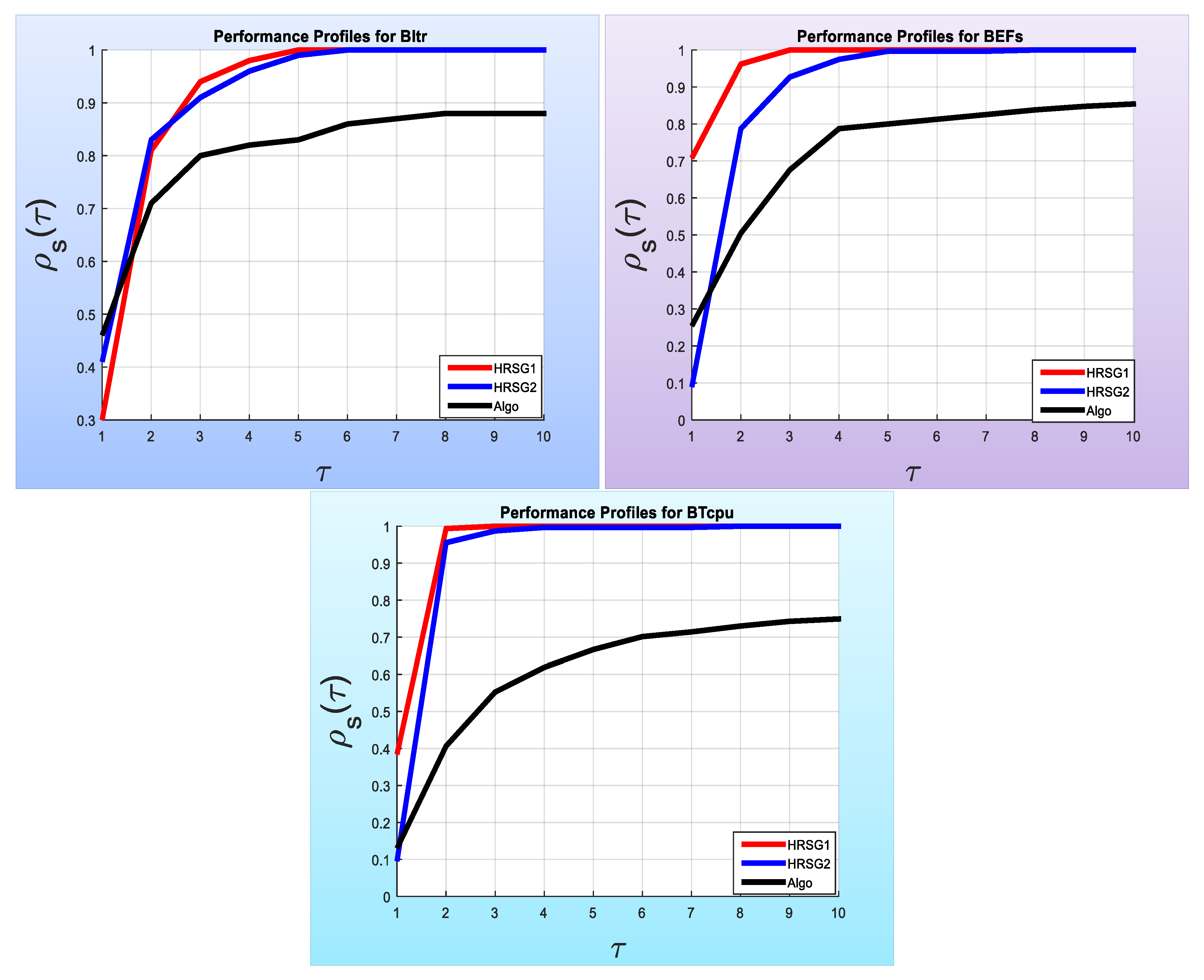
Figure 1 to give an obvious image of the performance of the three algorithms, HRSG1, HRSG2 and Algo. The first graph (left of Figure 1) gives the performance of the BItr for the three algorithms. At τ = 1 , 46 % of test problems were solved by the Algo method against 41 % and 30 % of the test problems solved by the HRSG1 and HRSG2 methods, respectively. This means that the rank of the three algorithms is as follows, Algo algorithm, the HRSG2 algorithm, and HRSG1 algorithm, for the the BItr. When τ = 2 , 83 % of test problems were solved by the HRSG2 method against 81 % and 70 % of the test problems solved by the HRSG1 and Algo methods, respectively. This means that the rank of the three algorithms is as follows, the HRSG2 algorithm, the HRSG1 algorithm, and the Algo algorithm, for the the BItr.
If τ = 3 , 94 % of the test problems were solved by the HRSG1 method against 91 % and 80 % of the test problems solved by the HRSG2 and Algo methods, respectively. This means that the rank of the three algorithms is as follows, HRSG1, HRSG2, and the Algo algorithm for the BItr.
At τ = 5 , all the test problems were solved by the HRSG1 method against 99 % and 83 % of the test problems solved by the HRSG2 and Algo methods, respectively. This means that the rank of the three algorithms is as follows, HRSG1, HRSG2, and the Algo for the BItr.
Finally, at τ = 10 , all the test problems were solved by the HRSG1 and HRSG2 methods against 88 % of the test problems solved by the Algo method. This means that the Algo method failed to solve 12 % of the test problems. It is worth noting that this failure is indicated by (-) in Table 3 (Table A3 of [46]).
The performance profiles for the BFEs and BTcpu are illustrated by the second and third graphs of Figure 1. Therefore, it is clear that the performance of the HRSG1 algorithm is the best.
Furthermore, the results listed in Table 10, Table 11, Table 12, Table 13, Table 14, Table 15, Table 16, Table 17 and Table 18 are presented in Figure 2 and Figure 3 for the WItr, WFEs and WTcpu, and MEItr, MEFEs and METcpu, respectively.
In general, the performance of the HRSG1 is better than the performance of the HRSG2.
Note: Both our proposed algorithms (HRSG1 and HRSG2) are capable of solving all the test problems at the lowest cost, where the WItr did not exceed 100, the WFEs did not exceed 1000 and the WTcpu did not exceed 10 s; while the Algo algorithm failed to solve 12 % of the test problems, illustrated by (-) in Table 3 (Table A3 of [46]).
Thus, in general, the proposed algorithm (HRSG) is competitive with, and in all cases superior to, the Algo algorithm in terms of efficiency, reliability and effectiveness to find the approximate solution of the test problems of the system of non-linear of equations.

5. Conclusions and Future Work

In this paper, we proposed a new adaptive hybrid two-step-size gradient method to solve large-scale systems of non-linear equations.
The proposed algorithm includes a mix of random and deterministic parameters by which two directions are designed. By simulating the forward difference method the ( α k β k ) step-sizes are generated iteratively. The two search directions possess different trust regions and satisfy the sufficient descent condition. The convergence analysis of the HRSG method was established.
The diversity and multiplicity of the parameters give the proposed algorithm several opportunities to reach the feasible region. Therefore, this was a good action that made the proposed algorithm capable of rapidly approaching the approximate solution of all the test problems at each run.
In general, the numerical results demonstrated that the HRSG method is superior compared to the results obtained by the Algo method.
Several evaluation criteria were used to test the performance of the proposed algorithm, providing a fair assessment of the HRSG method.
The proposed HRSG method is represented by two algorithms, HRSG1 and HRSG2.
It is noteworthy that the performance of the HRSG1 algorithm is more efficiency and effective than the HRSG2 algorithm. This is because of the errors resulting from calculating the step-size h ( 0 , 1 ) n (interval).
The combination of the suggested method with the new line search approach results in a new globally convergent method. This new globally convergent method is capable of dealing with local minimization problems. Therefore, when any meta-heuristic technique as a global optimization algorithm is combined with the HRSG as a globally convergent method, the result is a new hybrid semi-gradient meta-heuristic algorithm. The idea behind this hybridization is to utilize the advantages of both techniques. Therefore, the implementation of this idea will be our interest in future work.
Furthermore, the result of this hybridization is a new hybrid semi-gradient meta-heuristic algorithm, capable of dealing with unconstrained, constrained, and multi-objective optimization problems.
It is also attractive to modify and adapt the HRSG method to make it capable of dealing with image restoration problems.
Moreover, it is possible to hybridise the HRSG method with new versions of the CG method. As a result, we could obtain a new hybrid method, capable of training deep neural networks.
The idea of the HRSG method depends on imitating the forward difference method by using one point to estimate the values of the gradient vector at each iteration, where the function evaluation is, at most, one per iteration. Therefore, the HRSG method contains two approaches used to implement this task, namely HRSG1 and HRSG2. Therefore, in future work, both approaches can be used by using the forward and central differences with more than one point.
Furthermore, the approximate values of the gradient vectors can be calculated using the forward and central differences randomly in this case, where the number of function evaluations is zero.
Hence, the proposed method obtained from the above proposals can be applied to deal with systems of non-linear equations, unconstrained, constrained, and multi-objective optimization problems, image restoration, and training deep neural networks.

List of Test Problems

Problem 1: Exponential Function [27,46].
F 1 = e x p ( x 1 ) 1 ,
F i = e x p ( x i ) + x i 1 , i = 2 , 3 , , n
Problem 2: Exponential Function.
F i = l n ( x i + 1 ) x i n , i = 1 , 2 , 3 , , n .
Problem 3: Non-Smooth Function [27,46].
F i = 2 x i s i n ( | x i | ) , i = 1 , 2 , 3 , , n .
Problem 4: [27,46].
F i = min min { | x i | , x i 2 } , max { | x i | , x i 3 } , i = 1 , 2 , 3 , , n .
Problem 5: Strictly Convex Function I [27,46].
F i = e x p ( x i ) 1 , i = 1 , 2 , 3 , , n .
Problem 6: Strictly Convex Function II [46].
F i = i n e x p ( x i ) 1 , i = 1 , 2 , 3 , , n .
Problem 7: Tri-Diagonal Exponential Function [27,46].
F 1 = x 1 e x p ( c o s ( h ( x 1 + x 2 ) ) ,
F i = x i e x p ( c o s ( h ( x i 1 + x i + x i + 1 ) ) , i = 2 , 3 , , n 1 ,
F n = x n e x p ( c o s ( h ( x n 1 + x n ) ) ,
where h = 1 n + 1 .
Problem 8: Non-Smooth Function [27,46].
F i = x i s i n ( | x i 1 | ) , i = 1 , 2 , 3 , , n .
Problem 9: The Trig Exponential Function [27].
F 1 = 3 x 1 3 + 2 x 2 5 + s i n ( x 1 x 2 ) s i n ( x 1 + x 2 ) ,
F i = 3 x i 3 + 2 x i + 1 5 + s i n ( x i x i + 1 ) s i n ( x i + x i + 1 ) + 4 x i x i 1 e x p ( x i 1 x i ) 3 , i = 2 , 3 , , n 1 .
F n = x n 1 e x p ( x n 1 x n ) + 4 x n 3 .
Initial Points (INP):  x 1 = ( 0.1 , 0.1 , , 0.1 ) , x 2 = ( 0.2 , 0.2 , , 0.2 ) , x 3 = ( 0.5 , 0.5 , , 0.5 ) , x 4 = ( 1.2 , 1.2 , , 1.2 ) , x 5 = ( 1.5 , 1.5 , , 1.5 ) , x 6 = ( 2 , 2 , , 2 ) and x 7 = rand ( n , 1 ) .

Author Contributions

Conceptualization, E.A.; methodology, E.A. and S.M.; software, E.A. and S.M.; validation, E.A.; formal analysis, E.A.; investigation, E.A.; Funding acquisition, E.A.; data curation, E.A.; writing original draft preparation, E.A. and S.M.; writing-review and editing E.A. and S.M.; visualization, E.A. and S.M.; supervision, E.A. and S.M. All authors have read and agreed to the published version of the manuscript.

Funding

This research was funded by the Deanship of Scientific Research at Najran University (grant number NU/DRP/SERC/12/3).

Data Availability Statement

Not applicable.

Acknowledgments

The authors are thankful to the Deanship of Scientific Research at Najran University for funding this work, under the General Research Funding program grant code (NU/DRP/SERC/12/3).

Conflicts of Interest

The authors declare no conflict of interest.

References

  1. Alnowibet, K.A.; Alshamrani, A.M.; Alrasheedi, A.F.; Mahdi, S.; El-Alem, M.; Aboutahoun, A.; Mohamed, A.W. Efficient Modified Meta-Heuristic Technique for Unconstrained Optimization Problems. Axioms 2022, 11, 483. [Google Scholar] [CrossRef]
  2. Abubakar, A.B.; Kumam, P.; Mohammad, H.; Ibrahim, A.H.; Kiri, A.I. A hybrid approach for finding approximate solutions to constrained nonlinear monotone operator equations with applications. Appl. Numer. Math. 2022, 177, 79–92. [Google Scholar] [CrossRef]
  3. Meintjes, K.; Morgan, A.P. Chemical equilibrium systems as numerical test problems. ACM Trans. Math. Softw. (TOMS) 1990, 16, 143–151. [Google Scholar] [CrossRef]
  4. Xiao, Y.; Zhu, H. A conjugate gradient method to solve convex constrained monotone equations with applications in compressive sensing. J. Math. Anal. Appl. 2013, 405, 310–319. [Google Scholar] [CrossRef]
  5. Abubakar, A.B.; Mohammad, H.; Kumam, P.; Rano, S.A.; Ibrahim, A.H.; Kiri, A.I. On the new spectral conjugate gradient-type method for monotone nonlinear equations and signal recovery. Math. Methods Appl. Sci. 2022. [Google Scholar] [CrossRef]
  6. Ibrahim, A.H.; Kumam, P.; Abubakar, A.B.; Abdullahi, M.S.; Mohammad, H. A Dai-Liao-type projection method for monotone nonlinear equations and signal processing. Demonstr. Math. 2022, 55, 978–1013. [Google Scholar] [CrossRef]
  7. Brown, P.N.; Saad, Y. Convergence theory of nonlinear Newton–Krylov algorithms. SIAM J. Optim. 1994, 4, 297–330. [Google Scholar] [CrossRef]
  8. Li, D.H.; Fukushima, M. A modified BFGS method and its global convergence in nonconvex minimization. J. Comput. Appl. Math. 2001, 129, 15–35. [Google Scholar] [CrossRef]
  9. Fletcher, R.; Reeves, C.M. Function minimization by conjugate gradients. Comput. J. 1964, 7, 149–154. [Google Scholar] [CrossRef]
  10. Hestenes, M.R.; Stiefel, E. Methods of Conjugate Gradients for Solving. J. Res. Natl. Bur. Stand. 1952, 49, 409. [Google Scholar] [CrossRef]
  11. Liu, Y.; Storey, C. Efficient generalized conjugate gradient algorithms, part 1: Theory. J. Optim. Theory Appl. 1991, 69, 129–137. [Google Scholar] [CrossRef]
  12. Polak, E.; Ribiere, G. Note sur la convergence de méthodes de directions conjuguées. ESAIM Math. Model. Numer. Anal. Model. Math. Anal. Numer. 1969, 3, 35–43. [Google Scholar] [CrossRef]
  13. Birgin, E.G.; Krejić, N.; Martínez, J.M. Globally convergent inexact quasi-Newton methods for solving nonlinear systems. Numer. Algorithms 2003, 32, 249–260. [Google Scholar] [CrossRef]
  14. Li, D.; Fukushima, M. A globally and superlinearly convergent gauss–Newton-based BFGS method for symmetric nonlinear equations. SIAM J. Numer. Anal. 1999, 37, 152–172. [Google Scholar] [CrossRef]
  15. Li, D.H.; Fukushima, M. A derivative-free line search and global convergence of Broyden-like method for nonlinear equations. Optim. Methods Softw. 2000, 13, 181–201. [Google Scholar] [CrossRef]
  16. Solodov, M.V.; Svaiter, B.F. A globally convergent inexact Newton method for systems of monotone equations. In Reformulation: Nonsmooth, Piecewise Smooth, Semismooth and Smoothing Methods; Springer: Cham, Switzerland, 1998; pp. 355–369. [Google Scholar]
  17. Zhou, G.; Toh, K.C. Superlinear convergence of a Newton-type algorithm for monotone equations. J. Optim. Theory Appl. 2005, 125, 205–221. [Google Scholar] [CrossRef]
  18. Abubakar, A.B.; Kumam, P. A descent Dai-Liao conjugate gradient method for nonlinear equations. Numer. Algorithms 2019, 81, 197–210. [Google Scholar] [CrossRef]
  19. Dai, Z.; Zhu, H. A modified Hestenes-Stiefel-type derivative-free method for large-scale nonlinear monotone equations. Mathematics 2020, 8, 168. [Google Scholar] [CrossRef]
  20. Su, Z.; Li, M. A Derivative-Free Liu–Storey Method for Solving Large-Scale Nonlinear Systems of Equations. Math. Probl. Eng. 2020, 2020, 6854501. [Google Scholar] [CrossRef]
  21. Yuan, G.; Wei, Z.; Lu, S. Limited memory BFGS method with backtracking for symmetric nonlinear equations. Math. Comput. Model. 2011, 54, 367–377. [Google Scholar] [CrossRef]
  22. Yuan, G.; Li, T.; Hu, W. A conjugate gradient algorithm for large-scale nonlinear equations and image restoration problems. Appl. Numer. Math. 2020, 147, 129–141. [Google Scholar] [CrossRef]
  23. Zhang, L.; Zhou, W. Spectral gradient projection method for solving nonlinear monotone equations. J. Comput. Appl. Math. 2006, 196, 478–484. [Google Scholar] [CrossRef]
  24. Ibrahim, A.H.; Deepho, J.; Abubakar, A.B.; Kamandi, A. A globally convergent derivative-free projection algorithm for signal processing. J. Interdiscip. Math. 2022, 25, 2301–2320. [Google Scholar] [CrossRef]
  25. Cruz, W.L. A spectral algorithm for large-scale systems of nonlinear monotone equations. Numer. Algorithms 2017, 76, 1109–1130. [Google Scholar] [CrossRef]
  26. Dennis, J.E.; Moré, J.J. A characterization of superlinear convergence and its application to quasi-Newton methods. Math. Comput. 1974, 28, 549–560. [Google Scholar] [CrossRef]
  27. Stanimirovic, P.S.; Shaini, B.I.; Sabiu, J.; Shah, A.; Petrovic, M.J.; Ivanov, B.; Cao, X.; Stupina, A.; Li, S. Improved Gradient Descent Iterations for Solving Systems of Nonlinear Equations. Algorithms 2023, 16, 64. [Google Scholar] [CrossRef]
  28. Waziri, M.Y.; Muhammad, H.U.; Halilu, A.S.; Ahmed, K. Modified matrix-free methods for solving system of nonlinear equations. Optimization 2021, 70, 2321–2340. [Google Scholar] [CrossRef]
  29. Kumam, P.; Abubakar, A.B.; Ibrahim, A.H.; Kura, H.U.; Panyanak, B.; Pakkaranang, N. Another hybrid approach for solving monotone operator equations and application to signal processing. Math. Methods Appl. Sci. 2022, 45, 7897–7922. [Google Scholar] [CrossRef]
  30. Dai, Z.; Wen, F. Global convergence of a modified Hestenes-Stiefel nonlinear conjugate gradient method with Armijo line search. Numer. Algorithms 2012, 59, 79–93. [Google Scholar] [CrossRef]
  31. Ibrahim, A.H.; Kumam, P.; Abubakar, A.B.; Abubakar, J. A derivative-free projection method for nonlinear equations with non-Lipschitz operator: Application to LASSO problem. Math. Methods Appl. Sci. 2023. [Google Scholar] [CrossRef]
  32. Alnowibet, K.A.; Mahdi, S.; El-Alem, M.; Abdelawwad, M.; Mohamed, A.W. Guided Hybrid Modified Simulated Annealing Algorithm for Solving Constrained Global Optimization Problems. Mathematics 2022, 10, 1312. [Google Scholar] [CrossRef]
  33. EL-Alem, M.; Aboutahoun, A.; Mahdi, S. Hybrid gradient simulated annealing algorithm for finding the global optimal of a nonlinear unconstrained optimization problem. Soft Comput. 2020, 25, 2325–2350. [Google Scholar] [CrossRef]
  34. Kramer, O.; Ciaurri, D.E.; Koziel, S. Derivative-free optimization. In Computational Optimization, Methods and Algorithms; Springer: Cham, Switzerland, 2011; pp. 61–83. [Google Scholar]
  35. Larson, J.; Menickelly, M.; Wild, S.M. Derivative-free optimization methods. Acta Numer. 2019, 28, 287–404. [Google Scholar] [CrossRef]
  36. Shi, H.J.M.; Xie, Y.; Xuan, M.Q.; Nocedal, J. Adaptive Finite-Difference Interval Estimation for Noisy Derivative-Free Optimization. arXiv 2021, arXiv:2110.06380. [Google Scholar] [CrossRef]
  37. Shi, H.J.M.; Xuan, M.Q.; Oztoprak, F.; Nocedal, J. On the numerical performance of derivative-free optimization methods based on finite-difference approximations. arXiv 2021, arXiv:2102.09762. [Google Scholar]
  38. Berahas, A.S.; Cao, L.; Choromanski, K.; Scheinberg, K. A theoretical and empirical comparison of gradient approximations in derivative-free optimization. Found. Comput. Math. 2022, 22, 507–560. [Google Scholar] [CrossRef]
  39. Curtis, A.; Reid, J. The choice of step lengths when using differences to approximate Jacobian matrices. IMA J. Appl. Math. 1974, 13, 121–126. [Google Scholar] [CrossRef]
  40. Frontini, M.; Milovanović, G.V. Numerical differentiation of analytic functions using quadratures on the semicircle. Comput. Math. Appl. 1991, 22, 99–106. [Google Scholar]
  41. Gill, P.E.; Murray, W.; Saunders, M.A.; Wright, M.H. Computing forward-difference intervals for numerical optimization. SIAM J. Sci. Stat. Comput. 1983, 4, 310–321. [Google Scholar] [CrossRef]
  42. Xie, Y. Methods for Nonlinear and Noisy Optimization. Ph.D. Thesis, Northwestern University, Evanston, IL, USA, 2021. [Google Scholar]
  43. Alnowibet, K.A.; Mahdi, S.; Alshamrani, A.M.; Sallam, K.M.; Mohamed, A.W. A Family of Hybrid Stochastic Conjugate Gradient Algorithms for Local and Global Minimization Problems. Mathematics 2022, 10, 3595. [Google Scholar] [CrossRef]
  44. Alshamrani, A.M.; Alrasheedi, A.F.; Alnowibet, K.A.; Mahdi, S.; Mohamed, A.W. A Hybrid Stochastic Deterministic Algorithm for Solving Unconstrained Optimization Problems. Mathematics 2022, 10, 3032. [Google Scholar] [CrossRef]
  45. Conn, A.R.; Scheinberg, K.; Vicente, L.N. Introduction to Derivative-Free Optimization; SIAM: Philadelphia, PA, USA, 2009. [Google Scholar]
  46. Hassan Ibrahim, A.; Kumam, P.; Hassan, B.A.; Bala Abubakar, A.; Abubakar, J. A derivative-free three-term Hestenes–Stiefel type method for constrained nonlinear equations and image restoration. Int. J. Comput. Math. 2022, 99, 1041–1065. [Google Scholar] [CrossRef]
  47. Ali, M.M.; Khompatraporn, C.; Zabinsky, Z.B. A numerical evaluation of several stochastic algorithms on selected continuous global optimization test problems. J. Glob. Optim. 2005, 31, 635–672. [Google Scholar] [CrossRef]
  48. Barbosa, H.J.; Bernardino, H.S.; Barreto, A.M. Using performance profiles to analyze the results of the 2006 CEC constrained optimization competition. In Proceedings of the IEEE Congress on Evolutionary Computation, Barcelona, Spain, 18–23 July 2010; pp. 1–8. [Google Scholar]
  49. Dolan, E.D.; Moré, J.J. Benchmarking optimization software with performance profiles. Math. Program. 2002, 91, 201–213. [Google Scholar] [CrossRef]
  50. Moré, J.J.; Wild, S.M. Benchmarking derivative-free optimization algorithms. SIAM J. Optim. 2009, 20, 172–191. [Google Scholar] [CrossRef]
  51. Vaz, A.I.F.; Vicente, L.N. A particle swarm pattern search method for bound constrained global optimization. J. Glob. Optim. 2007, 39, 197–219. [Google Scholar] [CrossRef]
Figure 1. The BItr, BEFs, and BTcpu obtained by the HRSG1, HRSG2 and Algo methods.
Mathematics 11 02102 g001
Figure 2. The WItr, WFEs and WTcpu obtained by the HRSG1 and HRSG2 methods.
Mathematics 11 02102 g002
Figure 3. The MEItr, MEFEs and METcpu obtained by the HRSG1 and HRSG2 methods.
Mathematics 11 02102 g003aMathematics 11 02102 g003b
Table 1. Numeral results (Problem 1) for the terms BItr, BEFs and BTcpu of the three methods.
nINPHRSG1HRSG2Algo
BItrBEFsBTcpuBItrBEFsBTcpuBItrBEFsBTcpu
1000 x 1 6120.0026180.002270.015
x 2 6120.0027210.003270.009
x 3 7140.0027210.004270.021
x 4 6120.0027210.003270.009
x 5 9180.0038240.003270.013
x 6 6120.0029270.004270.007
x 7 7140.0028240.0038320.010
5000 x 1 5100.0067210.009270.016
x 2 6120.0067210.009270.023
x 3 5100.0058240.010270.021
x 4 7140.0088240.012270.018
x 5 8160.0099270.012270.017
x 6 8160.0099270.013270.018
x 7 7140.0086180.0088320.029
10,000 x 1 6120.0138240.022270.033
x 2 6120.0138240.021270.021
x 3 8160.0176180.016270.027
x 4 7140.0157210.018270.021
x 5 9180.01910300.027270.029
x 6 7140.0159270.023270.028
x 7 6120.0138240.0218320.049
50,000 x 1 5100.0598240.116270.083
x 2 7140.0827210.104270.082
x 3 9180.1056180.086270.134
x 4 6120.07210300.142270.096
x 5 7140.0858240.113270.108
x 6 9180.10710300.142270.097
x 7 7140.0838240.1288320.218
100,000 x 1 7140.1848240.250270.160
x 2 8160.2289270.304270.164
x 3 8160.2398240.256270.158
x 4 7140.21511330.353270.161
x 5 9180.23910300.323270.175
x 6 8160.21711330.392270.185
x 7 7140.1869270.3199360.393
Table 2. Numeral results (Problem 2) for the terms BItr, BEFs and BTcpu for the three methods.
nINPHRSG1HRSG2Algo
BItrBEFsBTcpuBItrBEFsBTcpuBItrBEFsBTcpu
1000 x 1 480.0014120.0026190.012
x 2 480.0014120.0026190.006
x 3 5100.002390.0016190.006
x 4 6120.0025150.0027220.005
x 5 5100.0024120.0026190.007
x 6 6120.002390.0018250.005
x 7 480.0015150.00215490.017
5000 x 1 5100.0064120.0066200.015
x 2 480.0044120.0066200.021
x 3 5100.0054120.0066190.014
x 4 6120.0075150.0077230.021
x 5 5100.006390.0066190.016
x 6 5100.0064120.0078250.019
x 7 5100.005390.00715500.042
10,000 x 1 480.0094120.0146200.032
x 2 5100.0124120.0136200.028
x 3 480.0095150.0146190.031
x 4 480.009390.0087230.034
x 5 5100.0124120.0126190.029
x 6 6120.014390.0088260.036
x 7 5100.0126180.01613440.066
50,000 x 1 5100.0604120.0636200.097
x 2 480.0484120.0566200.095
x 3 5100.0594120.0797230.119
x 4 5100.0624120.0587230.123
x 5 5100.0604120.0707230.179
x 6 6120.0725150.0738260.151
x 7 5100.0614120.06415510.300
100,000 x 1 5100.1445150.1786200.215
x 2 480.115390.1347250.229
x 3 480.1194120.1357240.261
x 4 6120.1736180.2118280.288
x 5 6120.1725150.1687230.225
x 6 480.1184120.1358260.258
x 7 5100.1535150.16915510.851
Table 3. Numeral results (Problem 3) for the terms BItr, BEFs and BTcpu for the three methods.
nINPHRSG1HRSG2Algo
BItrBEFsBTcpuBItrBEFsBTcpuBItrBEFsBTcpu
1000 x 1 5100.002390.0027270.006
x 2 6120.0025150.0027280.007
x 3 5100.002390.0026240.007
x 4 6120.002390.001---
x 5 6120.0026180.002---
x 6 6120.0026180.002---
x 7 5100.0015150.002---
5000 x 1 5100.0055150.0077280.013
x 2 480.0044120.0088310.017
x 3 5100.0055150.0067270.013
x 4 6120.0066180.008---
x 5 7140.0074120.005---
x 6 5100.0056180.0078320.017
x 7 5100.0056180.008---
10,000 x 1 5100.0115150.0127270.025
x 2 5100.0114120.0138320.028
x 3 5100.0106180.0157270.025
x 4 7140.0156180.017---
x 5 6120.0135150.012---
x 6 5100.0105150.0168320.031
x 7 7140.0156180.015---
50,000 x 1 6120.0686180.0898320.117
x 2 6120.0665150.0617270.094
x 3 6120.0675150.0626230.080
x 4 6120.0667210.087---
x 5 5100.0547210.097---
x 6 6120.0757210.1038310.112
x 7 7140.0777210.118---
100,000 x 1 360.0725150.1507270.175
x 2 7140.1664120.1198310.241
x 3 8160.1956180.1798320.261
x 4 6120.1564120.136---
x 5 7140.1908240.241---
x 6 7140.1878240.2399360.253
x 7 7140.1917210.213---
Table 4. Numeral results (Problem 4) for the terms BItr, BEFs and BTcpu for the three methods.
nINPHRSG1HRSG2Algo
BItrBEFsBTcpuBItrBEFsBTcpuBItrBEFsBTcpu
1000 x 1 240.001390.004260.006
x 2 360.002260.002260.004
x 3 360.0024120.005260.005
x 4 360.0025150.005270.005
x 5 240.002130.001270.009
x 6 480.0035150.005270.005
x 7 5100.0044120.00425800.021
5000 x 1 360.0074120.011260.019
x 2 5100.0115150.015260.017
x 3 480.0094120.011260.019
x 4 480.0094120.011270.020
x 5 360.007130.004270.019
x 6 120.002390.009270.016
x 7 480.009130.00325790.103
10,000 x 1 480.017260.011260.029
x 2 480.016390.022260.023
x 3 480.014390.016260.025
x 4 360.0114120.022270.024
x 5 480.015260.011270.027
x 6 5100.022390.017270.022
x 7 5100.0196180.03327850.199
50,000 x 1 5100.093390.109260.096
x 2 5100.0934120.114260.097
x 3 240.0374120.110260.100
x 4 6120.127260.100270.095
x 5 120.021130.028270.093
x 6 5100.104390.082270.096
x 7 5100.1055150.14229890.839
100,000 x 1 480.1764120.227260.192
x 2 360.1204120.228260.213
x 3 360.129390.175260.197
x 4 480.169390.172270.187
x 5 240.0894120.321270.189
x 6 120.0405150.286270.196
x 7 480.1804120.23429911.666
Table 5. Numeral results (Problem 5) for the terms BItr, BEFs and BTcpu for the three methods.
nINPHRSG1HRSG2Algo
BItrBEFsBTcpuBItrBEFsBTcpuBItrBEFsBTcpu
1000 x 1 480.0015150.002270.004
x 2 6120.002390.001270.004
x 3 5100.0025150.0027280.005
x 4 6120.0024120.002270.006
x 5 6120.0024120.002270.004
x 6 5100.0025150.002270.004
x 7 6120.0024120.00221840.024
5000 x 1 480.005390.005270.014
x 2 360.0045150.008270.014
x 3 5100.0065150.0078320.018
x 4 6120.0076180.009270.018
x 5 480.0055150.007270.016
x 6 5100.0064120.006270.015
x 7 5100.006390.005411630.160
10,000 x 1 5100.011390.008270.023
x 2 480.0094120.011270.019
x 3 6120.0144120.0118320.024
x 4 5100.0125150.014270.019
x 5 5100.0125150.015270.018
x 6 5100.0125150.014270.025
x 7 5100.012390.009361440.228
50,000 x 1 360.0364120.057270.069
x 2 480.052390.043270.069
x 3 6120.0715150.0688320.092
x 4 6120.0725150.068270.095
x 5 6120.0735150.068270.079
x 6 6120.0735150.067270.083
x 7 5100.0615150.068682712.160
100,000 x 1 5100.1285150.153270.130
x 2 480.1134120.128270.131
x 3 5100.1295150.1489360.205
x 4 6120.1544120.1209360.207
x 5 5100.1215150.155270.144
x 6 6120.1445150.149270.168
x 7 480.0975150.1481064246.702
Table 6. Numeral results (Problem 6) for the terms BItr, BEFs and BTcpu for the three methods.
nINPHRSG1HRSG2Algo
BItrBEFsBTcpuBItrBEFsBTcpuBItrBEFsBTcpu
1000 x 1 7140.0026180.00317640.009
x 2 8160.0035150.00218680.013
x 3 7140.00310300.005261010.016
x 4 9180.0036180.003271080.020
x 5 8160.0038240.004311240.030
x 6 9180.0046180.003753000.096
x 7 360.0018240.004582280.045
5000 x 1 6120.0078240.012301150.098
x 2 6120.0076180.01025960.064
x 3 6120.0079270.013411590.140
x 4 10200.0128240.012421670.158
x 5 5100.0068240.012582300.247
x 6 8160.0095150.011883520.595
x 7 7140.0098240.014893550.425
10,000 x 1 8160.01910300.029271030.126
x 2 7140.0165150.01525960.122
x 3 8160.0188240.023451760.269
x 4 10200.02310300.032632520.526
x 5 8160.0186180.017833320.803
x 6 5100.0116180.0181254991.281
x 7 8160.01810300.0271214831.147
50,000 x 1 5100.0579270.114351350.689
x 2 5100.0628240.104341320.712
x 3 11220.1369270.117803172.568
x 4 8160.1029270.1301124484.068
x 5 7140.09511330.1571204794.810
x 6 10200.1279270.12620581810.627
x 7 7140.08811330.1561987918.100
100,000 x 1 8160.2167210.213401551.715
x 2 9180.24410300.302481862.175
x 3 7140.1748240.246883495.323
x 4 5100.1258240.222873485.862
x 5 6120.16211330.30214557912.157
x 6 11220.2979270.27922489621.001
x 7 10200.2689270.27119376815.277
Table 7. Numeral results (Problem 7) for the terms BItr, BEFs and BTcpu for the three methods.
nINPHRSG1HRSG2Algo
BItrBEFsBTcpuBItrBEFsBTcpuBItrBEFsBTcpu
1000 x 1 25500.01424720.01613520.019
x 2 25500.01324770.01713520.011
x 3 23460.01223720.01613520.014
x 4 25500.01422680.01612480.013
x 5 23460.01223690.01512480.015
x 6 25510.01421650.01512480.013
x 7 30600.01628860.01913520.014
5000 x 1 26520.04422720.04813520.044
x 2 24480.04025760.05113520.051
x 3 22440.03723730.04713520.051
x 4 23460.03822680.04413520.045
x 5 24480.04023690.05213520.044
x 6 26520.04322710.04613520.044
x 7 29580.05130940.06213520.049
10,000 x 1 24480.07623710.08514560.083
x 2 24480.08024720.08614560.081
x 3 24480.07223720.08613520.076
x 4 24480.07621660.07913520.074
x 5 24480.07421690.08413520.082
x 6 23460.07123770.09113520.071
x 7 30600.08331970.12513520.077
50,000 x 1 26520.34823710.41414560.332
x 2 24480.32324750.43314560.340
x 3 25500.36423710.40714560.413
x 4 23470.34425770.43814560.312
x 5 23460.34023720.41414560.327
x 6 24480.37022690.39413520.314
x 7 32640.442331060.61114560.361
100,000 x 1 24480.75025780.88914560.704
x 2 24480.78323720.88814560.701
x 3 23460.68521670.83414560.702
x 4 25510.79922670.85514560.690
x 5 22440.72023720.91514560.708
x 6 26520.84322700.87813520.659
x 7 34681.08530991.23514560.712
Table 8. Numeral results (Problem 8) for the terms BItr, BEFs and BTcpu for the three methods.
nINPHRSG1HRSG2Algo
BItrBEFsBTcpuBItrBEFsBTcpuBItrBEFsBTcpu
1000 x 1 10200.00613390.0087280.009
x 2 10200.00612360.0077280.006
x 3 7140.00410300.0066240.006
x 4 10200.00610300.0067280.006
x 5 10200.00812360.0077280.009
x 6 9180.00512360.0078310.007
x 7 10200.00610300.00611440.009
5000 x 1 10200.0179270.0177280.018
x 2 8160.0139270.0177280.017
x 3 8160.0137210.0146240.017
x 4 9180.01614420.0258320.022
x 5 12240.02210300.0198320.023
x 6 14280.02510300.0198310.033
x 7 13260.02312360.02711440.030
10,000 x 1 9180.02811330.0398320.032
x 2 11220.0367210.0247280.044
x 3 9180.0299270.0316240.035
x 4 11220.03713390.0408320.035
x 5 8160.02511330.0338320.034
x 6 12240.04210300.0318310.039
x 7 10200.03010300.03311440.054
50,000 x 1 13260.18213390.1788320.135
x 2 13260.19812360.1648320.170
x 3 11220.17110300.1417280.114
x 4 11220.15810300.1538320.202
x 5 12240.19811330.1978320.163
x 6 11220.15512360.1849350.139
x 7 14280.19812360.18612480.232
100,000 x 1 13260.39012360.3838320.258
x 2 13260.38411330.3538320.263
x 3 8160.2408240.2887280.236
x 4 12240.38612360.3828320.295
x 5 13260.39513390.4218320.258
x 6 16320.48113390.3819350.321
x 7 12240.36211330.35612480.439
Table 9. Numeral results (Problem 9) for the terms BItr, BEFs and BTcpu for the three methods.
nINPHRSG1HRSG2Algo
BItrBEFsBTcpuBItrBEFsBTcpuBItrBEFsBTcpu
1000 x 1 21520.03723800.043431720.213
x 2 22560.03921760.044451800.251
x 3 23580.04022800.046461840.232
x 4 23590.04122780.044461840.241
x 5 24570.04123860.046361440.205
x 6 23560.04724880.047491960.274
x 7 24630.04523840.046461840.252
5000 x 1 23570.09222810.108451801.089
x 2 23580.09723820.108451801.176
x 3 22560.09122770.106421681.020
x 4 22560.09023800.109411640.981
x 5 23570.09821770.103431721.134
x 6 24590.09823840.112461841.229
x 7 23610.10222820.109441761.221
10,000 x 1 23570.15924840.202451802.202
x 2 23580.16322790.188451802.004
x 3 22550.15722800.191451802.012
x 4 22570.15722770.186381521.797
x 5 23550.15623810.196431721.957
x 6 23590.16522810.192451802.340
x 7 23620.17224880.212451802.332
50,000 x 1 23580.74122800.898481928.885
x 2 21560.70723830.958471889.060
x 3 22580.70423820.914441769.092
x 4 20510.63021750.856421688.086
x 5 22550.68321750.925401607.622
x 6 23590.71924860.9834919610.299
x 7 24570.76423860.983441769.279
100,000 x 1 22591.49422781.8514819219.169
x 2 22571.47822781.8214718819.064
x 3 22571.45622821.8925522021.406
x 4 23601.52422801.8494317215.747
x 5 22581.46622821.8954317216.544
x 6 24601.53922811.9475220826.298
x 7 24651.74723862.0624518019.981
Table 10. Numeral results (Problem 1) for the terms WItr, WEFs and WTcpu for the three methods.
nINPHRSG1HRSG2HRSG1HRSG2
WItrWEFsWTcpuWItrWEFsWTcpuMEtrMEEFsMETcpuMEItrMEEFsMETcpu
1000 x 1 12240.00515450.1288.817.60.00310.631.80.012
x 2 12240.00416480.0068.9517.90.00310.9532.850.004
x 3 12240.00418540.0079.7519.50.00312.2536.750.005
x 4 16320.00518550.0089.9519.90.00312.2536.80.005
x 5 15300.00517510.00710.8521.70.00312.236.60.005
x 6 15300.00518540.00710.8521.70.00314.142.30.005
x 7 13260.00417510.0079.3518.70.00312.738.10.005
5000 x 1 12240.01414420.0528.5170.01011.233.60.019
x 2 12240.01419570.0268.5517.10.01011.4534.350.016
x 3 12240.01316480.0218.8517.70.01011.1533.450.015
x 4 13260.01417510.02310.1520.30.01113.2539.750.018
x 5 14280.01617510.02410.420.80.01213.0539.150.018
x 6 13260.01520600.02810.6521.30.01214.1542.450.020
x 7 13260.02517510.02310.1520.30.01211.735.10.017
10,000 x 1 12240.02618540.0538.617.20.01911.735.10.032
x 2 13260.02918540.0479.418.80.02112.3537.050.034
x 3 13260.03019570.05110.1520.30.02311.9535.850.032
x 4 14280.03021630.05610.220.40.02212.938.70.034
x 5 14280.03220610.05611220.02413.65410.037
x 6 14280.03120600.05310.1520.30.02313.741.10.037
x 7 13260.03518540.0489.4518.90.02112.5537.650.034
50,000 x 1 11220.13917510.2738.917.80.10611.534.50.177
x 2 14280.16719570.31310.120.20.12012.0536.150.183
x 3 14280.16618540.25510.3520.70.12212.3537.050.177
x 4 15300.17820600.28310.5521.10.12513.9541.850.200
x 5 16320.18818540.26010.821.60.12813.741.10.197
x 6 14280.16717510.24511.723.40.13914420.201
x 7 12240.14817510.27110.420.80.12413.0539.150.191
100,000 x 1 12240.31316480.5929.8519.70.26411.8535.550.386
x 2 12240.33519570.66510.120.20.27813.440.20.455
x 3 12240.34519570.66810.4520.90.28814.4543.350.485
x 4 15300.42120600.68211.322.60.32215.245.60.533
x 5 16320.43318540.70011.823.60.31414.1542.450.510
x 6 14280.37119570.83711.422.80.30215.546.50.606
x 7 12240.32215450.64810.2520.50.27212.5537.650.471
Table 11. Numeral results (Problem 2) for the terms WItr, WEFs and WTcpu for the three methods.
nINPHRSG1HRSG2HRSG1HRSG2
WItrWEFsWTcpuWItrWEFsWTcpuMEtrMEEFsMETcpuMEItrMEEFsMETcpu
1000 x 1 8160.0038270.0096.3512.70.0026.118.30.003
x 2 8160.0039270.0056.813.60.0026.218.60.003
x 3 10200.0039270.0057.2514.50.0026.519.50.003
x 4 9180.0039270.0056.9513.90.0026.8520.550.003
x 5 10200.0049270.0057.5515.10.0037210.004
x 6 11220.0049240.0057.5150.0036.1518.450.003
x 7 10200.0038240.0046.813.60.0026.4519.350.003
5000 x 1 10200.0128270.0147140.0086.419.20.011
x 2 9180.0119300.0156.713.40.0086.2518.750.010
x 3 10200.01110270.0167.0514.10.0087.321.90.012
x 4 11220.0129240.0168.0516.10.0096.619.80.011
x 5 11220.0128300.0247.7515.50.0096.5519.650.015
x 6 12240.01310270.0167.4514.90.0087.0521.150.012
x 7 10200.0129240.0187.414.80.0096.8520.550.013
10,000 x 1 9180.0208270.0366.8513.70.0156.218.60.023
x 2 10200.0349270.0387.915.80.0196.920.70.024
x 3 12240.0309270.0277.715.40.0186.720.10.019
x 4 11220.0249300.0257.9515.90.0186.5519.650.018
x 5 11220.02810270.0297.6515.30.0197.1521.450.020
x 6 13260.0299270.0258.216.40.0196.419.20.018
x 7 11220.0259300.0277.2514.50.0177.0521.150.020
50,000 x 1 10200.12610300.1416.9513.90.0946.519.50.100
x 2 11220.16610270.1427.214.40.0927.121.30.103
x 3 10200.1219300.1697.114.20.0886.820.40.106
x 4 11220.13510270.1857.915.80.0967210.115
x 5 11220.1339270.2148.5170.1036.4519.350.123
x 6 10200.1229270.1748.0516.10.0987.3522.050.120
x 7 11220.1499240.2897.915.80.1036.3519.050.132
100,000 x 1 10200.2878270.3857.3514.70.2186.519.50.249
x 2 11220.3339270.3617.0514.10.2066.6519.950.252
x 3 10200.3209300.3257.815.60.2317.221.60.251
x 4 13260.37410300.4008.717.40.2517.4522.350.283
x 5 13260.37510270.3648.5517.10.2467.4522.350.262
x 6 11220.3769300.3338.7517.50.2676.7520.250.239
x 7 10200.32110 0.4308160.2397.622.80.286
Table 12. Numeral results (Problem 3) for the terms WItr, WEFs and WTcpu for the three methods.
nINPHRSG1HRSG2HRSG1HRSG2
WItrWEFsWTcpuWItrWEFsWTcpuMEtrMEEFsMETcpuMEItrMEEFsMETcpu
1000 x 1 12240.005410300.00518.116.20.0037.7523.250.0033
x 2 11220.00311330.00488.617.20.00268.124.30.003
x 3 12240.00412360.0078.6517.30.0038.525.50.004
x 4 13260.00413390.0069.418.80.0038.3525.050.004
x 5 14280.00416480.0079.0518.10.0039.7529.250.004
x 6 14280.00414420.0089.7519.50.0039.7529.250.004
x 7 13260.00411330.0058.917.80.0038.324.90.004
5000 x 1 12240.01211330.0168.216.40.0088.6525.950.013
x 2 11220.01112360.0248.1516.30.0088.324.90.014
x 3 13260.01313390.0229.218.40.0108.6525.950.012
x 4 12240.01214420.0219.1518.30.0099.2527.750.013
x 5 14280.01513390.0179.418.80.01010.230.60.013
x 6 14280.01513390.0199.4518.90.0109.528.50.012
x 7 13260.01413390.0219180.0109.528.50.014
10,000 x 1 11220.02312360.0318.2516.50.0188.5525.650.022
x 2 12240.02613390.0398.817.60.0198.525.50.025
x 3 12240.02513390.0378.617.20.0189.127.30.024
x 4 13260.03013390.0419.819.60.02110300.031
x 5 15300.03216480.0389.819.60.0219.829.40.028
x 6 15300.03214420.04710.1520.30.0229.628.80.028
x 7 15300.03213390.04910.2520.50.0239.7529.250.028
50,000 x 1 12240.14015450.2058.8517.70.09910300.136
x 2 13260.14612360.1719.118.20.1018.3525.050.111
x 3 12240.15114420.17610200.1139.3528.050.119
x 4 14280.15315450.18710.1520.30.11510.531.50.133
x 5 16320.17614420.21810.921.80.1229.729.10.143
x 6 14280.15714420.19611.122.20.12210.631.80.149
x 7 13260.14313390.2249.7519.50.1089.7529.250.157
100,000 x 1 10200.24312360.4227.915.80.1907.823.40.253
x 2 13260.32912360.3589.8519.70.2458.124.30.242
x 3 13260.34512360.4459.619.20.2549.528.50.318
x 4 13260.36513390.59110.1520.30.2719.6528.950.344
x 5 15300.39515450.54610.921.80.30210.832.40.356
x 6 14280.36416480.53610.420.80.28110.3531.050.334
x 7 13260.35012360.43310.420.80.2799.2527.750.306
Table 13. Numeral results (Problem 4) for the terms WItr, WEFs and WTcpu for the three methods.
nINPHRSG1HRSG2HRSG1HRSG2
WItrWEFsWTcpuWItrWEFsWTcpuMEtrMEEFsMETcpuMEItrMEEFsMETcpu
1000 x 1 12240.01112360.0306.8513.70.0067210.012
x 2 11220.00811330.0156.112.20.0056.6519.950.008
x 3 10200.00712360.0177.114.20.0057.0521.150.009
x 4 14950.03314870.0297.7521.150.0089.432.40.011
x 5 17960.03215890.0307.6518.40.0078.7532.10.011
x 6 191760.064162250.0819.233.80.01310.4541.350.014
x 7 17800.02719980.0328.5520.150.0078.327.70.009
5000 x 1 11220.02616480.0467.114.20.0167.221.60.021
x 2 12240.03013390.0377.915.80.0188.625.80.025
x 3 13260.02911330.0327.6515.30.0176.920.70.020
x 4 17830.125171490.2159.1525.20.0309.237.50.043
x 5 12500.08313660.1167.317.50.0218.2528.950.036
x 6 171670.325223300.5689.7538.150.05610.160.50.087
x 7 14900.128151010.1178.422.750.028829.70.032
10,000 x 1 12240.05111330.0627.7515.50.0336.6519.950.037
x 2 15300.06513390.0897.815.60.0337.3522.050.049
x 3 10200.03713390.1056.713.40.0258.1524.450.054
x 4 15760.19717760.2268.419.10.0419.8531.70.066
x 5 17580.178181610.4719.0521.40.0459.132.650.073
x 6 191360.466151330.48910.845.250.1239.5340.076
x 7 171340.319131280.4389.6527.850.0599.2534.250.082
50,000 x 1 16320.30510300.3539.418.80.1777.1521.450.243
x 2 12240.23112360.3308.316.60.1598.224.60.227
x 3 11220.23312360.4347.4514.90.1458.926.70.272
x 4 202033.66215761.13110.1534.20.4908.727.650.297
x 5 171211.82215620.6828.8528.450.3818.527.10.278
x 6 151322.299201893.8359.628.30.37310.642.70.579
x 7 131522.48612791.0918.527.80.3548.7529.90.347
100,000 x 1 18360.79114420.7988.5517.10.3868.926.70.520
x 2 11220.50211330.6528.1516.30.3328240.462
x 3 12240.51813390.8447.615.20.3147.3522.050.448
x 4 2240517.23114691.93510.146.551.5308.627.450.595
x 5 171205.15814722.2829.5534.151.0119.129.80.670
x 6 131585.89517913.0818.4526.250.68410.1535.60.872
x 7 16993.553141113.1909.525.650.6598.8300.665
Table 14. Numeral results (Problem 5) for the terms WItr, WEFs and WTcpu for the three methods.
nINPHRSG1HRSG2HRSG1HRSG2
WItrWEFsWTcpuWItrWEFsWTcpuMEtrMEEFsMETcpuMEItrMEEFsMETcpu
1000 x 1 9180.00368240.00356.3512.70.00256180.0028
x 2 8160.00538240.00397.0514.10.00345.717.10.0027
x 3 10200.00719270.00397.615.20.00406.920.70.0032
x 4 11220.00439270.00417.6515.30.00316.519.50.0030
x 5 10200.00398240.00477.7515.50.00307210.0034
x 6 10200.00429270.00477.8515.70.00307.422.20.0035
x 7 11220.00428240.00398.116.20.00326.4519.350.0030
5000 x 1 10200.01428240.01306.4512.90.00826.118.30.0096
x 2 8160.01039270.01335.9511.90.00766.4519.350.0100
x 3 12240.01518240.01208.3516.70.01076.419.20.0099
x 4 10200.013011330.01717.6515.30.00967.6522.950.0118
x 5 9180.01249270.01567.114.20.00926.920.70.0105
x 6 11220.01349270.01398.0516.10.01026.820.40.0108
x 7 12240.01509270.01337.8515.70.01016.5519.650.0103
10,000 x 1 10200.02328240.02446.7513.50.01586.2518.750.0182
x 2 10200.02439270.02667.615.20.01806.218.60.0179
x 3 11220.025710300.02887.9515.90.01866.920.70.0196
x 4 11220.026410300.02817.615.20.01817.723.10.0231
x 5 11220.026510300.03017.4514.90.01777.4522.350.0222
x 6 11220.02659270.02768.4516.90.02037.422.20.0220
x 7 12240.02889270.02647.6515.30.01956.619.80.0195
50,000 x 1 10200.12528240.12137140.08666.419.20.0929
x 2 12240.14579270.17447.6515.30.09666.8520.550.1046
x 3 10200.11998240.12007.6515.30.09206.820.40.0949
x 4 11220.132912360.16188.6517.30.10437.622.80.1040
x 5 10200.122010300.14007.9515.90.09597.4522.350.1025
x 6 11220.133612360.16858.2516.50.10007.923.70.1101
x 7 12240.14609270.14727.715.40.09757.2521.750.1023
100,000 x 1 10200.29239270.28127.314.60.19996.519.50.2159
x 2 10200.26789270.30387.8515.70.20756.720.10.2060
x 3 11220.286710300.29947.815.60.20327.622.80.2274
x 4 11220.263811330.36498.5517.10.21237.622.80.2442
x 5 12240.28879270.29718.8517.70.21177.1521.450.2249
x 6 13260.308811330.32958.3516.70.20088.3525.050.2536
x 7 13260.336010300.30958.617.20.21447.522.50.2284
Table 15. Numeral results (Problem 6) for the terms WItr, WEFs and WTcpu for the three methods.
nINPHRSG1HRSG2HRSG1HRSG2
WItrWEFsWTcpuWItrWEFsWTcpuMEtrMEEFsMETcpuMEItrMEEFsMETcpu
1000 x 1 17340.00619570.00910.8521.70.00411.634.80.006
x 2 19380.00718540.00912.224.40.00411330.005
x 3 19380.00718540.00913.226.40.00513.841.40.007
x 4 18360.00620600.01012.3524.70.00413.4540.350.007
x 5 20400.00720600.01012.224.40.00413.5540.650.007
x 6 19380.01118540.00914.328.60.00613.0539.150.006
x 7 18360.00718540.00912240.00512.838.40.006
5000 x 1 18360.02120600.03010.821.60.01312.537.50.020
x 2 19380.02215450.02412.625.20.01511.8535.550.018
x 3 17340.02020600.03112.6525.30.01512.838.40.020
x 4 21420.02527810.04115300.01814.242.60.022
x 5 19380.02224720.03712.5250.01514.9544.850.024
x 6 20400.02329870.04513.326.60.01614.342.90.024
x 7 18360.02119570.03411.8523.70.01413390.022
10,000 x 1 19380.04117510.04813.4526.90.02913.0539.150.037
x 2 19380.04220600.05712.2524.50.02712.4537.350.036
x 3 21420.04522660.07013.1526.30.02913.239.60.040
x 4 19380.04320600.06614.0528.10.03215450.047
x 5 18360.03924720.07413.827.60.03013.8541.550.041
x 6 20400.04322660.06312.725.40.02814.844.40.042
x 7 19380.04121630.05513.727.40.03114.3543.050.038
50,000 x 1 20400.22221630.35711.823.60.13714420.198
x 2 23460.27720600.28213.226.40.16213.941.70.207
x 3 24480.29124720.32615.1530.30.18614.242.60.187
x 4 19380.23327810.35713.6527.30.16916.649.80.218
x 5 22440.28521630.31114.6529.30.18916.0548.150.231
x 6 21420.25923690.35114.3528.70.18015.0545.150.217
x 7 23460.28522660.31014.5529.10.18915.8547.550.226
100,000 x 1 19380.50820600.62712.8525.70.35013390.414
x 2 20400.56625750.73915.731.40.43314420.428
x 3 19380.50422660.65814.0528.10.36315.446.20.475
x 4 22440.54822660.60815.3530.70.38815.9547.850.442
x 5 26520.64923690.61815.430.80.40215.747.10.434
x 6 18360.51923690.68314.3528.70.39816.549.50.496
x 7 20400.52419570.56614.5529.10.38814420.424
Table 16. Numeral results (Problem 7) for the terms WItr, WEFs and WTcpu for the three methods.
nINPHRSG1HRSG2HRSG1HRSG2
WItrWEFsWTcpuWItrWEFsWTcpuMEtrMEEFsMETcpuMEItrMEEFsMETcpu
1000 x 1 35700.030341050.02828.356.60.01728.388.150.021
x 2 35700.019311010.03229.0558.10.01627.686.450.022
x 3 34680.01832960.02627.5550.01527.2584.350.020
x 4 34690.019361100.02428.7557.60.01628.387.550.020
x 5 33670.01831950.02128.156.50.01527.4585.10.018
x 6 35700.020341050.02628.4556.950.01627.686.250.019
x 7 40800.022381180.03134.669.20.01932.75102.350.023
5000 x 1 34680.06231960.07129.5590.05127.1584.60.058
x 2 34680.067341570.16829.358.60.05028.290.150.063
x 3 36720.062321010.07328.456.80.04827.586.40.056
x 4 33660.07031960.10727.955.90.04926.8830.061
x 5 37740.06931970.13428.456.90.05127.284.550.070
x 6 31630.068331010.10628.557.150.05126.984.50.070
x 7 42840.073401210.08235.8571.70.06234.65109.30.073
10,000 x 1 36720.133436872.71829.4558.90.09629.85123.40.255
x 2 35700.129321450.31029.759.40.09427.8589.50.113
x 3 31620.118331000.12927.5550.08727.686.10.104
x 4 36720.11232990.14028.0556.20.08727.184.80.107
x 5 32640.10032970.13028.2556.550.08826.4583.40.104
x 6 39780.12331960.14129.9560.050.09327.385.50.107
x 7 44880.136411270.16736.372.60.10936.55113.40.145
50,000 x 1 35700.47432990.59330.360.60.40727.7587.450.513
x 2 34680.492331481.48829.759.40.40627.5588.850.563
x 3 34680.522331080.61528.957.80.43626.4582.80.479
x 4 36720.53132990.58128.456.90.42728.288.150.521
x 5 34680.503341070.61128.156.30.41627.2584.850.492
x 6 36720.55632980.6022958.050.44026.784.40.489
x 7 41820.601411330.75836.8573.70.54237.4117.10.680
100,000 x 1 35701.08631961.19229.5590.91527.3586.50.999
x 2 34681.179311594.24029.9559.90.97927.2881.231
x 3 34681.08530981.17727.9555.90.90326.282.851.022
x 4 35701.02730921.14629.3558.80.90626.582.31.036
x 5 34681.09031971.22127.855.650.90127.184.551.077
x 6 38761.307331031.29529.2558.650.98727.1585.551.061
x 7 46921.636441381.75139.0578.11.34338.3119.61.500
Table 17. Numeral results (Problem 8) for the terms WItr, WEFs and WTcpu for the three methods.
nINPHRSG1HRSG2HRSG1HRSG2
WItrWEFsWTcpuWItrWEFsWTcpuMEtrMEEFsMETcpuMEItrMEEFsMETcpu
1000 x 1 25500.01622660.01517.4534.90.01117.853.40.012
x 2 24480.01629870.01917.134.20.01116.7550.250.011
x 3 22440.01415450.01214.328.60.00913.2539.750.008
x 4 27540.01829870.02416.833.60.01116.549.50.012
x 5 26520.01823690.01517.7535.50.01216.750.10.010
x 6 24480.01623690.01418.436.80.01216.8550.550.011
x 7 22440.01822660.01517.7535.50.01215.446.20.010
5000 x 1 27540.05127810.05018.436.80.03316.1548.450.031
x 2 24480.04728840.06416.7533.50.03017.853.40.035
x 3 23460.04421630.04014.929.80.02613.239.60.025
x 4 27540.04827810.05319380.03418.2554.750.034
x 5 24480.04223690.04317.935.80.03217.953.70.033
x 6 28560.04925750.05019.6539.30.03517.6552.950.034
x 7 24480.04922660.05018.637.20.03516.950.70.037
10,000 x 1 28560.09224720.08718.2536.50.05918540.063
x 2 26520.08723690.08318.5537.10.06016.449.20.058
x 3 26520.08524720.08415.4530.90.05015.646.80.052
x 4 24480.07926780.08018.9537.90.06218.154.30.057
x 5 29580.09525750.07919.238.40.06518540.056
x 6 25500.12526780.08419.7539.50.07118.9556.850.060
x 7 25500.09325750.08517.735.40.06118.354.90.061
50,000 x 1 25500.42431930.43219.2538.50.29919.658.80.273
x 2 27540.42827810.37820.6541.30.31718.9556.850.265
x 3 26520.40527810.37617.434.80.27817.853.40.269
x 4 30600.47223690.36218.837.60.29617.2551.750.268
x 5 31620.45327810.46120.3540.70.32117.753.10.291
x 6 24480.34428840.47418.0536.10.25920.561.50.330
x 7 26520.38128840.44319.2538.50.28118.3555.050.290
100,000 x 1 29580.93726780.85920.8541.70.64417.4552.350.563
x 2 32640.96524720.76418.9537.90.57917.452.20.561
x 3 22440.66924720.77216.432.80.49614.643.80.476
x 4 28560.84725750.80919.5539.10.60718.655.80.599
x 5 31620.94229870.95419.939.80.63219.4558.350.625
x 6 29580.87029870.85321.4542.90.65121.865.40.647
x 7 28560.84625750.81019.338.60.58418.3555.050.585
Table 18. Numeral results (Problem 9) for the terms WItr, WEFs and WTcpu for the three methods.
nINPHRSG1HRSG2HRSG1HRSG2
WItrWEFsWTcpuWItrWEFsWTcpuMEtrMEEFsMETcpuMEItrMEEFsMETcpu
1000 x 1 29760.052281080.05625.0564.550.04425.894.950.051
x 2 27700.049281050.06524.162.250.04324.8591.80.056
x 3 28740.05027970.07324.6563.10.04324.6590.50.056
x 4 28680.05026960.05824.862.20.04524.388.050.052
x 5 29750.062291080.05825.264.350.04625.1593.150.050
x 6 35930.077311200.06425.766.850.05726.1596.80.053
x 7 30810.059281060.05826.6571.60.05025.795.350.052
5000 x 1 27760.123311160.15825.5567.350.10925.5595.350.127
x 2 29770.123321180.16025.265.450.10725.6594.30.130
x 3 27700.115281030.14524.763.70.10424.589.650.121
x 4 28700.16027980.13224.2561.850.10424.7589.10.121
x 5 28730.171301080.14725.163.60.11824.589.250.120
x 6 30800.144331260.17626.168.050.11426.3597.70.135
x 7 29810.132311190.16626.169.750.11426.2598.50.137
10,000 x 1 30730.206271020.27624.9564.70.17925.494.30.234
x 2 28730.203301110.26325.3564.80.18125.1592.150.223
x 3 28760.20727990.24225.265.50.18224.45900.217
x 4 27700.19426980.25624.3561.70.17224.287.90.221
x 5 27710.221271010.34425.364.950.18325.0591.250.266
x 6 27760.224301150.27825.466.650.18725.494.10.227
x 7 30780.227291110.30426.469.70.20026.91000.252
50,000 x 1 29780.984281051.22425.365.80.84024.9911.035
x 2 28751.137291071.19524.764.40.8462694.91.066
x 3 27711.023281001.18325.2565.30.84025.2590.851.036
x 4 27711.00527961.12724.8630.82824.789.41.019
x 5 27720.921301151.40325.565.750.81025.9595.71.114
x 6 32851.103341241.39925.667.050.86325.995.61.083
x 7 29821.023311191.51526.370.350.88726.4599.41.146
100,000 x 1 29761.973271012.73525.566.851.69824.589.952.131
x 2 29802.328281062.48925.365.31.77525.0592.32.154
x 3 28721.92527972.47324.663.651.67524.5589.12.104
x 4 28721.841281002.38224.662.61.60324.387.62.055
x 5 28731.920271012.59625.265.11.6862591.42.171
x 6 30802.061331252.95226.2569.151.82826.1597.252.280
x 7 28762.451331212.89526.570.751.99326.4598.952.365
Disclaimer/Publisher’s Note: The statements, opinions and data contained in all publications are solely those of the individual author(s) and contributor(s) and not of MDPI and/or the editor(s). MDPI and/or the editor(s) disclaim responsibility for any injury to people or property resulting from any ideas, methods, instructions or products referred to in the content.

