Abstract
An asymptotic ansatz for the solution of the axisymmetric problem of interaction between a thin cylindrical elastic tube and a viscous fluid filling the thin interior of the elastic tube was recently introduced and justified by G. Panasenko and R. Stavre. The thickness of the elastic medium () and that of the fluid domain () are small parameters with , while the scale of the longitudinal characteristic size is of order one. At the same time, the magnitude of the stiffness and density of the elastic tube may be large or finite parameters with respect to the viscosity and density of the fluid when the characteristic time is of order one. This ansatz can be considered as a Poiseuille-type solution for the fluid–structure interaction problem. Its substitution to the Stokes fluid–elastic wall coupled problem generates a one-dimensional model. We present a numerical experiment comparing this model with the solution of the full-dimensional fluid–structure interaction problem.
Keywords:
viscous fluid–thin elastic wall interaction; cylindrical elastic tube; axisymmetric problem; Poiseuille-type flow MSC:
74F10; 35Q35; 35Q74; 76M45
1. Introduction
The interaction between a fluid and an elastic shell arises in many real-life applications in engineering and biology. The corresponding mathematical model is represented by the fluid–structure interaction problem, coupling two media with different, often highly contrasting physical characteristics. These problems are of great interest for the mathematical community due to their connection with blood flow models, for example, papers [,,] studying the existence of a solution for fluid–structure interaction problem, and papers [,,] considering viscous flows in elastic tubes. The wall is modeled either by a two-dimensional shell or by a full-dimensional elasticity or visco-elasticity equation; the small parameter is the thickness of a wall with respect to its diameter or the diameter of the pipe compared to its length, and the stiffness of the wall is considered finite. The stiffness of the wall as a large parameter was considered in [,,], where the fluid–plate and fluid–cylindric wall interactions were studied, and the wall was modeled by a special boundary condition. In [,,] the wall was modeled by the elasticity equation in two or three dimensions as a thin plate or thin cylindric layer, but the fluid domain was not thin. The asymptotic behavior of the solution when both the thickness of the wall and the diameter of the pipe are small parameters, and the wall has high stiffness, was first considered in []. Note that this setting is crucial for understanding an analog of a Poiseuille flow in a tube with an elastic wall. Paper [] was devoted to this setting. Clearly, different orders of stiffness of the wall lead to different reduced models, but the ansatz of the asymptotic solution does not change for the cases considered in the cited paper. This property allows us to introduce this ansatz as an approximate Poiseuille-type flow in a stiff elastic tube. Plugging this ansatz in to the variational formulation of the full-dimensional problem, one obtains a one-dimensional model of the flow, taking into consideration the elasticity of the wall. The passage of the fluid through such a pipe is governed by the given inflow flux and an outflow flux, which can now be different functions of time. Recall that, for the rigid tube, they should be the same, due to the fluid incompressibility condition. The main result is a numerical comparison of the full-dimensional model of the flow and the one-dimensional approximation for a test problem. The results show good accuracy of the one-dimensional model.
Alternative approaches can be found in [] (see also [,,]), where the one-dimensional model is derived by engineering methods from the mass conservation law and the impulse-momentum theorem. It is presented by a hyperbolic-type system of two equations relating the cross-section area A of the vessel and the average velocity u. This model is applied in the case when the viscous term is dominated by the convective term. The viscosity is introduced by an empirical friction. In contrast to this model, we derive asymptotically the one-dimensional model from the Stokes equation coupled with the elasticity equation for the wall, and it is applied in the case that the viscous term is dominant in the Stokes equation. Thus, the model presented below is derived using more rigorous mathematical tools. However, its limits of application correspond to the modest Reynolds numbers. The goal of the present study is to evaluate numerically, using computational tests, the difference between the solution to the asymptotically derived one-dimensional model and the solution to the three-dimensional Navier–Stokes equation set in a thin tube with elastic wall (see Figure 1). The main conclusion of the paper is that, for modest Reynolds numbers, the asymptotically derived one-dimensional model is in good agreement with the solution to the three-dimensional Navier–Stokes equation. This allows this 1D model to be used for networks of blood vessels.
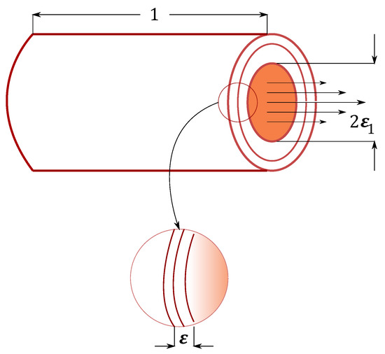
Figure 1.
A thin tube with radius , covered by an elastic wall of thickness .
Note that, although the main application of this model is related to hemodynamics, it can be applied to viscous flows in industrial installations, for example, for the thin tube structures in [].
2. Formulation of the Three-Dimensional Problem and Its Asymptotic One-Dimensional Approximation
Let us recall the formulation of the problem and the main result of [].
Consider a fluid occupying the interior of a thin cylindrical elastic tube (as shown in Figure 1) with the radius denoted by . More precisely, ref. [] studies a periodic direction problem in longitudinal space, where is defined as the ratio between the radius of the fluid domain and the length of the period, taken to be equal to one. The second small parameter is the elastic tube thickness with
The fluid and the elastic parts of the domain are defined, respectively, by
Supposing that the coupled problem is axisymmetric and denoting , let us associate the following layers in the plane to and :
The boundaries of the fluid and elastic layers and are denoted by
with the second one representing the interface surface.
The characteristics of the elastic medium are represented by the variable density depending on the radial variable, and by the matrix-valued coefficients , which depend on the Young’s modulus and on the Poisson’s ratio , with , . Because the density and the Young’s modulus characterizing a solid phase may be very different (high contrast) from one material to the other, it is interesting to analyze the changes in the mathematical model with respect to these physical characteristics. For this purpose, we introduce two additional parameters related to :
The density of the elastic tube is supposed to be of order and its Young’s modulus to be of order , while the characteristic time, the dynamic viscosity and the density of the fluid are supposed to be scaled so that they are of order one. So, and , with and E of order one. With respect to the physical characteristics of the elastic medium, we consider the following assumptions imposed for physical reasons:
With respect to the magnitude of , the following different cases are identified:
- (1)
- (2)
- (3)
- (4)
- (5)
In most practical applications, the relation between the density of an elastic medium and its Young’s modulus is . However, in order to simplify the illustration, we start with the relation
and then we pass to the case
and we present the results if there are major differences with respect to the case (7).
Some practical examples from biology and engineering are given in the introductory part of [].
Let us now give the formulation of the problem. Consider the stiffness matrices having the elements , which satisfy the relations
with the properties:
- (i)
- ,
- (ii)
- independent of such that , with .
The functions are supposed to be piecewise-smooth, and satisfies the following condition:
So, the wall can be a natural laminate, as is the case with blood vessels. The characteristics of the viscous fluid, independent of , are the positive constants and representing its density and its dynamic viscosity, respectively. They are supposed to be of order one.
In addition to the data (for the elastic medium) and (for the viscous fluid), we also consider as data of the problem the forces g and f, which represent an external action on the elastic medium and on the fluid, respectively. In the case of blood vessels, it corresponds to the action of the surrounding tissues; see [].
The mathematical model of the periodic, axisymmetric, time-dependent interaction between an incompressible, Stokes fluid and a cylindrical, stratified, elastic tube uses the following notation and expressions for: the linear elasticity operator, the divergence operator (for a vector-valued function and a symmetric tensor-valued function), the gradient operator (for a vector-valued function) and the velocity strain tensor with respect to the cylindrical coordinates:
Here are the cylindrical coordinates; and are the unit vectors of and axes, respectively; represents a vectorial function; S represents a tensorial axisymmetric function; and In a two-dimensional setting, taking into account only the “” and “r” components, we will use the notation
The mathematical model describing the fluid–elastic structure interaction in a thin-walled elastic tube with periodicity condition along the tube and homogeneous initial conditions is given by
The positive constant T appearing in this system gives the time interval of the problem, and it can be arbitrarily chosen, independently of .
The main result of [] is the construction of a complete asymptotic expansion of the solution in all the cases cited above, the evaluation of the norms of the error for the truncated expansions, and the computation of the leading term of the expansion, which is some analogue of the Poiseuille flow for tubes with elastic walls. Classical Poiseuille flow is defined as a flow with a given pressure drop at the ends of a tube. Formally, the problem (11) does not include such a case, because of the periodicity condition along the tube. However, such a pressure drop can be created in half of a tube. Then, the leading term of the asymptotic expansion of the solution, independently of the considered cases, can be interpreted as a Poiseuille-type flow; the velocity of the fluid and the displacements in the walls are expressed via three basic functions depending on the normal variable and time only. One of them is the scaled average velocity Q (the averaged velocity is equal to ), the second is the longitudinal displacement of the wall-fluid interface , and the third is the leading term for the pressure, q:
Here, for the leading terms, we keep the same notation as for the exact solution.
Note that the leading term for pressure, q, is related to the scaled average velocity Q by
so that there are only two independent basic functions of the leading term of the ansatz, and the radial displacement of the wall-fluid interface, , can be approximately calculated as
and so,
If we need a continuous approximation of the velocity at the interface, then we have to add the third order terms in the approximation of :
Note that the classical notion of the Poiseuille flow in an axisymmetric thin cylinder corresponds to the parabolic shape of the normal velocity of the flow and vanishing radial velocity. It was first described by J.L.M. Poiseuille and J. Boussinesq [,], and it takes place only for the stationary Stokes or Navier–Stokes equations. In the time-dependent case with no slip condition at the boundary (absolutely rigid wall), its analogue is the so-called Womersley flow [,], when the normal velocity is just independent of the normal coordinate, and the radial velocity still vanishes. However, in the case of a flow in a tube with an elastic wall, the normal velocity depends on the normal coordinate because the cross-section changes over time. Therefore, a Poiseuille-type flow is quite different from a flow with a rigid wall. The first term in formula (12) is the “trace” of the rigid wall case. If the longitudinal velocity of the wall vanishes, then this term coincides with the result of []; the relation (13) coincides with the earlier known relations for the pressure slope and the average velocity (Darcy law), and the relations for the cross-section area and the average velocity (mass conservation law).
Relations (12) and (13) with two free basic functions Q and can be used as an ansatz in the frame of the method of asymptotic partial decomposition of the domain for the fully three-dimensional problem for the Stokes or Navier–Stokes equations in a network of vessels with fluid–structure interaction at the interface with elastic walls. Namely, the weak formulation of the full problem can be restricted to a subspace of functions having the form (12) and (13) within all cylindrical parts of a network at some distance from the bifurcations, similarly to the approach proposed in simpler cases in [,]. For the Navier–Stokes equations, formal analysis shows that the same ansatz can be used, but relation (13) should be modified in order to take into account non-linear terms. This approach allows us to reduce the number of dimensions to one in all cylindrical parts of the network and reduces the computational costs and computer memory required.
Comparing the ansatz (12) to the one-dimensional model [], one can check that the leading term of the velocity satisfies the first equation of the system of equations
where is the area of the cross-section at the point , and is the flux at the same point. However, the second equation of [] differs from the equation below. This is explained by a different approach to the derivation of the one-dimensional model and the absence of the convective term in the formulation of the fluid–structure interaction problem.
Note that in models [,,], the first equation of the system is the same.
3. The Variational Framework of the Problem
The first part of this section is devoted to the presentation of the functional spaces we are dealing with. Because our functions are periodic with respect to , we introduce the periodicity domains for the fluid and for the elastic tube, respectively:
and the corresponding periodicity plane domains
The boundaries corresponding to and are denoted by
Let us introduce the following weighted spaces for the fluid part of the domain:
where
For periodic in functions, we introduce the periodic weighted spaces: is the space of functions defined on , periodic in , with the restriction to any arbitrary rectangle in and , where . The space of the traces of functions from is denoted by and, if we are interested only of the properties on a subset , we shall write , for l integer, . The space represents the dual of the subspace of containing functions that vanish on .
For the elastic part of the domain, the classical Sobolev spaces are used: , see [,], (as in we have , ). Additionally, we introduce the periodic spaces , defined in a similar way as for the fluid domain and the classical trace spaces. However, we write , etc., to show that the integrands in the norm contain the factor r.
The spaces that contain some of the properties given by (11) for the displacement and for the velocity, as well as the expected regularity of these functions, are defined by
In order to present the space containing the coupling condition, let us set for any defined on and belonging to a certain functional space H,
and then
Note that the space H should have enough regularity to give sense to the trace of on .
Remark 1.
In the axisymmetric problem, associate to any arbitrary function the function such that
with . The function Ψ is expressed with respect to the Cartesian coordinates and unit vectors and standard calculations give if and only if , .
In [], it is assumed that
In the framework presented above, the variational formulation of system (11), studied in [], is given by
where , defined by
is the bilinear form associated with the elasticity operator L. The results concerning the existence, the uniqueness and the regularity of the unknown functions are obtained in [].
4. Modified Variational Formulation for the Numerical Setup
We will modify the boundary conditions at the ends of the tube. Instead of the periodic solution with respect to the variable , we introduce some given inflow and outflow, supposing that the elastic tube is clamped at the ends of the tube. Namely, the periodic boundary conditions (11) are replaced by a given velocity for and for , and by vanishing displacements u = 0 for x3 = 0 and x3 = 1. Here gin and gout are given differentiable functions vanishing at t = 0. On the right-hand side, g and f are taken to be equal to zero. So, the problem is
Respectively, the variational formulation is changed. Let us define the spaces
and
Multiplying (28) by functions of the base in with some coefficients , and summing up and varying , we obtain the equivalent integral equation.
Here, is the average velocity, and is the flux.
Equation (29) can be rewritten in the following form:
Finally, we consider a projection of this variational formulation to the “ansatz space” of test functions having the form (12) with q given by (13), with arbitrary free basic functions Q and from . The solution is sought in the closure with respect to the norm of the space of functions having the form (12) with smooth base functions.
In the following, we consider a simplified ansatz, assuming that and taking only a part of the terms in (12). This assumption is often satisfied in the blood vessels, such that the vessel does not move very much in the direction of blood flow. Namely, we consider the following space of test functions:
where vanishes with its first derivatives in for and , and vanishes with its first derivatives in t for and . Furthermore, we will replace the notation of the basic function Q for the space of test functions with R. Additionally, we assume that functions and satisfy the conditions and , where , and we seek a solution with Q satisfying the relations . The test functions are also considered, with R satisfying the same relations: .
Next, we will consider a shorter approximation for the solution:
We assume that and are constants; therefore, from (33), we have the following expressions:
As the boundary conditions for the solution, we use the value of equal to the average velocity at the inlet and outlet, and the derivative is equal to zero.
Substituting (34) into the following integral identity:
we obtain the fourth order differential equation describing the elastic wall Poiseuille equation (EWPE):
where
5. Numerical Scheme for the Poiseuille Equation
In this section, we numerically solve the following boundary value problem for the elastic wall Poiseuille equation (EWPE) (36):
We introduce uniform meshes of points in space and time with step sizes equal to h and , respectively:
Then, the numerical solution to (37) at grid point is denoted by .
The derivatives of even order in (37) are discretized using central differences, while the derivatives of the first order are discretized using forward differences. The resulting scheme is implicit. Applied at each inner point of the spatial mesh, it forms a tridiagonal matrix problem, which is effectively solved using the Thomas algorithm.
Using the standard method of Taylor expansions, it is easy to check that, with sufficient smoothness conditions, the order of accuracy of this scheme is . Note that a central-difference discretization of the first-order derivatives would result in higher accuracy in time; however, the stability of such a scheme would be hardly attainable in practical computations, where the parabolic terms of (37) are dominant.
Using the classical stability analysis, it is easy to show that, for the practical problems that we are interested in, the numerical stability Courant–Friedrichs–Lewy (CFL) condition holds, with some constant c that depends on the parameters of the model.
We seek the scaled average velocity Q in m/s inside a small elastic tube or capillary with the Young modulus Pa, the Poisson ratio , the length of the tube m, the radius m, the thickness m and the dynamic viscosity of blood Pa·s. The following set of constants is obtained:
To test the accuracy of the constructed solver, let us define the error in the maximum norm by e, and the experimental convergence rates in space and time by and :
Here, is a benchmark solution, which is computed using very small step sizes.
The results of experimental convergence tests are presented in Table 1 below. Here, the functions , were used, and the problem was solved for . We can see from the results of Table 1 that the experimental convergence rate agrees well with the theoretical estimate.

Table 1.
Errors and experimental convergence rates for sequences of step sizes in space (left) and time (right). The results confirm experimentally that the order of accuracy of the numerical scheme is .
6. Numerical Comparison of the Approximate 1D Model and the Full-Dimensional Problem
In the present section, we compare the numerical solutions of two problems: the full-dimensional Navier–Stokes equations with the fluid–structure interaction (FSI) conditions for the tubes with an elastic wall, and the EWPE approximation.
- Solution in a single vessel
We consider two types of inflow/outflow boundary conditions: first, ; second, with ; and compare the solutions in the middle point of the tube (Figure 2 and Figure 3).
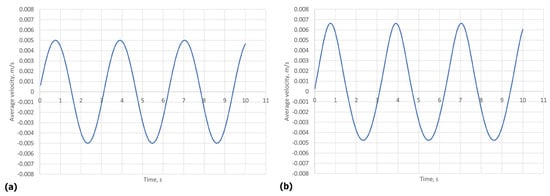
Figure 2.
(a) presents the average velocity computed by EWPE (the fourth order PDE (37)) over time, (b) depicts the average solution (velocity) of the full Navier–Stokes model. In both cases, , and the solution was taken from the middle cross-section of the tube.

Figure 3.
(a) presents the average velocity according to the EWPE approximation over time, (b) depicts the average velocity of the full Navier–Stokes model. In both cases, , and the solution was taken from the middle cross-section of the tube. Note that here we deliberately simulate a case of large displacement of the wall, in order to explore the limitations of the ansatz.
For and , the difference between the solutions is less than 10 per cent. When increases (, ), the difference is more significant. This can be explained by important variations of the cross-section (more than two times). In this case, the assumption of small displacements of the wall is no more realistic, and so the model must take into consideration the difference between Eulerian and Lagrangian approaches.
- Solution in a Y-shaped network of vessels
Next, we compare the solutions acquired from (37) and the full Navier–Stokes in a Y-shaped network (see Figure 4), where the inflow is on the left and two outflows are on the right. The corresponding boundary conditions are and for each of the two outlets to the right, while the Young modulus is Pa for the tube-shaped blood vessel wall and Pa for the sphere-shaped connection of three tubes, the Poisson ratio , the length of each of the three tubes m, the radius m, the wall thickness m, and the dynamic viscosity of blood Pa·s. The large Young’s modulus of the wall in the bifurcation zone simulates the no-slip boundary condition there. It corresponds to the experimental observation that, near the bifurcations, the vessels become much stiffer than the “tube” walls.
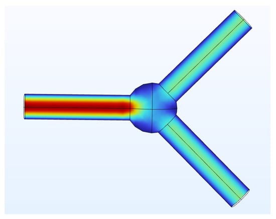
Figure 4.
Geometry of the Y-shaped bifurcation model.
The EWPE approximation uses the following junction conditions at the bifurcation node: (1) the flux coming from the left tube is equal to the sum of the fluxes going out into the left tubes (this condition corresponds to a stiffer bifurcation zone of vessels); (2) the first derivatives for all tubes at the bifurcation node; and (3) the second derivatives at the bifurcation node for the tubes on the right.
Figure 5 and Figure 6 display the graphs of average velocity in the midpoints of the left and right vessels, respectively, up to T = 10.
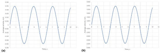
Figure 5.
(a) presents the average velocity given by the EWPE approximation (37) over time, (b) depicts the average velocity given by the full Navier–Stokes model. In both cases, , , and the solution was taken from the middle cross-section of the left tube.
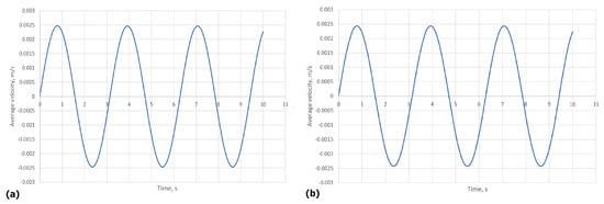
Figure 6.
(a) presents the average velocity given by the EWPE approximation (37) over time, (b) depicts the average velocity given by the full Navier–Stokes model. In both cases, , , and the solution was taken from the middle cross-section of either of the right tubes.
7. Conclusions
A 1D elastic wall quasi-Poiseuille approximation for the fluid–structure interaction problem in a cylindrical tube is introduced and tested numerically by comparison with the full-dimensional Navier–Stokes–elastic shell FSI problem. One-tube and tube network geometries are considered. The inflows and outflows with and without flux conservation are tested. The results show a good approximation for the fluid–structure interaction model in the case of small displacements of the wall and modest Reynolds numbers.
Author Contributions
Conceptualization: G.P.; Formal analysis: K.K., N.K., G.P., K.P., V.Š.; Software, numerical computations N.K., V.Š. All authors have read and agreed to the published version of the manuscript.
Funding
The work has received funding from the European Social Fund (project No 09.3.3-LMT-K-712-17-0003) under a grant agreement with the Research Council of Lithuania (LMTLT).
Conflicts of Interest
The authors declare no conflict of interest.
References
- Desjardins, B.; Esteban, M.J.; Grandmont, C.; le Talec, P. Weak solutions for a fluid-structure interaction model. Rev. Mat. Comput. 2001, 14, 523–538. [Google Scholar] [CrossRef]
- Gilbert, R.P.; Mikelić, A. Homogenizing the acoustic properties of the seabed: Part I. Nonlin. Anal. Theory Methods Appl. 2000, 40, 185–212. [Google Scholar] [CrossRef]
- Grandmont, C.; Maday, Y. Existence for an unsteady fluid-structure interaction problem. Math. Model. Numer. Anal. 2000, 34, 609–636. [Google Scholar] [CrossRef]
- Čanić, S.; Mikelić, A. Effective equations modeling the flow of a viscous incompressible fluid through a long elastic tube arising in the study of blood flowthrough small arteries. SIAM J. Appl. Dyn. Syst. 2003, 2, 431–463. [Google Scholar] [CrossRef]
- Čanić, S.; Tambača, J.; Guidoboni, G.; Mikelić, A.; Hartley, C.J.; Rosenstrauch, D. Modeling viscoelastic behavior of arterial walls and their interaction with pulsate blood flow. SIAM J. Appl. Math. 2006, 67, 164–193. [Google Scholar] [CrossRef]
- Mikelić, A.; Guidoboni, G.; Čanić, S. Fluid-structure interaction in a pre-stressed tube with thick elastic walls. I. The stationary Stokes problem. Netw. Heterog. Media 2007, 2, 397–423. [Google Scholar] [CrossRef]
- Panasenko, G.P.; Stavre, R. Asymptotic analysis of a periodic flow in a thin channel with visco-elastic wall. J. Math. Pures Appl. 2006, 85, 558–579. [Google Scholar] [CrossRef]
- Panasenko, G.P.; Sirakov, Y.; Stavre, R. Asymptotic and numerical modeling of a flow in a thin channel with visco-elastic wall. Int. J. Multiscale Comput. Eng. 2007, 5, 473–482. [Google Scholar]
- Panasenko, G.P.; Stavre, R. Asymptotic analysis of a non-periodic flow with variable viscosity in a thin elastic channel. Netw. Heterog. Media 2010, 5, 783–812. [Google Scholar] [CrossRef]
- Malakhova-Ziablova, I.; Panasenko, G.; Stavre, R. Asymptotic analysis of a thin rigid stratified elastic plate—Viscous fluid interaction problem. Appl. Anal. 2016, 95, 1467–1506. [Google Scholar] [CrossRef]
- Panasenko, G.P.; Stavre, R. Viscous fluid-thin elastic plate interaction: Asymptotic analysis with respect to the rigidity and density of the plate. Appl. Math. Optimiz. 2020, 81, 141–194. [Google Scholar] [CrossRef]
- Panasenko, G.P.; Stavre, R. Viscous fluid-thin cylindrical elastic body interaction: Asymptotic analysis on contrasting properties. Appl. Anal. 2019, 98, 162–216. [Google Scholar] [CrossRef]
- Panasenko, G.P.; Stavre, R. Three dimensional asymptotic analysis of an axisymmetric flow in a thin tube with thin stiff elastic wall. J. Math. Fluid Mech. 2020, 22, 35. [Google Scholar] [CrossRef]
- Formaggia, L.; Lamponi, D.; Quarteroni, A. One-dimensional models for blood flow in arteries. J. Eng. Math. 2003, 47, 251–276. [Google Scholar] [CrossRef]
- Gamilov, T.M. Mathematical Modeling of Blood Flow under Mechanical Action at Vessels. Ph.D. Thesis, Moscow Physics and Technology Institute, Moscow, Russia, 2017. [Google Scholar]
- Koshelev, V.B.; Mukhin, S.I.; Sosnin, N.V.; Favorsky, A.P. Mathematical Models for Quasi-One-Dimensional Hemodynamics; MAKS Press: Moscow, Russia, 2010. [Google Scholar]
- Simakov, S.S.; Kholodov, A.S.; Evdokimova, A.V. Methods for computing global blood flow in the human’s body by heterogeneous numerical models. In Medicine in the Mirror of Informatics; Nauka: Moscow, Russia, 2008; pp. 124–170. [Google Scholar]
- Long, G.; Liu, Y.; Xu, W.; Zhou, P.; Zhou, J.; Xu, G.; Xiao, B. Analysis of crack problems in multilayered elastic medium by a consequtive stiffness method. Mathematics 2022, 10, 4403. [Google Scholar] [CrossRef]
- Boussinesq, J. Essaii sur la Théorie des Eaux Courrantes. In Mémoires Présentés par Divers Savants de l’Académie des Sciences de l’Institut de France; Impr. Nationale: Paris, France, 1877. [Google Scholar]
- Poiseuille, J.L.M. Recherches sur les Causes du Mouvement du Sang dans les Vaisseaux Capillaires; Impr. Royale: Paris, France, 1839. [Google Scholar]
- Galdi, G.P.; Pileckas, K.; Silvestre, A.L. On the unsteady Poiseuille flow in a pipe. Z. Angew. Math. Phys. 2007, 58, 994–1007. [Google Scholar] [CrossRef]
- Womersley, J.R. Method of calculation of velocity, rate of the flow and viscous drag in arteries when the pressure gradient is known. J. Physiol. 1955, 127, 553–563. [Google Scholar] [CrossRef] [PubMed]
- Berntsson, F.; Ghosh, A.; Kozlov, V.A.; Nazarov, S.A. A one-dimensional model of blood flow through a curvilinear artery. Appl. Math. Model. 2018, 63, 633–643. [Google Scholar] [CrossRef]
- Panasenko, G.P.; Stavre, R. Asymptotic analysis of a viscous fluid-thin plate interaction: Periodic flow. Math. Mod. Meth. Appl. Sci. 2014, 24, 1781–1822. [Google Scholar] [CrossRef]
- Evans, L.C. Partial Differential Equations. In Graduate Studies in Mathematics, 2nd ed.; American Mathematical Society: Providence, Rhode Island, 2010; Volume 19. [Google Scholar]
- Temam, R. Navier-Stokes Equations; North-Holland Publishing Company: Amsterdam, The Netherlands; New York, NY, USA, 1977. [Google Scholar]
Disclaimer/Publisher’s Note: The statements, opinions and data contained in all publications are solely those of the individual author(s) and contributor(s) and not of MDPI and/or the editor(s). MDPI and/or the editor(s) disclaim responsibility for any injury to people or property resulting from any ideas, methods, instructions or products referred to in the content. |
© 2023 by the authors. Licensee MDPI, Basel, Switzerland. This article is an open access article distributed under the terms and conditions of the Creative Commons Attribution (CC BY) license (https://creativecommons.org/licenses/by/4.0/).