Abstract
One important parameter in the Black–Scholes option pricing model is the implied volatility. Implied volatility surface (IVS) is an important concept in finance that describes the variation of implied volatility across option strike price and time to maturity. Over the last few decades, economists and financialists have long tried to exploit the predictability in the IVS using various parametric models, which require deep understanding of financial practices in the area. In this paper, we explore how a data-driven machine learning method, symbolic regression, performs in identifying the implied volatility surface even without deep financial knowledge. Two different approaches of symbolic regression are explored through a simulation study and an empirical study using a large panel of option data in the United States options market.
Keywords:
implied volatility surface; symbolic regression; recurrent neural network; genetic programming MSC:
68U99
1. Introduction
Accurate pricing models are crucial for trading, hedging, and managing risk in option portfolios. In 1973, Black, Scholes, and Merton introduced their famous option pricing model, which is now known as the Black–Scholes (BS) model. This model assumes that the underlying stock follows a Brownian motion with a constant drift and volatility. Despite its simplicity, the Black–Scholes model and its variants remain the most widely used option pricing models in finance today.
One critical parameter in the Black–Scholes option pricing model is market volatility, which can be estimated using implied volatility. To calculate implied volatility, one inputs the market price of the option into the Black–Scholes formula and back-solves for the value of the volatility. Implied volatility is an estimate of the asset’s future variability that underlies the option contract. In the Black–Scholes framework, volatility is assumed to be constant across strikes, time to maturity, and time. However, in reality, there are variations in implied volatility across option strikes and time to maturity. Canina and Figlewski [1] demonstrated that when plotting implied volatility against moneyness (the ratio between the strike price and underlying spot price) for a given time to maturity, the resulting plot often resembles a smile or skew in shape. This variation in implied volatility across different time to maturity and moneyness is known as the implied volatility smile. An implied volatility surface (IVS, for the remaining of the paper, IVS only refers to the implied volatility surface) is a 3D plot that plots implied volatility smile and term structure of volatility in a three-dimensional surface for all options on a given underlying asset.
In recent decades, economists and finance experts have sought to exploit the predictability of the IVS. Dumas, Fleming, and Whaley [2] proposed a linear model of implied volatility over strike price and time to maturity. However, when they applied the model to a weekly cross-section of S&P 500 options prices, they found that coefficient estimates were highly unstable. In 2000, Heston and Nandi [3] developed a moving window non-linear GARCH(1,1) model for the IVS. While their approach was an improvement over previous methods, they also found that some of the coefficients were unstable. Goncalves and Guidolin [4] proposed a method that models the implied volatility over a time-adjusted measure of moneyness and time to maturity. This method represents the culmination of several decades of research into the predictability of the IVS and requires a deep understanding of financial practices in this area.
What if we lack thorough knowledge of the area? Can we use data-driven methods instead of human intelligence to identify a reasonable functional form for IVS? Additionally, is it possible to use data-driven methods to determine useful features that impact the IVS? Traditional machine learning models such as random forest, gradient boosting, etc., can provide desirable prediction performances. However, the models proposed by these methods are non-parametric and cannot have any interpretation in finance. Moreover, these models can be highly sensitive to the tuning of hyperparameters.
Symbolic regression is a machine learning approach that can discover the underlying mathematical expressions describing a dataset, which could be a viable method for studying the actual relationship between IVS, moneyness, and time to maturity. The advantage of symbolic regression is that it can identify the relationship between input variables and output variables in a given dataset without a predefined functional form. In recent years, this method has been used in areas such as physics and artificial intelligence (AI). The most commonly used approach for symbolic regression is genetic programming (GP), which was proposed and improved by Schmidt and Lipson [5] and Back et al. [6]. Udrescu and Tegmark [7] proposed a physics-inspired method for symbolic regression called AI Feynman, which has proven successful in discovering all 100 equations from the Feynman Lectures on Physics. Peterson et al. [8] presented the approach called deep symbolic regression (DSR), which is a gradient-based approach for symbolic regression. One commonality among these methods is that they have only been used and tested on data with low noise levels.
In this paper, we aim to explore whether symbolic regression approaches can have good performance in discovering mathematical relationships among IVS, moneyness, and time to maturity using financial data with high noise levels. We also adopt Bayesian optimization to tune hyperparameters for symbolic regression.
This paper is structured as follows. Section 2 provides a brief introduction to implied volatility surface (IVS). Two symbolic regression approaches, GP and DSR, are introduced in detail in Section 3. In Section 4, we thoroughly introduce the parameter tuning approach, Bayesian optimization. Simulation studies are conducted in Section 5, and a real data analysis is presented in Section 6. Finally, in Section 7, we summarize the paper.
2. Implied Volatility Surface
Before diving into the concept of Implied Volatility Surface, it is important to understand the Black–Scholes (BS) model. The BS model is an option pricing model widely used by market participants such as hedge funds to determine the theoretically fair value of an option contract. The model was first proposed by Black, Scholes and Merton in 1973. The Black–Scholes model can only be used to calculate the price of a European option. A European option is a version of an option contract that limits execution to its expiration date. It allows the holder to potentially transact on an underlying asset at a preset price. There are two types of European options: the call option and the put option. A European call option gives the owner the right to acquire the underlying asset at the expiration date for the preset price, while a European put option allows the holder to sell the underlying asset at expiry for the preset price. These pre-specified prices are called strike prices.
The BS model assumes the price of the underlying asset, which follows a geometric Brownian motion with constant drift and volatility, that is:
where is the price of the asset at time t, is the drift, is the volatility, and is the standard Brownian motion. Black and Scholes [9] proposed a partial differential equation (PDE) governing the price evolution of a European option under the Black–Scholes model. The Black–Scholes formula is a solution to the Black–Scholes PDE, which calculates the price of European put or call options. Without loss of generality, let us suppose we have a call option with price C, then
where K is the strike price, which is the fixed price for the asset that can be bought by the option holder; T is time to maturity, which represents the time until the option’s expiration; is the current price of the underlying asset, r is the risk-free interest rate, and is the cumulative standard normal distribution function. is the constant volatility. We can solve for the unknown volatility through Equation (2) using the observed option prices to obtain the implied volatility (IV).
If the assumptions in the Black–Scholes model hold, for options written on the same underlying but with different strike price or time to maturity, the implied volatility would be the same. However, this is not observed in practice.
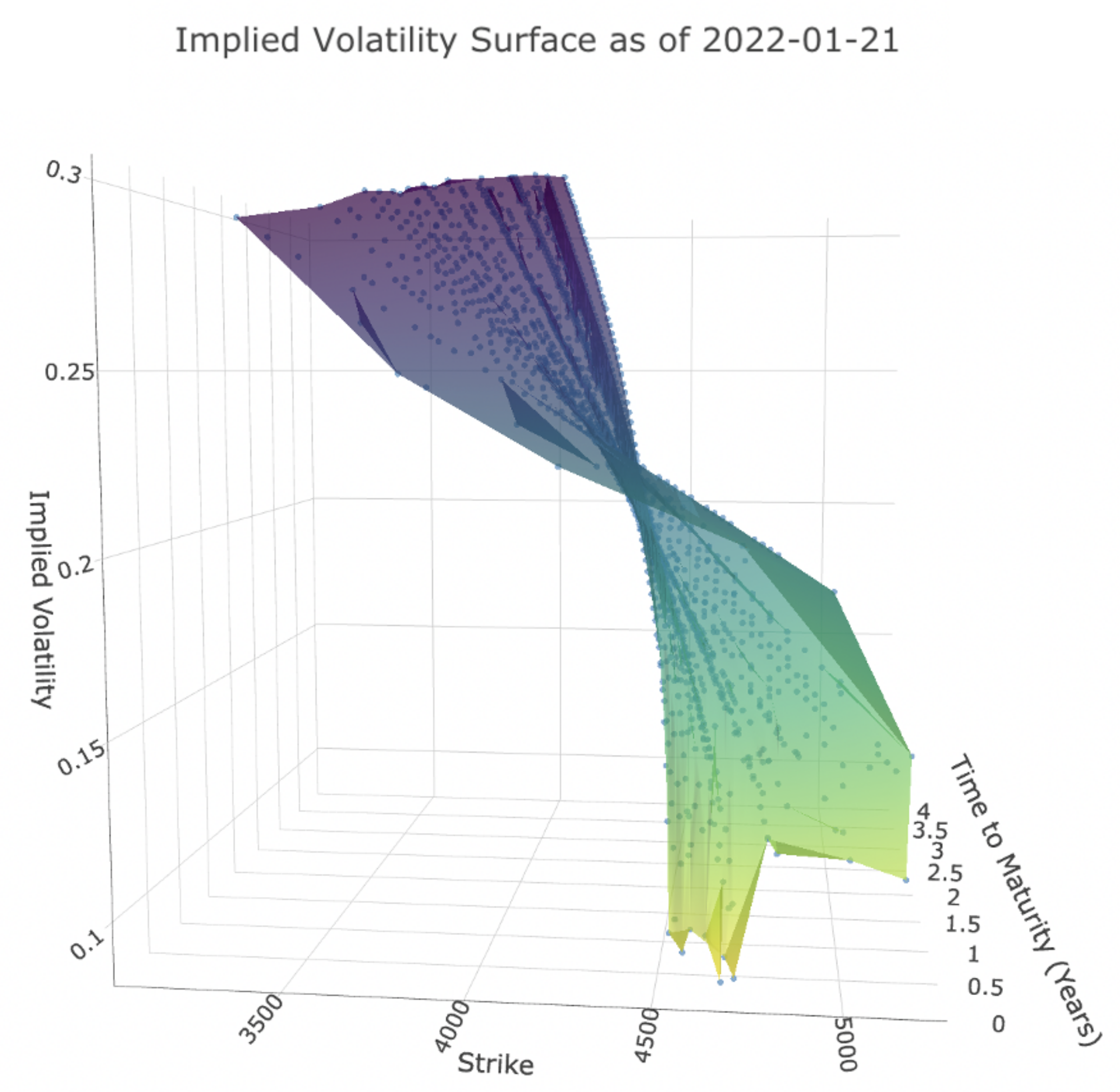
Figure 1 shows the volatility surface for put options from 30 stocks from the S&P 500 Index on 21 January 2022. These data will also be used in our empirical study. It is apparent that lower strikes tend to have higher implied volatility. Additionally, for a given time to maturity T, the curve of implied volatility and strike exhibits a skew or smile shape. The observed changes in implied volatility with strike and maturity contradict the Black–Scholes assumption. Therefore, the objective of this paper is to estimate this surface as a function of all K and T, that is, find a functional form of where t indicates its time-dependence.

Figure 1.
Implied volatility surface for put options from S&P 500 Index on 21 January 2022.
Several economists have dedicated years of effort to understand this empirical scenario using financial theories and building models to predict IVS. In this paper, we attempt to explore the ability of a machine learning (ML) method called symbolic regression to identify IVS using moneyness (a term that describes the relationship between the strike price of an option and the underlying price of the asset) and time to maturity, without requiring an in-depth understanding of financial theories.
3. Symbolic Regression
Symbolic regression is a type of analysis that performs function identification. The goal of symbolic regression is to identify the relationship between input variables and output variables in a given dataset and to express this relationship in mathematical equations. Unlike other methods, symbolic regression does not require a predefined functional form and aims to generate a model. Symbolic regression is typically based on evolutionary computing (EC) techniques and is widely used. However, non-EC methods for symbolic regression have also been discussed recently. In Section 3.1, we will introduce symbolic regression using genetic programming, which is an EC method. In Section 3.2, we will discuss a non-EC approach called deep symbolic regression.
3.1. Symbolic Regression via Genetic Programming (GP-SR)
3.1.1. Genetic Programming
Genetic programming (GP) was first proposed in Koza et al. [10]. It is an evolutionary computation method that can automatically address problems without requiring a pre-specified structure. GP begins with a population of randomly generated programs, which evolve generation by generation to obtain better fitness. During this process, the fittest programs are expected to be found. GP has been widely applied to symbolic regression problems, and in this subsection, we will introduce how GP can be used for symbolic regression in more detail.
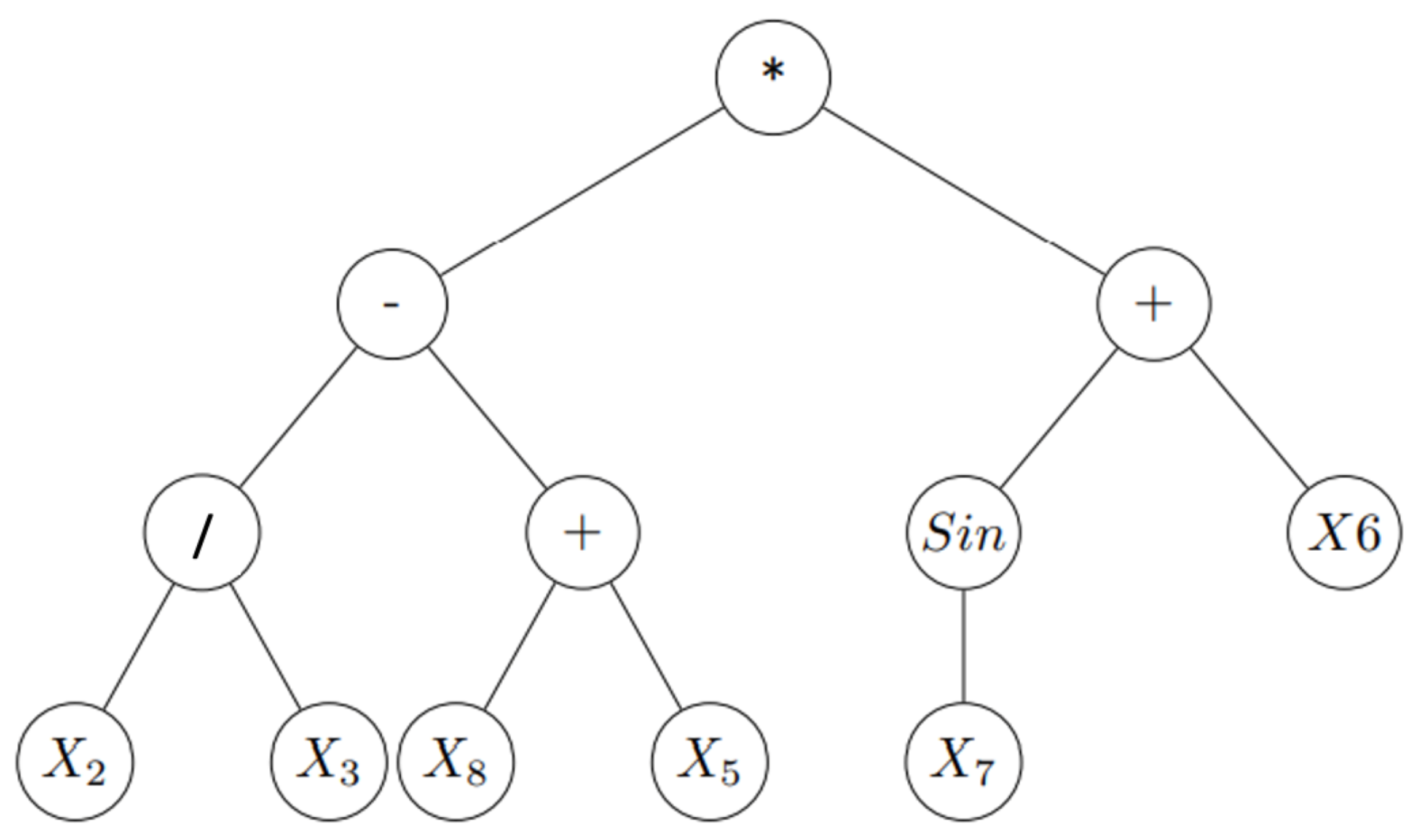
When using genetic programming in symbolic regression (GP-SR), programs are mathematical formulas that can be represented using sparse trees. Figure 2 shows the tree that represents .
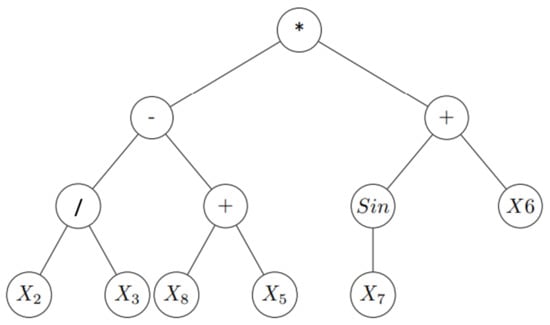
Figure 2.
GP tree for -. Nodes contain functions (add, minus, etc.), variables (, , etc.) and constants, and nodes with variables and constants are called terminal nodes. We usually read these trees starting with the left-hand leaves.
In order to generate populations of formulas, function set F (addition, subtraction, multiplication, etc.) and terminal set E (constants, parameters, etc.) should be pre-prepared. In the above example, ×, −, +, and/are in the function set F, and ’s are in the terminal set E. Each element in the function set F has a fixed number of arguments. For example, + has two arguments and has one argument.
3.1.2. Initialization
The first step in GP-SR is generating the initial population of formulas with size n; here, n is pre-specified. There are three ways to generate the initial population: grow, full and half and half.
Grow is the simplest one where nodes are chosen at random from function set F and terminal set E before the maximum tree size or limited tree depth is reached. This method tends to select smaller formulas than the max depth we specified, since terminals can be chosen before max depth is reached.
Full method, on the contrary, only produces tress with a full size. The method chooses nodes from the function set until the max depth is reached, and then, terminals are chosen.
The final method half and half is the combination of the previous two methods. That is, in this method, half of the formulas in the initial population are generated with the full method, and the other half are produced by the grow method. This method produces a mixture of formula tree shapes and depths.
In the first step of the GP-SR, using one of the above methods, we generated the initial population that contains the number of formulas equal to the population size n pre-specified.
3.1.3. Selection
Now that we have our initial population of formulas, we need to decide the ones that will evolve into the next generation. First, we need to measure the performances of each formula on the training data using common error metrics such as mean absolute error () and root mean square error (). After the performances of individual formulas have been evaluated, better fitted formulas need to have more opportunities to evolve into the next generation. Based on this idea, GP-SR utilizes a selection method called the tournament selection.
In the tournament selection, a smaller subset of formulas are selected at random from the population in the current generation. The number of formulas chosen is determined by the tournament size, which is pre-specified. These formulas are compared with each other and the one that fits the data the best will be selected to move on to the next generation as a parent. If the tournament size is large, we might find fitter formulas more quickly. A smaller tournament size will maintain more diversity in the population and may find a better solution at longer time.
3.1.4. Genetic Operations
After we choose a parent from the current generation, evolution proceeds by transforming parents to offspring using genetic operators. There are four commonly used genetic operators, crossover, subtree mutation, Hoist Mutation, point mutation and reproduction.
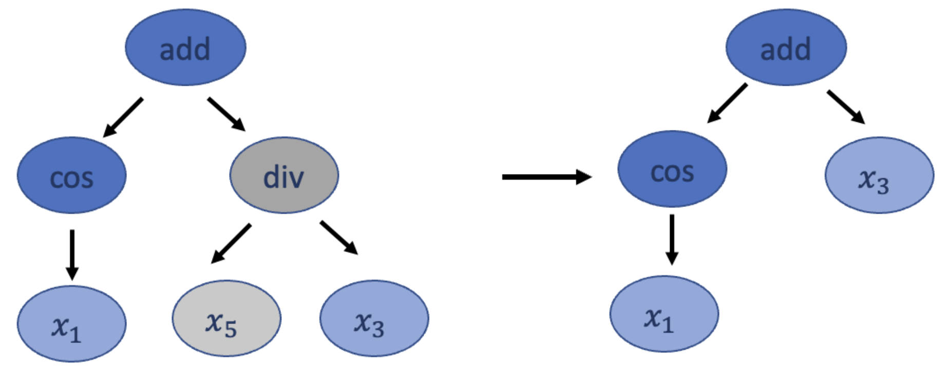
Unlike other genetic operations, the crossover requires two tournaments. In the first tournament, the winner is selected as the parent, and a random subtree is selected from it to be replaced. Then, another tournament is conducted and another winner is chosen to be a donor, and then, a random subtree is selected from the donor and is inserted into the original parent to form an offspring for the next generation. Figure 3 shows an example of the crossover transformation.

Figure 3.
An example for crossover. Gray nodes represent subtrees that need to be replaced. Blue nodes represent subtrees that are combined into a new tree to the next generation, while dark blue nodes contain functions and light blues nodes represent terminal nodes.
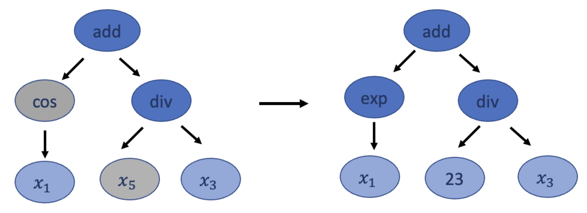
The subtree mutation takes a winner of the tournament as the parent and selects a random subtree from it to be replaced. At this time, the donor subtree will be generated randomly from the population and will be inserted to the parent to form an offspring for the next generation. Subtree mutation is very aggressive since subtrees from winners can be replaced by randomly generated components, but this can maintain the diversity in the population. Figure 4 shows an example of the subtree mutation transformation.

Figure 4.
An example of subtree mutation. Gray nodes represent the subtree that needs to be replaced. Blue nodes represent subtrees that are combined into a new tree to the next generation, while dark blue nodes contain functions and light blues nodes represent terminal nodes.
The hoist mutation takes a winner of the tournament as the parent and selects a random subtree from it. Then, a random subtree of that subtree is selected and is re-inserted into the original subtree’s location to form an offspring for the next generation. This mutation simply removes some genetic material from the winners. Figure 5 shows an example of the hoist mutation transformation.
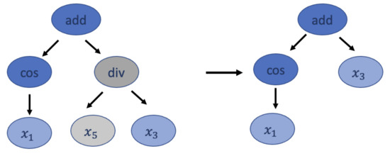
Figure 5.
An example for hoist mutation. Gray nodes represent the subtree that is removed from the parent. Blue nodes are nodes that remain, while dark blue nodes contain functions, and light blues nodes represent terminal nodes.
The point mutation takes a winner of the tournament as the parent and randomly selects nodes from it to be replaced. Functions are replaced by other functions, and terminals are replaced by other terminals with the same number of arguments. For example, function + can only be replaced by functions such as − and × since they all have two arguments. The resulting tree forms an offspring for the next generation. This method can also maintain the diversity in the population. Figure 6 shows an example of the point mutation transformation.
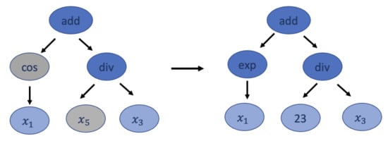
Figure 6.
An example for point mutation. Gray nodes represent nodes that have been replaced. Blue nodes are nodes that remain the same, while dark blue nodes contain functions, and light blues nodes represent terminal nodes.
The reproduction operator is straightforward. It clones the tournament winner and enters the next generation.
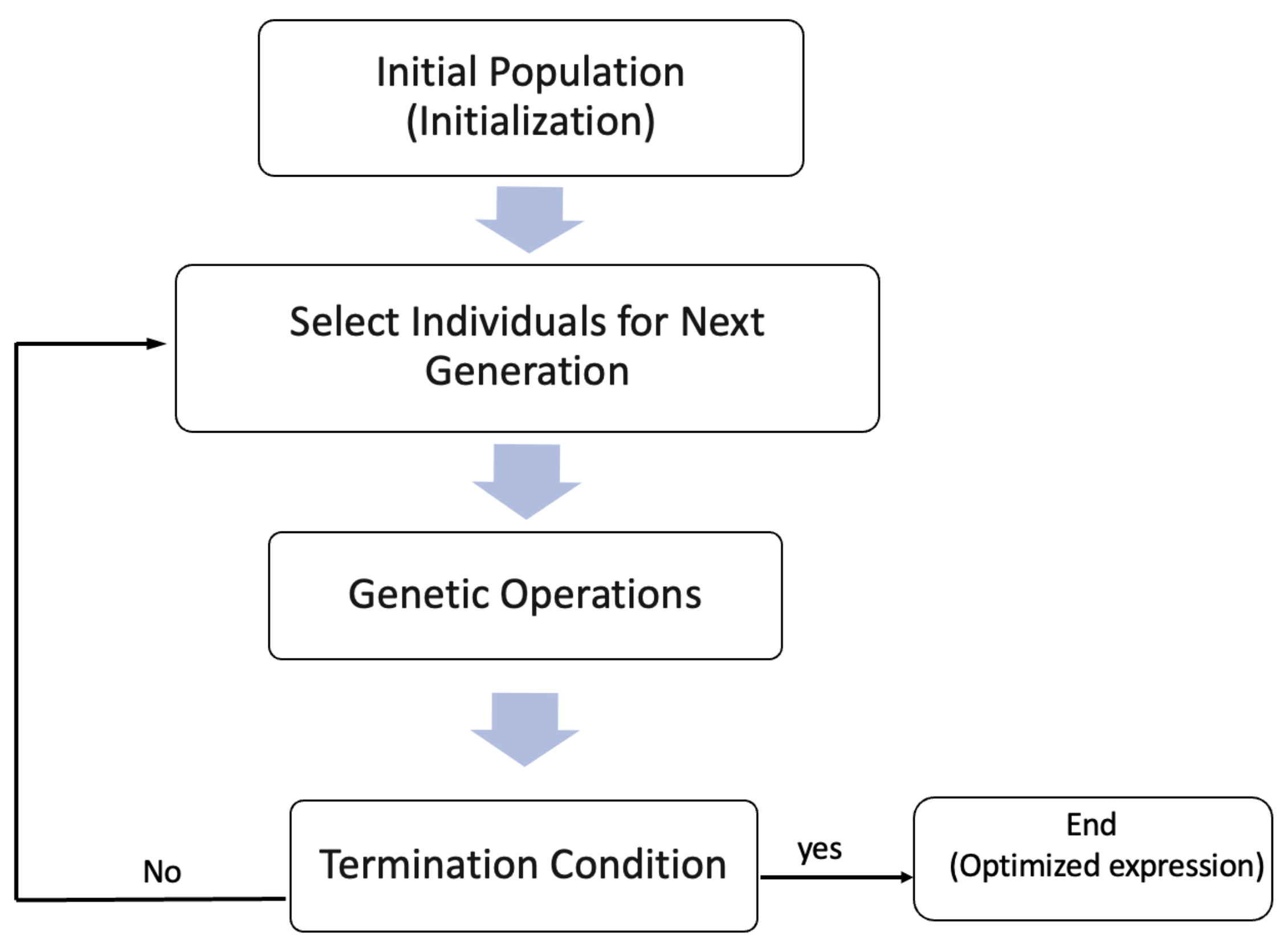
These operators will be utilized by the probabilities we specified in advance. The evolution procedure will stop if at least one formula in the evolution has the fitness reaching the threshold we pre-specified or the evolution has reached the maximum number of generations we pre-specified. The whole procedure is illustrated in the flowchart in Figure 7 below:

Figure 7.
The flowchart illustrates the procedure of the GP-SR.
3.2. Deep Symbolic Regression
Deep symbolic regression (DSR) is a novel symbolic regression approach proposed in Peterson et al. [8]. This method employs a unique approach used to identify the underlying mathematical formulas that describe a given dataset. Unlike GP-SR, DSR utilizes a large model to explore the space of small models. The fundamental idea behind DSR is to use a recurrent neural network (RNN) to generate a distribution over mathematical formulas and then to use a risk-seeking policy gradient to train the network and to generate better-fitted formulas.
3.2.1. Generating Expressions Using Recurrent Neural Network
An RNN is a type of artificial neural network that is designed to handle sequential data. In traditional neural networks, it is generally assumed that inputs and outputs are independent. However, this assumption may not hold true in some cases. For instance, in natural language processing (NLP), predicting the next word in a sentence requires the model to consider the previous words in the sentence. In such cases, RNNs can be used, as they possess hidden states that allow past outputs to be used as inputs. Figure 8 illustrates the basic architecture of an RNN.
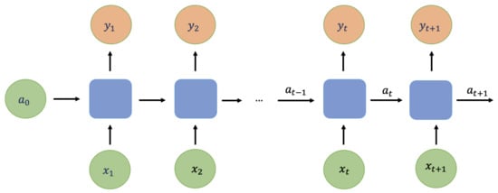
Figure 8.
An example of the recurrent neural network. represents the input of time t, is the output of time t, and is the hidden layer at time t.
For each t, the hidden layer and the output are as follows:
where , , , , and are coefficients that are shared temporally, and , are activation functions. is the activation function at the hidden layer and is the activation function at the output layer. Commonly used activation functions for RNN include sigmoid function, tan h function, etc.
We have previously introduced that mathematical formulas can be described as trees, and trees can be traversed as sequences. Figure 9 shows an example of how to describe the function using a sequence. We call each node in this sequence as tokens and denote the ith token in traversal as and the length of the traversal as . Each token has a value within the function set or the terminal set, and we combine these two sets together and call it the library L.

Figure 9.
An example of how to describe the function using a sequence expression.
Since mathematical formulas can be expressed using sequences, and the value of the previous token is obviously influential for the choices of the current token, it is straightforward for us to consider sampling the expression using a RNN. We will generate the expression in a way as shown in Figure 10.
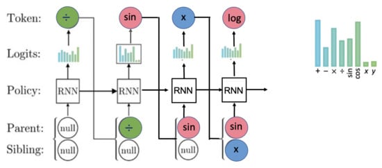
Figure 10.
Example of generating the first four tokens for the expression using RNN.
For each token, we use RNN to provide categorical distribution with parameters that define the probabilities of selecting each token from the library L, in this example, , where x and y are terminals, and others are functions.
After probabilities are generated, we sample a token. Then, the parent and sibling of the next token will be used as the next input of the RNN. Here, the parents and siblings represent the relationship between tokens we have currently generated. In our example, when we are trying to generate our fourth token, the third token x is the sibling of the second token . We keep this procedure until the tree is complete, that is, all tree branches reach terminal nodes. We call this generated expression the tree’s pre-order traversal.
Since the outputs of RNN here are categorical distributions that define the probabilities of selecting each token, the softmax function is used as the output layer activation function for the RNN. The softmax function is a function that turns a vector of real values into a vector of probabilities that sum to 1. That is, prior to applying softmax, the vector contains real numbers, but after applying softmax, each component will be in the interval , and the components will add up to 1 so that they can be interpreted as probabilities. Specifically, in our example, suppose we have L elements in the library, at state i (generate ith token), we use the softmax activation function to calculate the relative probabilities to each class:
where is the hidden layer with L dimension, represents the kth value of , and are the weights, for . In this way, we convert the hidden layer to , which takes a value between and represents the probability of choosing token j when we generate the ith token. For each state, weights remain the same. Here, Equation (4) represents the activation function at the output layer that we introduced in our RNN example in Equation (3), and are our outputs when generating ith token. The expressions are generated one token at a time using a categorical distribution that defines the probabilities of selecting each token from the library. Since the information about the expression that was previously generated is relevant, one needs to condition this probability upon the selections of all previous tokens. Specifically, conditioning the previously selected tokens , denotes the probability distribution for selecting the ith token .
where . Then, the probability of the whole expression is:
where represents weight parameters in RNN.
3.2.2. Constraints on Search Space
To effectively search the space of mathematical expressions, certain constraints need to be applied within the framework. These constraints are as follows: (1) The expressions are restricted to a pre-specified minimum and maximum length, which in this case is set to a range of 4 to 30. (2) The children of an operator should not all be constants, as the result would simply be a different constant. (3) The child of a one argument operator should not be the inverse of that operator, for example, is not allowed. (4) Descendants of trigonometric operators should not be trigonometric operators, for example, is not allowed. These constraints can be implemented by assigning a probability of zero to the selection of such tokens. This ensures that the model does not generate invalid expressions and allows for more efficient searching of the mathematical expression space.
3.2.3. Training RNN
Once a pre-order traversal is sampled, the corresponding mathematical expression will be evaluated with a reward function,
where is the normalized root mean square error, and is the expression described by .
Since the reward function in DSR is not differentiable with respect to , in Peterson et al. (2021), the risk-seeking policy gradients are introduced to train the RNN, and we can finally summarize the full procedure of the deep symbolic regression.
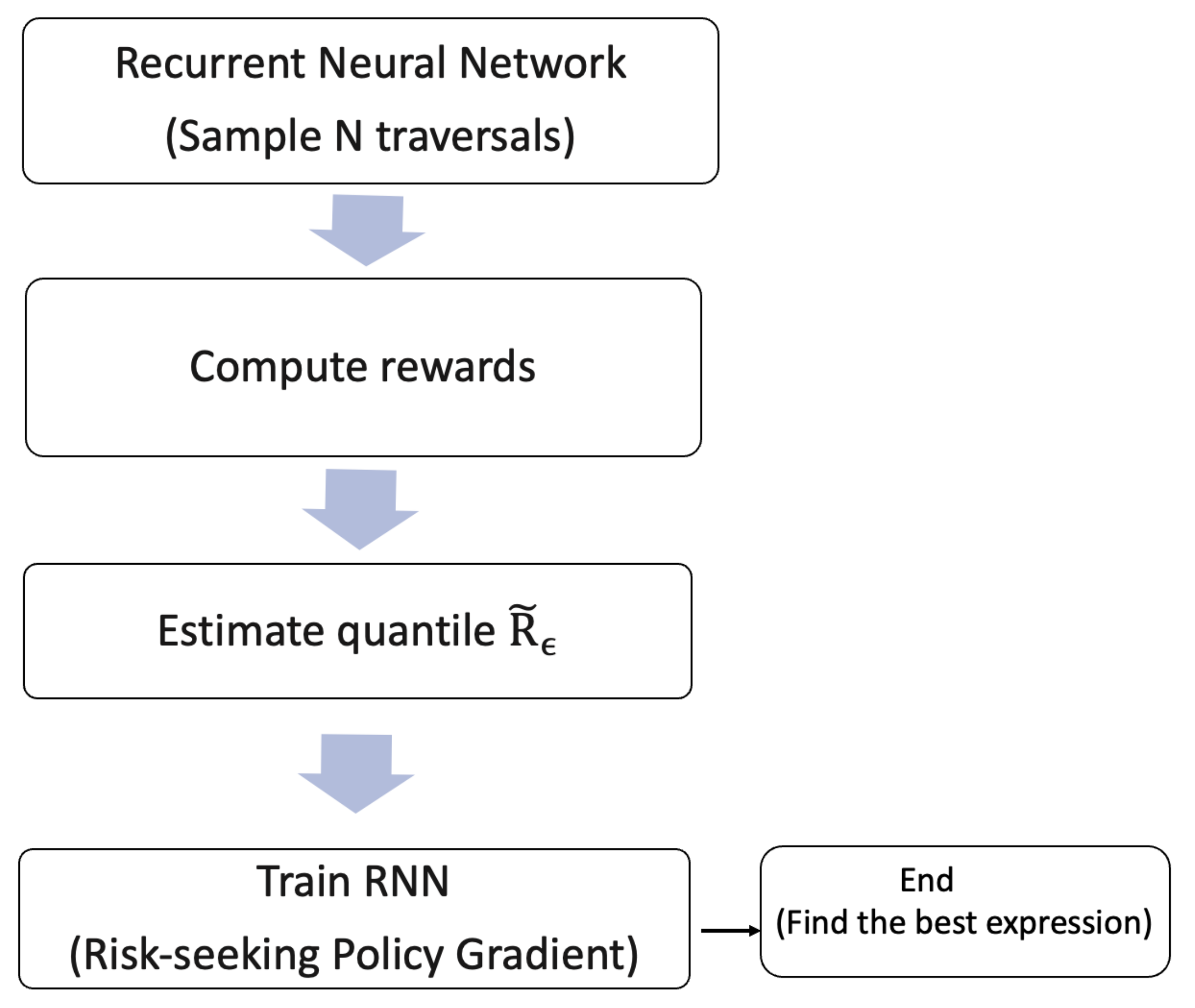
As shown in Figure 11, the whole procedure of DSR is as follows: (1) Use RNN to generate N expressions. (2) Calculate rewards for each of the expression. (3) Choose the subset of expressions that has rewards larger than the quantile of the rewards. (4) Use risk-seeking policy gradient to train the RNN and to update the best expression. The pseudocode for the DSR procedure is provided as Algorithm 1 in Peterson et al. (2021); we also include it in Appendix A.
| Algorithm 1 Basic pseudo-code for Bayesian optimization |
|
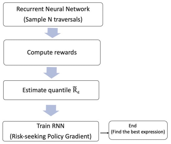
Figure 11.
Whole procedure of the deep symbolic regression.
4. Bayesian Optimization
In Section 3, we introduce the training method used in DSR. However, in GP-SR, there are additional hyperparameters to be tuned, such as tree depth, probabilities for each genetic operation, and population size. The traditional approach of parameter tuning, such as grid search, can be time-consuming. To overcome this, we have adopted Bayesian optimization (BayesOpt) to tune the hyperparameters of GP-SR. In this section, we will provide a detailed introduction to BayesOpt.
4.1. Overview of Bayesian Optimization
Bayesian optimization is a class of methods with a focus on solving the problem:
even though is hard to evaluate and lacks known special structure or lacks first or second order derivatives. This optimization method focuses on finding a global rather than local optimum. Hyperparameter optimization can be framed as the task of minimizing an objective score evaluated on the validation set, where x is the d-dimensional hyperparameters within the domain X. Common objective scores include RMSE, error rate, and so on. To accomplish this, Bayesian optimization can be a promising method for hyperparameter tuning.
Bayesian optimization has two main components: (1) a Bayesian statistical model that models the objective function, typically by applying a Gaussian process (GP) prior to the function of interest; (2) an acquisition function that determines the next sample point to evaluate. The complete procedure for BayesOpt can be found in Algorithm 1 of Frazier (2018) [11]; we also list it here as Algorithm 1.
4.2. Gaussian Process Regression
The first step of BayesOpt is to apply a Gaussian process prior to the function of interest. We first describe GP regression focusing on v’s value at a finite collection of points . For Gaussian process regression, we assume that the vector is prior to the multivariate normal distribution, i.e.,
where , and
Let us suppose that have no noise; at some new candidate point x, we can compute the posterior probability distribution as:
where
depending on the mean function in the prior , covariance function and the new candidate point.
The most common choice for for mean function is . We can also choose , where is a parametric function. For covariance function , we use a kernel at each pair of point and . The choices of kernel should have the property that each pair of that are closer in the input space should have a larger positive correlation, and the resulting covariance matrix is positive semi-definite. Some common choices of kernels are
- Power exponential kernel:where , and are parameters.
- Matern kernel:where is the modified Bessel function, and are parameters.
The mean function and kernel have parameters, which are called prior hyperparameters. One can always choose prior hyperparameters using maximum likelihood estimate (MLE). That is
where is the likelihood of the observations under the prior hyperparameters, and represents the set of prior hyperparameters. For example, if we assume constant mean and power exponential kernel, .
4.3. Acquisition Functions
Once the Gaussian process regression prior to the function of interest has been defined, the next step in BayesOpt is to use an acquisition function to determine the next point to sample. In this section, we will focus on introducing the most commonly used acquisition function, which is the expected improvement.
For simplicity, here we assume that the function of interest is noise free. Suppose we have evaluated n times thus far; then, indicates the point sampled at iteration m, and the optimal observed value is . Now suppose we want to evaluate using an additional point x; after this evaluation, the new optimal observed value is , and the improvement of this new evaluation should be , where . We can define the expected improvement as:
Here, indicates the expectation under the posterior distribution given the evaluations of at . This posterior distribution is normally distributed with mean and variance . We will choose to sample next where
One advantage of is that it can be evaluated in a closed form, which has first- and second-order derivatives. The closed form can be shown as below:
Here, and represent the cumulative distribution function and density function of a standard normal distribution, respectively. We can use a continuous first- or second-order optimization method (quasi-Newton, etc.) to solve .
Apart from the expected improvement, there are other acquisition functions that are widely used, such as the knowledge gradient and the upper confidence bound.
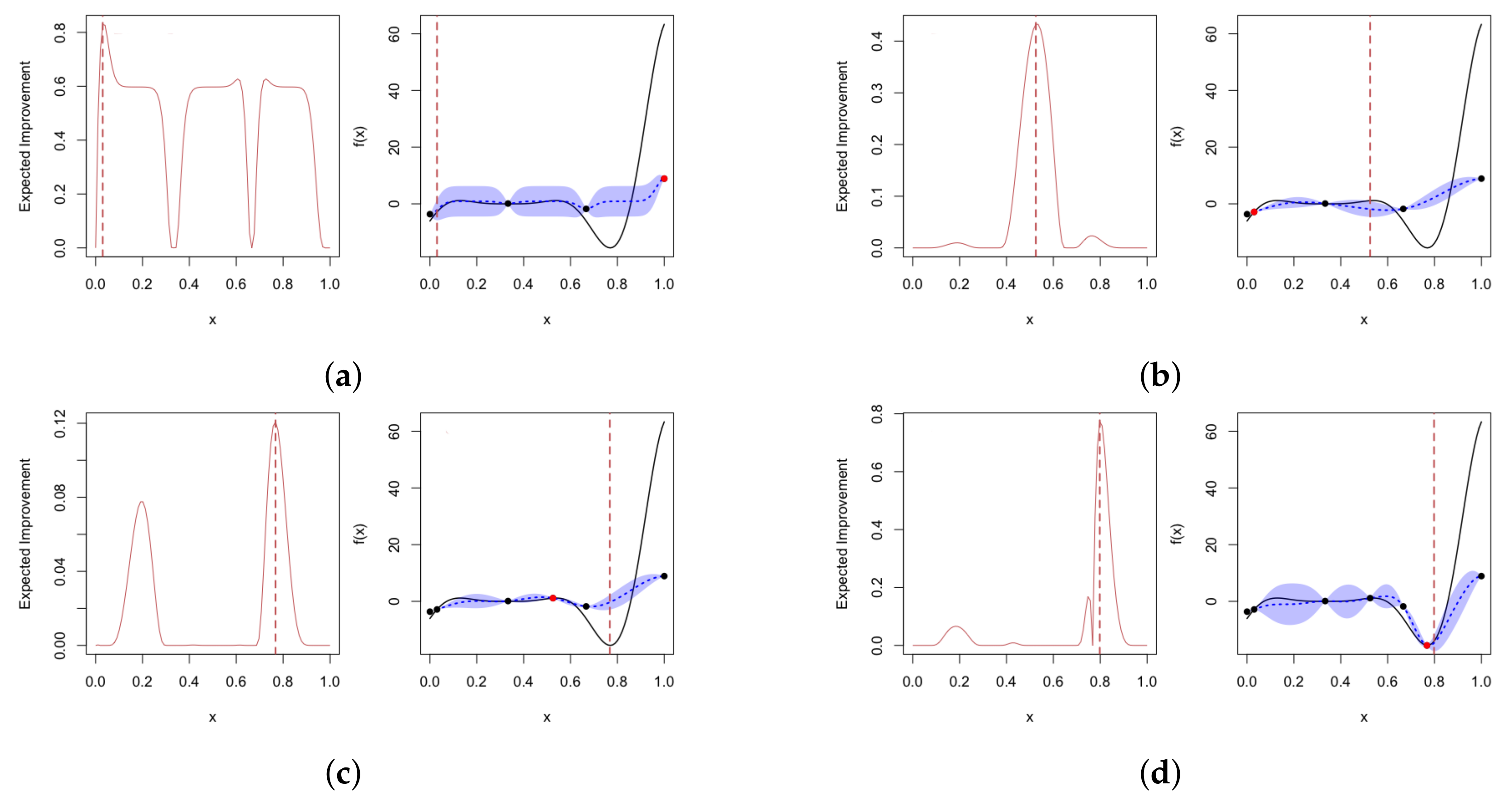
In Figure 12, we provide a simple illustration of Bayesian optimization. In this example, we aim to maximize the continuous function with one-dimensional input. At the start of optimization, we have three data points. Each subplot depicts (black solid line) in the top panel, with credible intervals for obtained using the Gaussian process posterior represented by blue shadows. The left panel shows the acquisition function, with the expected improvement used in this example. At each iteration, we choose the next sample point that maximizes the expected improvement, as indicated by the red dots on the black solid line. After four iterations, we identify the global optimum, as no further point can be selected to improve the score.
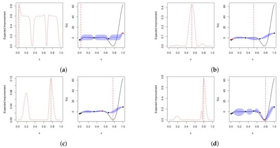
Figure 12.
An example of Bayesian optimization on a target function with four iterations, using the expected improvement as the acquisition function. The right panel in each sub-plot shows the noise-free objective function at 3, 4, 5 and 6 points (black dots). The solid black line represents true , and blue shadows show Bayesian credible intervals for . The left panel shows the acquisition function. In each iteration, we choose to sample the point that maximizes the acquisition function, which are shown using red dots on black solid lines. (a) First iteration; (b) second iteration; (c) third iteration; (d) fourth iteration.
5. Simulation Study
In the previous sections, we introduced two approaches for symbolic regression as well as methods for tuning their parameters. In this section, we evaluate the performance of these approaches through simulation studies to determine whether they can accurately identify the true relationships between inputs and outputs in a given dataset.
We simulated data using the following five “true” relationships:
- Simulation 1: ;
- Simulation 2: ;
- Simulation 3: ;
- Simulation 4: ;
- Simulation 5: ;
where represents the noise we add to our simulations.
The objective of Simulation 1 is to replicate the relationship between IVS, moneyness, and time to maturity based on the call and put implied volatilities observed on 2 May 2000, as detailed in Figure 1 of Fengler et al. [12]. In this simulation, we set , which aligns with the observed range. Similarly, the range for time to maturity is set as , which is generally within the observed range of time to maturity (days/365). The response range for is set at . A 3D surface plot for Simulation 1 is presented in Figure 13, where we can observe the smile curves when is fixed, even though it is not as complex as the IVS observed in practice.
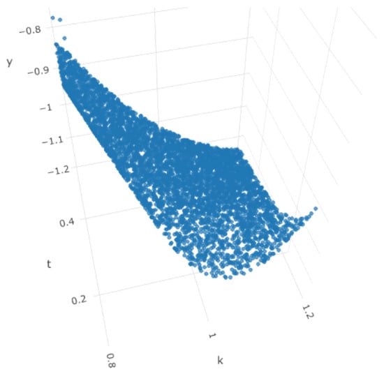
Figure 13.
Surface plot for Simulation 1 with no noise. x-axis represents the simulated k, y-axis represents simulated , and z-axis represents the simulated .
The remaining simulations aim to evaluate the effectiveness of symbolic regression in detecting specific mathematical terms of two parameters. Simulation 2 focuses on testing and polynomials nested in , while Simulation 3 tests exponential and polynomial equations. Simulation 4 evaluates the ratio of logarithms and square roots, and Simulation 5 tests a simple polynomial relationship.
We generated 3000 observations for each simulation configuration with varying noise levels. To evaluate the performance of each simulation, we started with and incrementally increased it from 0, 0.005, 0.01 to 0.1, until the method failed to detect the true mathematical relationship. We tuned the following parameters for GP-SR:
- Genetic Operation Probabilities: “p crossover”, “p subtree mutation”, “p hoist mutation” “p point mutation”;
- Population Size: Number of expression trees we generated in the initial population;
- Initial Method: The method we use to generate the initial population;
- Parsimony Coefficient: The parameter that controls the complexity levels of the proposed equations.
We used the “gplearn” module in Python to apply GP-SR and to employ the “skopt” module to apply Bayesian optimization to tune the genetic operation probabilities, population size, and initial method for GP-SR. For the parsimony coefficient, we only tested values of 0.005 and 0.01 in this simulation study. For the remaining parameters in GP-SR, we used the default values. The “initial depth” was set to , which specified the range of initial depths for the first generation of expression trees. The “population size” was set to 2000, which controlled the number of expression trees competing in each generation.
For deep symbolic regression (DSR), we utilized a Python module called “deep symbolic optimization”, developed by Brenden K Petersen, which is based on Petersen et al. [8]. We used default hyperparameter values for learning rate and the number of layers for RNN.
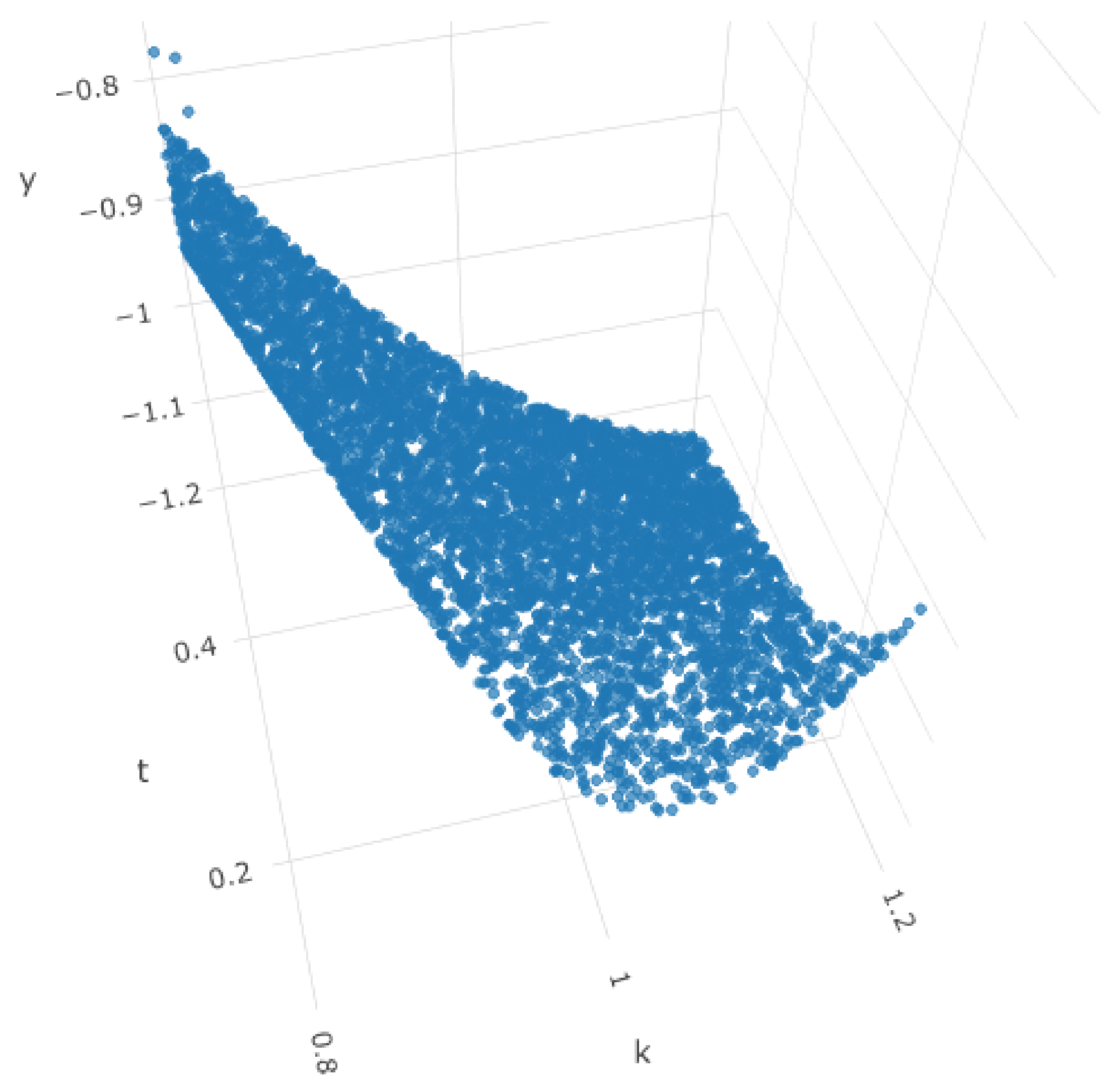
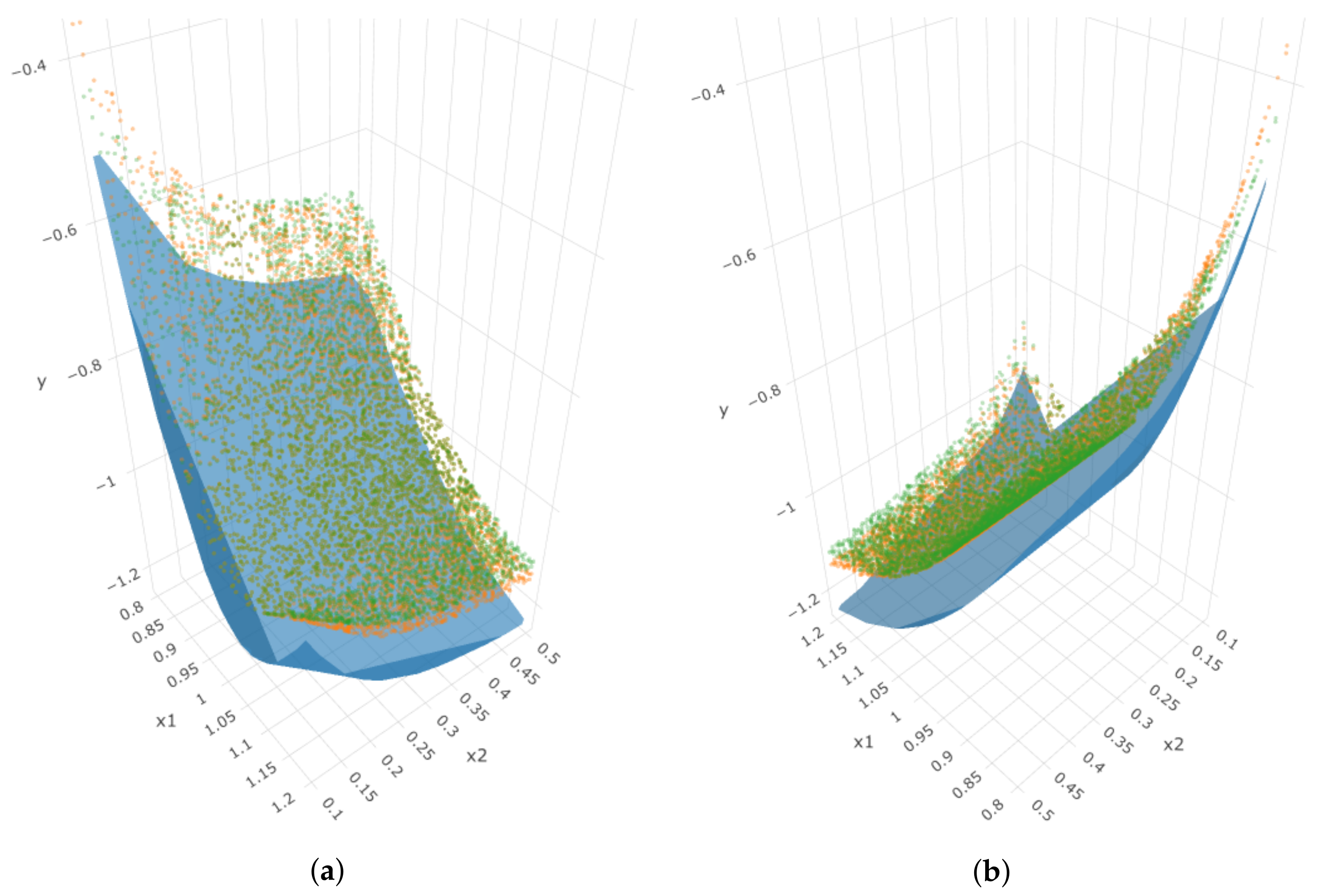
For Simulation 1, when we have , both GP-SR and DSR can successfully detect the true mathematical function, that is . However, when we increased to , both methods failed to detect it. Functions detected by GP-SR and DSR are shown in Table 1. Both of the methods at least successfully detected the term and . Figure 14 depicts two angles of the 3D plot of IVS, k and . The blue surface represents the true simulated IVS, while the dots with different colors represent the estimated implied volatility obtained by the two “wrong” functions proposed by each method. The results obtained by the two approaches are quite similar, with both being moderately far from the true simulated surface. The RMSE values for the estimated volatility obtained by each method and the true simulated implied volatility are displayed in Table 1.

Table 1.
Equations detected and their RMSEs for Simulation 1 for two methods with various noise levels.

Figure 14.
Two angles of the 3D plot for Simulation 1 when . The blue surface represents the true simulated surface, orange dots represent estimations using GP-SR, and green dots represent estimations using DSR. (a) First angle; (b) second angle.
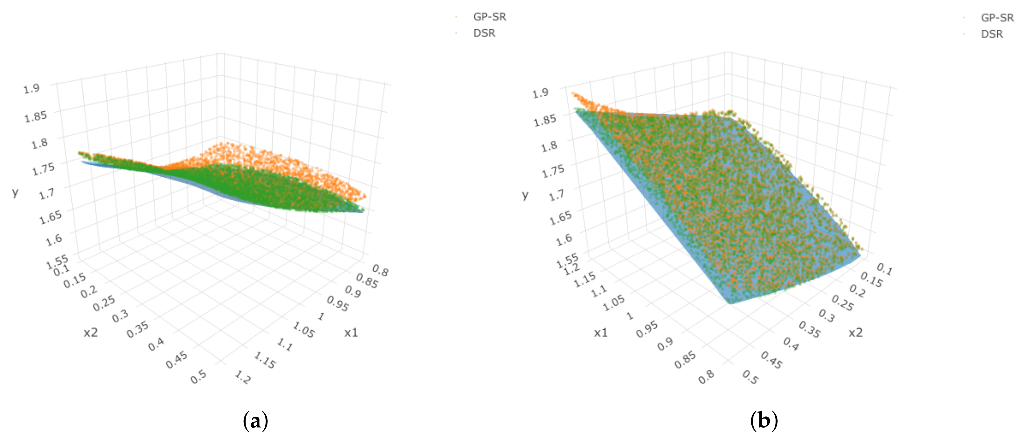
For Simulation 2, when we have , both GP-SR and DSR can successfully detect the true mathematical function, that is . However, when we increased to , both methods failed. Functions detected by GP-SR and DSR are shown in Table 2. Both of the functions detected the term but failed to detect . Figure 15 shows two angles for the 3D plot of y, and . The blue surface is the true simulated response surface, and dots with different colors represent the estimated response given by the two “wrong” functions proposed by the different methods. In this simulation, the results given by the GP-SR function are further away from the true surface than those given by DSR. The RMSE values between estimated volatility by both approaches and the true simulated implied volatility are small, as shown in Table 2.

Table 2.
Equations detected and their RMSEs for Simulation 2 for two methods with various noise levels.
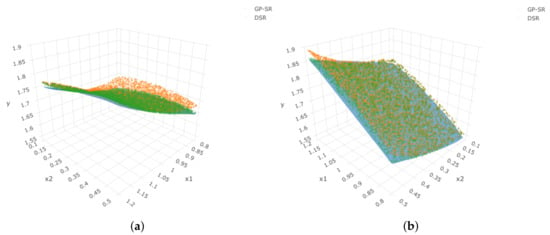
Figure 15.
Two angles of the 3D plot for Simulation 2 when . In each sub-plot, the blue surface represents the true simulated surface, orange dots represent estimations using GP-SR, and green dots represent estimations using DSR. (a) First angle; (b) second angle.
For Simulation 3, when we have , GP-SR can successfully detect the true mathematical function, that is , and it failed when increased to . The function GP-SR is identified as
which is also shown in Table 3. However, DSR can only detect the true function when . For , it cannot propose the exact same function as the true function in the simulation. The functions’ DSRs provided under different noise levels are shown in Table 3.

Table 3.
Equations detected and their RMSEs for Simulation 3 for two methods with various noise levels.
Both methods successfully detected the term even with but failed to detect . Figure 16 displays two angles of the 3D plot of y, and . The blue surface represents the true simulated response surface, while the dots with different colors represent the estimated responses obtained by the four “wrong” functions proposed by each method with different levels of noise. From Figure 16, we can see that the estimations obtained using DSR under are nearly identical to the true responses (blue surface), indicating that DSR can be highly sensitive to even small amounts of noise in the data. Thus, in this case, we may still consider that DSR has detected the “true” surface. Comparing DSR and GP-SR, even though DSR failed to detect the true function at lower noise levels, the results obtained by DSR are closer to the true surface than those from the GP approach when . In this case, DSR performs better under relatively higher noise levels. The RMSE values for the estimated responses obtained by each method and the true simulated responses are provided in Table 3.
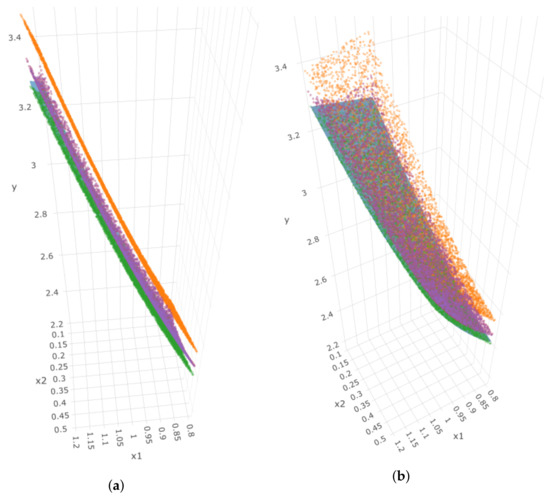
Figure 16.
Two angles of the 3D plot for Simulation 3, where x-axis represents , y-axis represents , and z-axis represents our simulated response. In each sub-plot, the blue surface represents the true simulated surface, orange dots represent estimations using GP-SR, and dots of other colors represent estimations using DSR with different noise levels. (a) First angle; (b) second angle.
In Simulation 4 and Simulation 5, as we increase the noise level from 0 to 0.1, both GP-SR and DSR can successfully detect the true mathematical relationships between inputs and output. The RMSE values for the estimated responses obtained by each method and the true simulated responses are provided in Table 4 and Table 5, respectively.

Table 4.
Equations detected and their RMSEs for Simulation 4 for two methods with various noise levels.

Table 5.
Equations detected and their RMSEs for Simulation 5 for two methods with various noise levels.
These simulation results demonstrate that both symbolic regression methods are effective in detecting the true mathematical relationships between inputs and outputs when the noise levels are low. However, as the noise levels increase, both methods may fail. In the case of more complex mathematical forms (Simulation 1), even a small amount of noise can cause both methods to fail. However, when dealing with simpler mathematical equations (Simulation 4 and Simulation 5), both methods can perform well even with higher noise levels.
All of the previous conclusions were based on a single trial of simulations for each setting, and we kept the number of observations fixed at 3000. What if we decrease the number of observations, will these methods succeed under the same noise level? Or if we increase the number of observations, will both methods tolerate higher noise level? To answer these questions, we tried more combinations of number of observations n and noise levels for each of the simulation settings.
Specifically, we first fixed and tried ; then, we fixed and tried . For each simulation setting, we ran 100 trials and calculated the return rates () for each method.
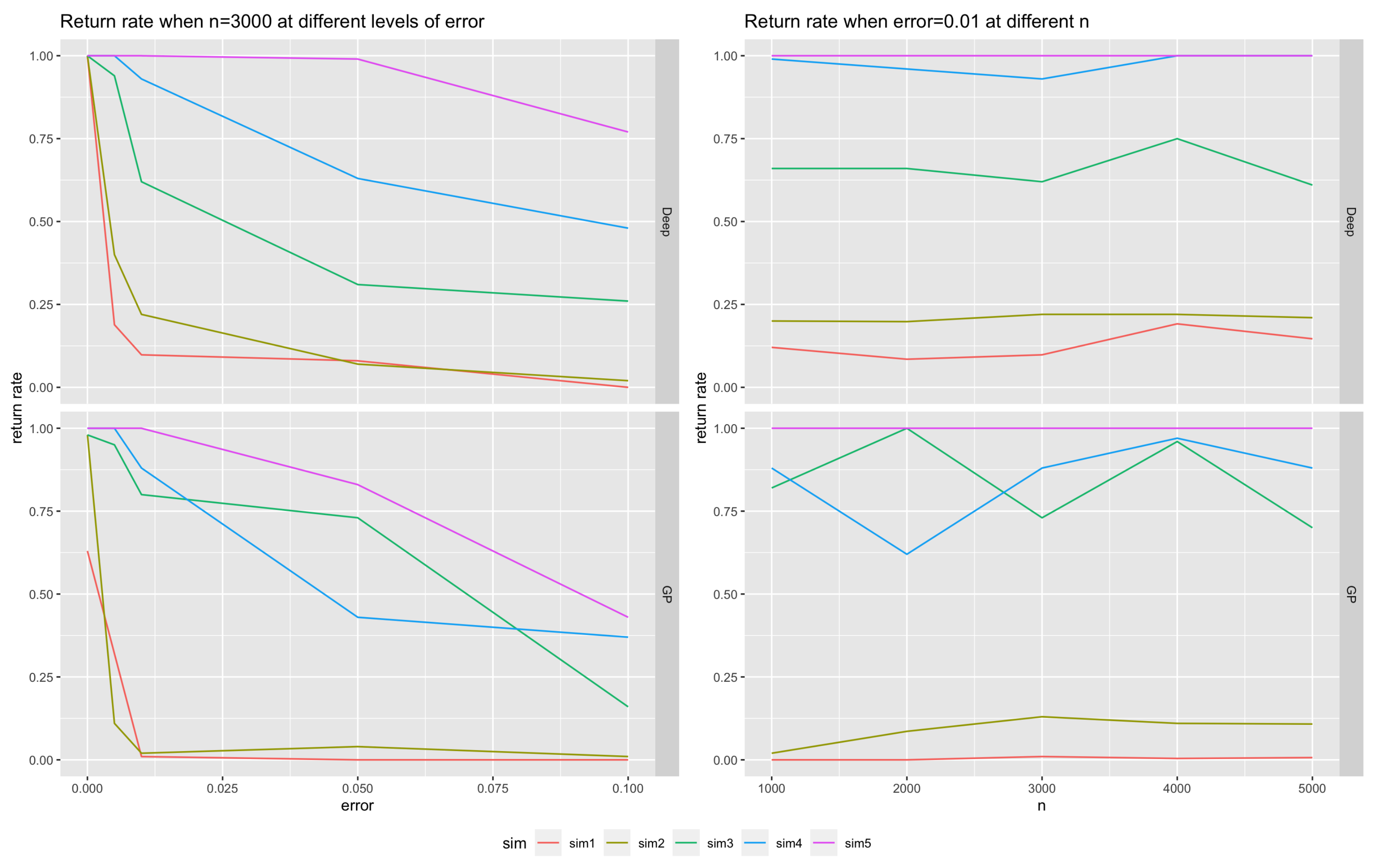
Figure 17 presents the return rates for the two approaches across different simulation settings. The left panel displays the return rates for as increases from 0 to 0.1, while the right panel shows the return rates for as n varies from 1000 to 5000. The numeric results are also summarized in Table 6 and Table 7. The findings indicate that across all five simulation set ups, the return rates decrease as the noise level increases for both approaches. For the more complex equations (Simulation 1 and Simulation 2), the return rates plummet when and , with GP-SR exhibiting particularly poor performance, with return rates approaching zero when . However, for simpler simulations, such as Simulation 5, both approaches show a slower decrease in return rates. In general, DSR outperforms GP-SR by providing higher return rates at the same noise levels. The only exception is Simulation 3, where GP-SR performs slightly better than DSR when , which suggests that GP-SR may be more effective in detecting the mathematical term .
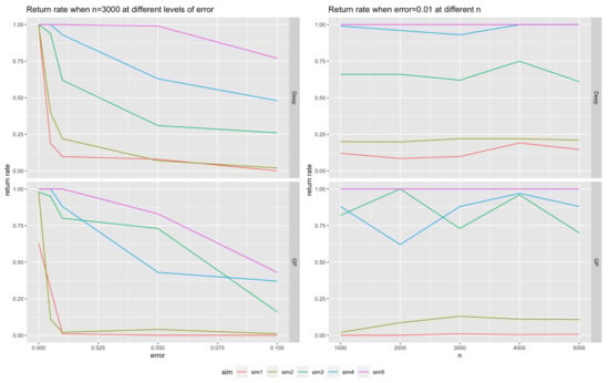
Figure 17.
Return rates: The left panel shows the return rates for two approaches when , where the x-axis represents the and y-axis represents return rates. The right panel shows the return rate for the two approaches when , the x-axis represents n, and the y-axis represents return rates. Within each panel (left or right), the top plot shows return rates using DSR, and the bottom plot shows return rates using GP-SR. Within each sub-plot, different colors represent five different simulation equations.

Table 6.
Return rates from both methods at different noise levels when n = 3000.

Table 7.
Return rates from both methods at different number of observations when .
When we fixed and increased the number of observations n, there was no clear and stable trend in the changes in return rates for the same simulation type. This implies that the performances of both methods are more influenced by the complexity of the “true” relationships and noise levels and are less influenced by the size of the data, provided that .
6. Empirical Study
In the simulation study, we found that both GP-SR and DSR methods perform well when the noise level is limited. However, as the noise level increases, both methods start to struggle in detecting the true relationship between inputs and outputs, even if they produce similar RMSEs. Moreover, both methods may fail with extremely small noise if the relationship between inputs and outputs is overly complex.
In this section, we evaluate the performances of two symbolic regression approaches using daily options data on the S&P 500 index. The dataset comprises 1829 days of call and put options, spanning from 2 January 2015 to 16 April 2022, and covering a diverse range of maturities and moneyness.
Following the rules described in Gao et al. [13], we began by cleaning the data. First, we considered only options with a maturity greater than 7 days but less than a year. Second, we only considered options with a bid price greater than dollars. Third, we removed options with a bid price larger than the offer price. Finally, we eliminated options with no implied volatility or negative prices.
Note that the implied volatility surface varies for different times t and types of options (put or call). For most dates, we had more put options data than call options data. We selected four dates with the most put options data, namely, 21, 25, 26, and 27 January 2022, and evaluated the performance of the two symbolic regression approaches in identifying the relationship between IVS, moneyness, and time to maturity using daily data separately.
For the ith option in date t, let us denote
- represents time to maturity (days/365);
- represents moneyness, . Here, represents the strike price, is the risk-free interest rate at date t, represents time to maturity, and represents the underlying price of the asset.
For each date, we used and as inputs and used both GP-SR and DSR together with the Bayesian optimization method to find mathematical models that can provide a good estimation for the implied volatility surface .
Goncalves et al. [14] proposed a model that performs very well in estimating IVS. Based on their years of financial experience, they proposed adjusting moneyness using time to maturity . Precisely, they used instead of raw moneyness in the model. After adjustment, they fit the log-transformed volatility on a daily basis using a polynomial model as the following:
We used this model as a benchmark and compared the equations obtained through symbolic regressions with the benchmark model, using RMSE and correlations between predicted implied volatility and true implied volatility as metrics of comparison.
On the date of 21 January 2022, there were 3227 put options available. Using BayesOpt to tune the parameters for both GP-SR and DSR, we obtained the following equations:
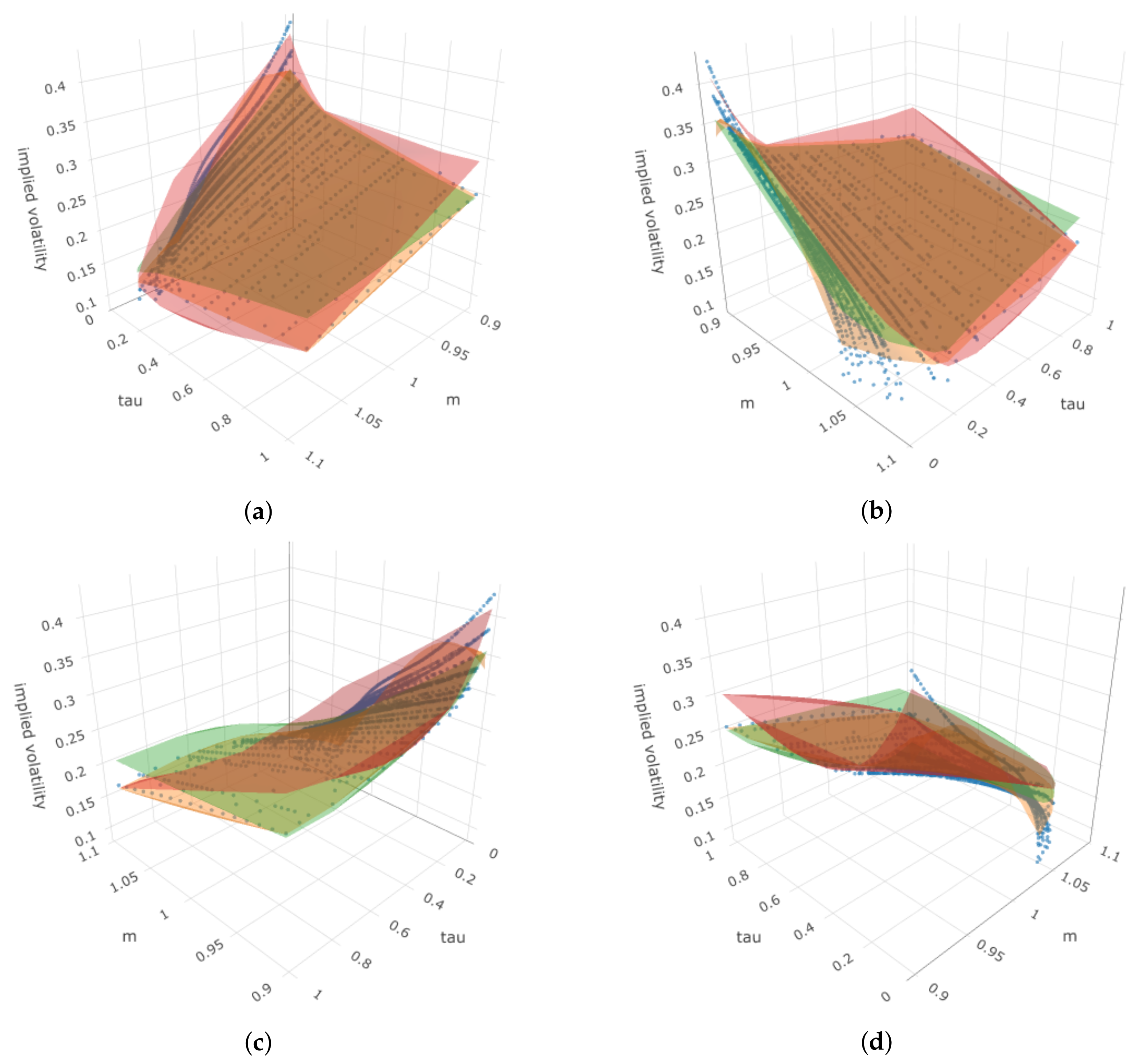
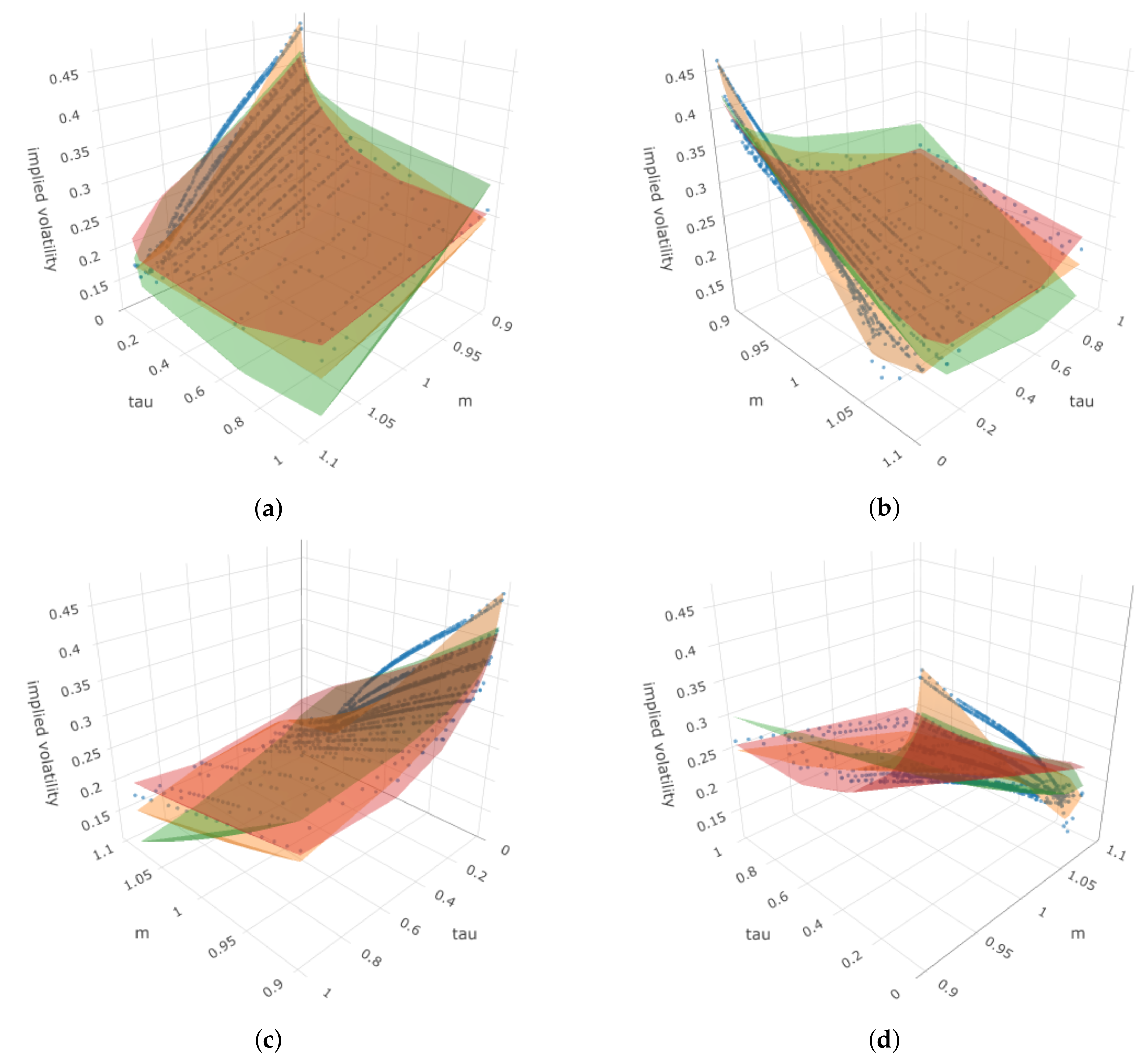
After these two equations were detected, we calculated the estimated implied volatility for each option and computed the correlation and RMSE for . The results are shown in Table 8. From Table 8, we can see that the benchmark model provides the highest correlation and lowest RMSE. Among GP-SR and DSR, GP-SR performs better. Figure 18 presents four angles for the 3D plot of IVS, moneyness k, and time to maturity . The blue dots represent the true observed implied volatility, and the surfaces with different colors represent the estimated implied volatility surfaces using different methods. From Figure 18, we can see that when we fix , the observed implied volatility generally increases as moneyness increases (third angle). However, when we fix the moneyness at different values, we can see obvious curves with smile shapes that move in different directions as time to maturity increases (fourth angle). All three methods can successfully capture these differences in directions.

Table 8.
Summaries of results for four dates: the top table shows correlations between estimated implied volatility and observed implied volatility for each date using three different methods. The bottom table shows RMSEs. (a) Correlations for different models; (b) RMSE for different models.

Figure 18.
Four angles of the 3D plot for put options in 21 January 2022, where the z-axis represents the implied volatility. In each sub-plot, blue dots represent the true observed implied volatility, the orange surface represents estimated IVS using Benchmark, the red surface represents estimated IVS using DSR, and the green surface represents estimated IVS using GP-SR. (a) First angle; (b) second angle; (c) third angle; (d) fourth angle.
For the date of 25 January 2022, there are 1292 put options available, and the equations detected by GP-SR and DSR are as follows. The numeric results are shown in Table 8.
Upon analyzing the results for the date 25 January 2022, it can be observed that the benchmark model outperforms GP-SR and DSR, with the latter two methods exhibiting comparable performance but slightly worse than the benchmark. Notably, the equation obtained by DSR is overly complex, while the one detected by GP-SR is significantly simpler but yields comparable results.
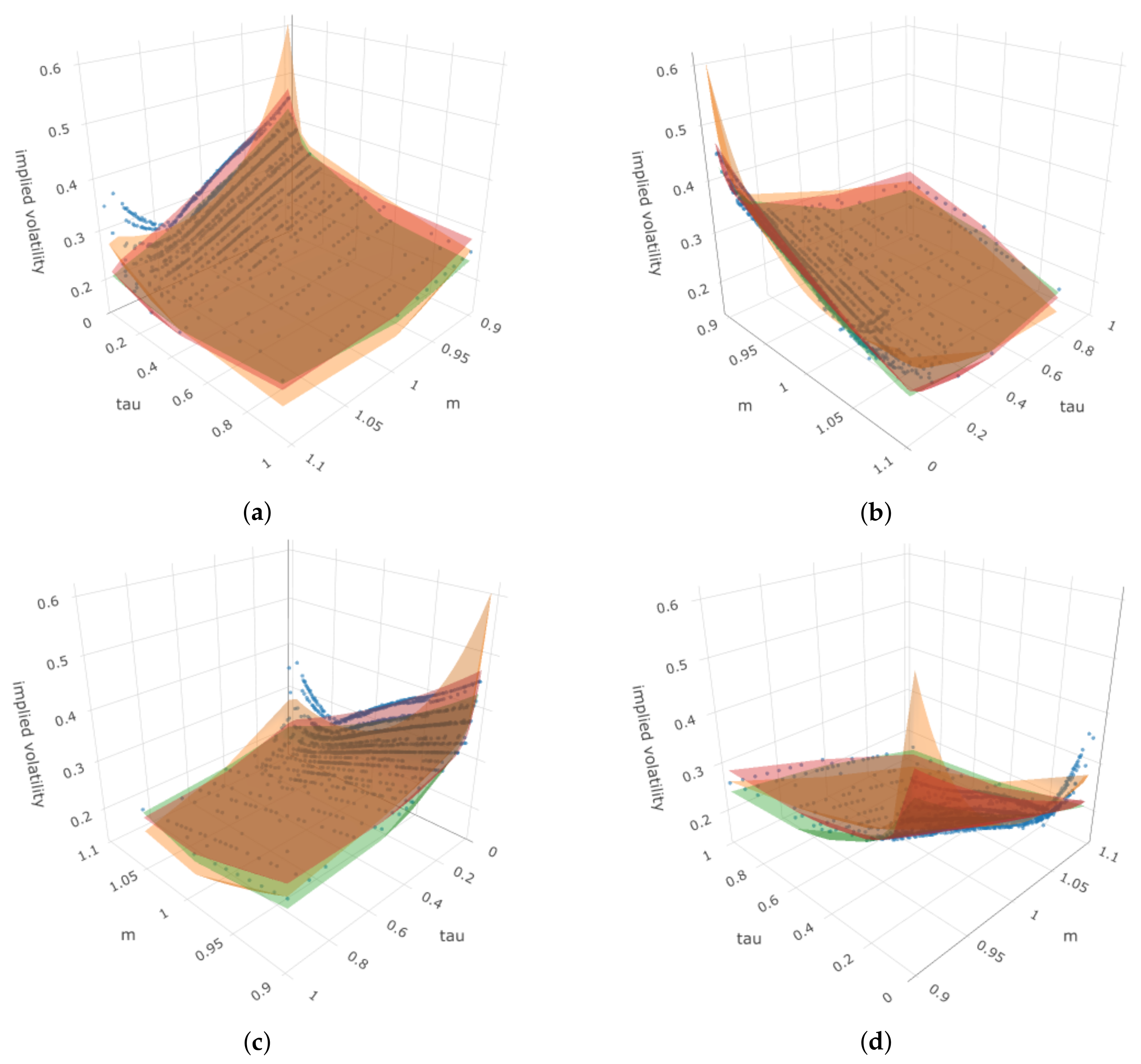
Figure 19 depicts the 3D plot from four angles, where the blue dots indicate the true observed implied volatility and the surfaces with different colors represent the estimated implied volatility surfaces using the three different methods. We observed some similar patterns to those from the previous date of 21 January 2022. However, we note that only the benchmark model can slightly detect the different directions for the smile curves when we fix the moneyness at different values (fourth angle).
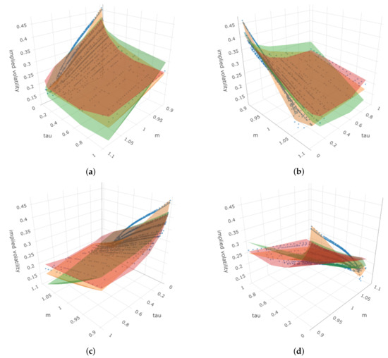
Figure 19.
Four angles of the 3D plot for put options on 25 January 2022, where the z-axis represents the implied volatility. In each sub-plot, blue dots represent the true observed implied volatility, the orange surface represents estimated IVS using benchmark, the red surface represents estimated IVS using DSR, and the green surface represents estimated IVS using GP-SR. (a) First angle; (b) second angle; (c) third angle; (d) fourth angle.
For the date 26 January 2022, there are 1407 put options available. The equations detected by GP-SR and DSR are as follows, and the numeric results are shown in Table 6:
On this date, both symbolic regression methods produce comparably complex equations, but they outperform the benchmark model. Among GP-SR and DSR, DSR performs better. Figure 20 shows that for this date, there are no clear differences in directions for the smile curves when we fix the moneyness at different values, and both symbolic regression methods perform better than before.

Figure 20.
Four angles of the 3D plot for put options in 26 January 2022, where the z-axis represents the implied volatility. In each sub-plot, blue dots represent the true observed implied volatility, the orange surface represents estimated IVS using benchmark, the red surface represents estimated IVS using DSR, and the green surface represents estimated IVS using GP-SR. (a) First angle; (b) second angle; (c) third angle; (d) fourth angle.
For this date, both symbolic regression methods outperform the benchmark model. While the DSR performs slightly better than GP-SR, its equation is overly complicated. In contrast, GP-SR provides an equally good performance with a simpler equation. Figure 21 illustrates that when fixing moneyness at different values, we observe slightly different directions for the smile curves. Nonetheless, both symbolic regression methods still outperform the benchmark.
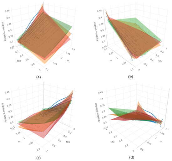
Figure 21.
Four angles of the 3D plot for put options in 27 January 2022, where the z-axis represents the implied volatility. In each sub-plot, blue dots represent the true observed implied volatility, the orange surface represents estimated IVS using Benchmark, the red surface represents estimated IVS using DSR, and the green surface represents estimated IVS using GP-SR. (a) First angle; (b) second angle; (c) third angle; (d) fourth angle.
The results from the four single days show that there is no consistent conclusion on which method performs the best. Generally speaking, sometimes DSR provides the highest correlations and lowest RMSEs, but it tends to produce overly complicated mathematical equations. GP-SR can sometimes provide parsimonious models with equally good performances, and other times, it is the benchmark model that works the best.
For the final date, 27 January 2022, there are 1308 put options available. The equations detected by GP-SR and DSR are presented below, and the corresponding numeric results are shown in Table 6.
Thus far, we have only analyzed daily put options data separately. However, Goncalves et al. [14] applied their model on a daily basis by re-estimating coefficients and the IVS using the same model structure for each date. The previous exploration based on the four dates provides insight into the functional forms suggested by GP-SR and DSR. Based on some of the equations discovered for those four dates, we attempted to fit each day of the following four non-linear models to the implied volatility data every day over all 1829 different dates.
For each date t, fit the following four non-linear models on put options separately. Here, i represents the ith option in date t;
- Model 1 (Based on the GP-SR equation in 21 January 2022):
- Model 2 (Based on the GP-SR equation in 25 January 2022):
- Model 3 (Based on the GP-SR equation in 26 January 2022):
- Model 4 (Based on the GP-SR equation in 27 January 2022):
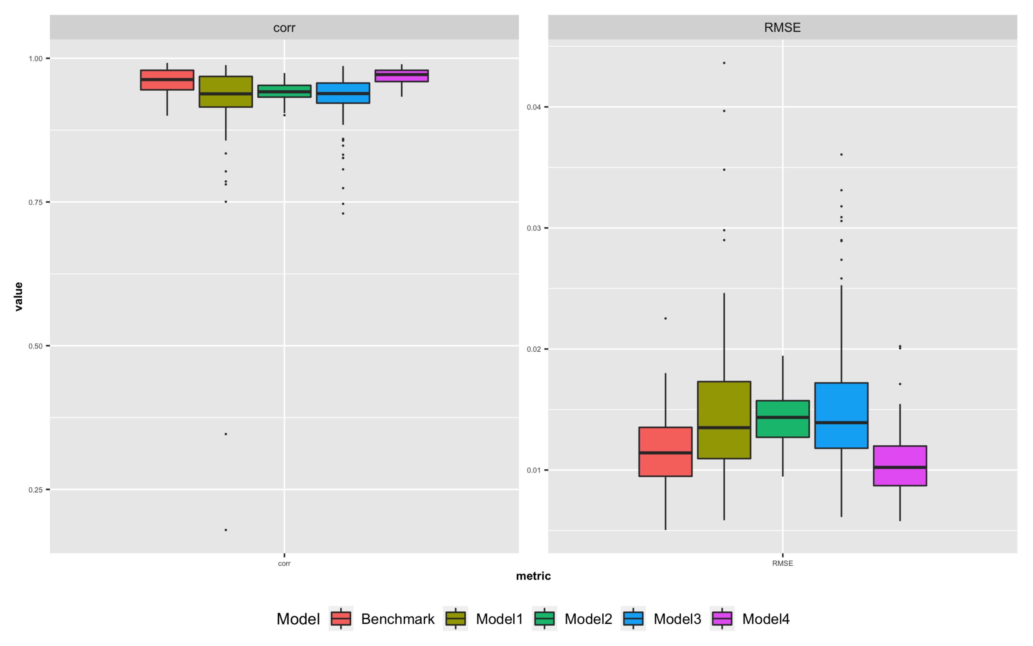
We applied the four non-linear models and the benchmark model to daily implied volatility data for all 1829 dates. We calculated the RMSE and correlation between predicted and observed implied volatility for each date using each method. The results are summarized in Table 9 and are shown in Figure 22, where box plots of the 1829 daily RMSE and correlation values for all five models are presented.

Table 9.
The results for different models using daily data. (a) RMSE summaries for the four proposed models and the benchmark model using 1829 daily put options. The RMSE between predicted implied volatility and observed volatility using each model is calculated for each date. The table shows the mean, standard deviation and quantiles of the 1829 daily RMSEs for each model. (b) Correlation summaries for the four proposed models and the benchmark model using 1829 daily put options. The RMSE between predicted implied volatility and observed volatility using each model is calculated for each date. The table shows mean, standard deviation and quantiles of 1829 daily correlations for each model.
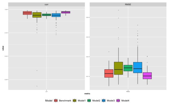
Figure 22.
Box plots for 1829 daily RMSE and correlations using four proposed methods and the benchmark. The left panel shows box plots for the correlations between estimated IVS and true IVS for 1829 dates. The right panel shows box plots for the RMSEs between estimated IVS and true IVS for 1829 dates. Different colors represents results for different methods.
The box plots and summary tables show that Model 4 outperforms the Benchmark in terms of providing smaller RMSEs and higher correlations between estimated and observed implied volatility. However, all other methods perform worse than the benchmark. Additionally, we analyzed the stability of the parameter estimates for Model 4 and found that they are generally consistent across all 1829 dates, as summarized in Table 10.

Table 10.
Summaries for 1829 sets of parameter estimates for Model 4.
Model 4 outperforms the benchmark model in terms of providing smaller RMSEs and higher correlations between estimated implied volatility and observed implied volatility. Additionally, unlike the linear model addressed in Dumas, Fleming, and Whaley [1] and the non-linear GARCH(1,1) model proposed by Heston and Nandi [3] in which coefficient estimates are highly unstable, Model 4 provides stable coefficient estimates across all 1829 dates of put options data. However, the major disadvantage of Model 4 is that the form of the model may be too complicated for economists to explain. Nevertheless, this result indicates that using symbolic regression can potentially propose meaningful mathematical relationships between IVS, moneyness, and time to maturity, even without deep understanding of financial theories. It may also provide insights into what might possibly be a good feature for modeling IVS. For instance, Model 2 is a linear regression on two simple transformations, namely and . Although this model does not perform as well as the benchmark, it still has decent performances. This could be evidence that and may be good features for predicting the implied volatility surface.
7. Conclusions
This paper introduces two symbolic regression (SR) approaches, GP-SR and DSR, to address the financial question of modeling implied volatility surface using moneyness and time to maturity. While SR methods have previously been successful in areas such as physics, this is the first time they have been applied to financial data with high noise levels. Through simulation studies, we learn that SR methods work well with low noise but can fail when noise levels increase or when the true relationship between inputs and output is too complex.
In the empirical study, we compare the performance of the SR methods with a fully developed benchmark model. The results show that the performances of SR methods are comparable with the ones of the benchmark model. Additionally, we discovered a universal non-linear model that can be applied to options data on a daily basis with stable coefficient estimates that has better performances than the benchmark model. However, the model may be too complicated to integrate.
Nonetheless, the empirical study shows that SR methods have the potential to help us discover meaningful relationships between IVS, moneyness, and time to maturity even without a deep understanding of financial theories. Furthermore, SR methods can potentially identify good features for IVS prediction.
Author Contributions
Conceptualization, J.L. and C.L.Y.; Methodology, J.L. and C.L.Y.; Formal analysis, J.L.; Investigation, C.L.Y.; Writing—original draft, J.L. and C.L.Y.; Writing—review & editing, J.L. and C.L.Y.; Visualization, J.L.; Supervision, C.L.Y. All authors have read and agreed to the published version of the manuscript.
Funding
This research received no external funding.
Data Availability Statement
Data sharing not applicable.
Conflicts of Interest
The authors declare no conflict of interest.
Appendix A. Pseudocode for Deep Symbolic Regression
| Algorithm A1 Deep symbolic regression with risk-seeking policy gradient |
|
References
- Canina, L.; Figlewski, S. The informational content of implied volatility. Rev. Financ. Stud. 1993, 6, 659–681. [Google Scholar] [CrossRef]
- Dumas, B.; Fleming, J.; Whaley, R.E. Implied volatility functions: Empirical tests. J. Financ. 1998, 53, 2059–2106. [Google Scholar] [CrossRef]
- Heston, S.L.; Nandi, S. A closed-form GARCH option valuation model. Rev. Financ. Stud. 2000, 13, 585–625. [Google Scholar] [CrossRef]
- Graves, A. Generating sequences with recurrent neural networks. arXiv 2013, arXiv:1308.0850. [Google Scholar]
- Schmidt, M.; Lipson, H. Symbolic regression of implicit equations. In Genetic Programming Theory and Practice VII; Springer: Boston, MA, USA, 2009; pp. 73–85. [Google Scholar]
- Evolutionary Computation 1: Basic Algorithms and Operators; Back, T., Fogel, D.B., Michalewicz, Z., Eds.; CRC Press: Boca Raton, FL, USA, 2018. [Google Scholar]
- Udrescu, S.-M.; Tegmark, M. AI Feynman: A physics-inspired method for symbolic regression. Sci. Adv. 2020, 6, eaay2631. [Google Scholar] [CrossRef] [PubMed]
- Petersen, B.K.; Landajuela, M.; Mundhenk, T.N.; Santiago, C.P.; Kim, S.K.; Kim, J.T. Deep symbolic regression: Recovering mathematical expressions from data via risk-seeking policy gradients. arXiv 2019, arXiv:1912.04871. [Google Scholar]
- Black, F.; Scholes, M. The pricing of options and corporate liabilities. J. Political Econ. 1973, 81, 637–654. [Google Scholar] [CrossRef]
- Koza, J.R.; Goldberg, D.E.; Fogel, D.B.; Riolo, R.L. Genetic Programming 1996: Proceedings of the First Annual Conference; Mit Press: Cambridge, MA, USA, 1996. [Google Scholar]
- Frazier, P.I. A tutorial on Bayesian optimization. arXiv 2018, arXiv:1807.02811. [Google Scholar]
- Fengler, M.; Hardle, W.; Mammen, E. A dynamic Semiparametric Factor Modelfor Implied Volatility String Dynamics; SFB 649 Discussion Paper; Humboldt University: Berlin, Germany, 2005. [Google Scholar]
- Gao, G.P.; Lu, X.; Song, Z. Tail risk concerns everywhere. Manag. Sci. 2019, 65, 3111–3130. [Google Scholar] [CrossRef]
- Goncalves, S.; Guidolin, M. Predictable dynamics in the S&P 500 index options implied volatility surface. J. Bus. 2006, 79, 1591–1635. [Google Scholar]
Disclaimer/Publisher’s Note: The statements, opinions and data contained in all publications are solely those of the individual author(s) and contributor(s) and not of MDPI and/or the editor(s). MDPI and/or the editor(s) disclaim responsibility for any injury to people or property resulting from any ideas, methods, instructions or products referred to in the content. |
© 2023 by the authors. Licensee MDPI, Basel, Switzerland. This article is an open access article distributed under the terms and conditions of the Creative Commons Attribution (CC BY) license (https://creativecommons.org/licenses/by/4.0/).

