Abstract
In this article, we consider the improved perturbed nonlinear Schrödinger Equation (IP-NLSE) with dual power law nonlinearity, which arises in optical fibers and photovoltaic-photo-refractive materials. We found grey and black optical solitons of the governing equation by means of a suitable complex envelope ansatz solution. By using the Chupin Liu’s theorem (CLT) for the grey and black solitons, we evaluated new categories of combined optical soliton (COS) solutions to the IP-NLSE. The propagation behaviors for homoclinic breathers (HB), multiwaves and M-shape solitons will be analytically examined. All new analytical solutions will be found by an ansatz function scheme and suitable transformations. Multiwave solitons have been reported by using a three-waves technique. Furthermore, two kinds of interactions for M-shape soliton through exponential functions will be examined.
MSC:
35J05; 35J10; 35K05; 35L05
1. Introduction
Optical solitons have been extensively applied in high-speed and high-capacity communication systems as an information carrier. The nonlinear Schrödinger Equation (NLSE) is one of the rarely used models in this context and describes the evolution in optics [1,2,3,4,5,6,7,8,9,10,11,12,13,14,15,16,17,18,19]. Recently, the study of exact rational solutions, their interactions, homoclinic breathers and multiwaves has been receiving attention from many scientists for their applications in biophysics, nonlinear fibers, oceanography and plasma. There are some adequate techniques that are applied to achieve the retrieval of rational solutions to the nonlinear systems [20,21,22,23,24,25,26,27,28,29,30,31,32,33,34].
The IP-NLSE in its dimensionless form is given as [35],
where x and t stand for the spatial and temporal variables, respectively, while is the soliton pulse profile. The 1st term interprets the linear evolution. The m stands for a nonlinearity factor that is applied to put the model into a generalized setting. represents the self-steepening perturbation term, while the coefficient of is the inter-modal dispersion and is the nonlinear dispersion coefficient. The coefficient of b accounts for the group velocity dispersion and the coefficient of a accounts for spatio-temporal dispersion and hence Equation (1) stays integrable. The coefficient c interprets the non-Kerr-law nonlinear term. Now, in order to use the functional F, it is important to consider the smoothness of . Treating the complex plane C as a two-dimensional linear space the function is continuously differentiable, so that
2. Dual-Power Nonlinearity
This nonlinearity is used in photovoltaic photorefractive materials such as [35],
where and are constants. Therefore, Equation (1) reduces to [35],
since for dual power law nonlinearity, . Furthermore, as expected, for , the dual power law changes to the parabolic law and Equation (4) will be entertained in the upcoming sections of the paper. Some researchers worked on the stated model. For instance, Biswas et al. investigated optical soliton perturbation via a trial function method [35] and Ekici et al. studied the analysis of solitons in nonlinear materials [36], but the motivation of this document is to find the grey and black optical solitons for the governing equation by means of a suitable complex envelope ansatz solution. With the application of CLT to the grey and black solitons, we evaluate new sets of COS for the model. Furthermore, we will discuss the propagation of homoclinic breathers, multiwaves and rational solitons [37,38,39].
The rest of the article is as follows: In Section 3, we will give the evaluation of grey and black optical solitons by using a complex envelope ansatz solution. Our Section 4 contains the CLT extended to optical solitons with its applications to the stated model. In Section 5, we will give the evaluation of COS of type-I and in Section 6 the evaluation of COS of type-II. In Section 7, we learn the multiwave solution for the governing problem via a three-waves scheme. In Section 8, the HB scheme is presented and we compute new solitons. In Section 9, we will form the rational solitons and their interactions in Section 10 and Section 11 respectively. Our Section 12, contains the discussions and finally our Section 13 contains the conclusion.
3. Grey and Black Optical Solitons (GBOS)
For these solitons, we apply the following transformation in Equation (4) [40],
where the is a complex function, stands for phase shift, v denotes the phase constant, represents frequency and represents wave number. To find GBOS for Equation (4), we choose [40]:
where v is pulse width and denotes inverse group velocity shift. The amplitude of is
and, furthermore, the nonlinear phase is
For in Equation (6), a dark soliton is known as a black soliton. However, for in Equation (6), a GOS is attained.
Solving distinct equations from the coefficients of tanh, and we find the following:
- Constants:
- :
- ::
- ::
- :
3.1. Type 1: Grey Optical Soliton (GOS) ()
The soliton will exist provided and .
3.2. Type 2: Black Optical Soliton (BOS) ()
4. Optical Solitons Extension via Chupin Liu’s Theorem (CLT)
The CLT shows a relationship among kink–bell and kink-type solutions [40]. This theorem is also used for nonlinear fibre optics. This theorem can be used to compute the COS results of a nonlinear model. For this reason, we will utilize the CLT to extract the COS of governing model via the GOS and BOS Equations (18) and (22). Hence, the modified Chupin Liu’s Theorem on the relationship among dark–bright and dark soliton solutions is given by the subsequent definition. Suppose we are given a nonlinear model,
Here, , , and are polynomials about , and their derivatives. If Equation (24) has dark soliton solutions
then Equation (24) has COS
where and are polynomials.
5. COS Category-I
By using the CLT to the GOS Equation (18), we derive the following COS of category-I,
with intensity
and nonlinear phase shift
6. COS Category-II
With the application of CLT to the BOS in Equation (22), we compute the COS of category-II:
with intensity
and nonlinear phase shift
7. Multiwaves Solitons
The ansatz is [41]:
By substituting Equation (33) into Equation (3) and extracting real and imaginary parts respectively:
and
We apply the following logarithmic transformation to Equations (34) and (35):
and obtain,
Moreover, the three-waves ansatz [41] is:
where are any constants. Substituting Equation (38) into Equation (37) and solving the equations from of cos, sinh and cosh coefficients:
- Set I.
We have
where ,
and .
- Set II. When
by usage of the above values,
where .
8. HB Approach
We consider f as follows [41]:
where , , , , , , and are constants. Inserting Equation (43) into Equation (37) and selecting coefficients of exp, cos and sin and evaluating them:
- Set I. When
via the above values and Equation (6), we obtain
- Set II. When
via the above values and Equation (6), we get
where
and .
9. Evaluation of M-Shape Solitons
For this type of solitons, we choose f as [41,42]:
where are some constants. Using Equation (20) in Equation (7) and extracting equations from coefficients of and their evaluation gives:
- Set I. When ,
Using the above values we get,
where .
- Set II. When ,
Using the above values and Equation (6) we get,
where and,
.
10. One-Kink Interaction for M-Shape Soliton
We choose f [41,42]:
the are constants. Applying Equations (53) and (37) and setting equations of and coefficients:
- Set I. If ,
Using the above values we get,
where ,
and
.
- Set II. When ,
Using the above values we get,
where ,
.
11. Two-Kink Interaction for M-Shape Soliton
We consider [41,42]:
where , , and are some constants. By usage of Equations (37) and (58) and solving the equations from coefficients of the exp functions:
- Set I.
Using the above values we have,
12. Results and Discussion
We have successfully obtained the soliton solutions by assigning appropriate values to parameters and they show a discrepancy of waves. First, by applying the complex envelope ansatz approach, we have evaluated two solution sets for the governing model and their profiles are plotted. Notice that the 3D, 2D and contour grey optical soliton graphs of in Equation (18) are presented with distinct parameters in Figure 1. Moreover, the black optical soliton graphs of in Equation (22) are constructed with distinct parameters in the 3D, 2D and contour expressions (see Figure 2). Secondly, by applying the complex envelope ansatz approach and Chupin Liu’s theorem the combined optical solitons of type-I and type-II are generated. The combined optical soliton type-I graphs of in Equation (27) are presented with distinct parameters in Figure 3. Similarly, the combined optical soliton type-II profiles for solution in Equation (30) are presented with various parameters in Figure 4. Furthermore by applying the three-waves assumption on f in Equation (37) we have generated the multiwave solutions respectively. The multiwave graphs of in Equation (42) are plotted with distinct parameters in Figure 5. Moreover, the multiwave graphs of in Equation (42) are plotted with distinct parameters in Figure 6. Similarly, the multiwave profiles for the solution in Equation (42) are plotted via distinct parameters in Figure 7 respectively. In addition, with the usage of the homoclinic breather (HB) scheme we have computed the 3D, 2D and contour HB graphs of in Equation (42). These are plotted with distinct parameters in Figure 8. The 3D, 2D and contour HB profiles of in Equation (42) are plotted with distinct parameters in Figure 9. Furthermore, the HB shapes of in Equation (42) are plotted with distinct parameters in Figure 10. The 3D M-shape soliton profiles for the solution in Equation (52) are attained with in Figure 11. Similarly, the 2D M-shape soliton profiles for the solution in Equation (52) are computed with in Figure 12. The one-kink M-shape soliton interaction slots via are given in Figure 13 and Figure 14 respectively. Finally the 3D M-shape soliton interaction profiles for Equation (60) are plotted with in Figure 15.
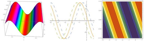
Figure 1.
The GOS graphs of in Equation (18) are presented via .

Figure 2.
The BOS graphs of in Equation (22) are expressed via .
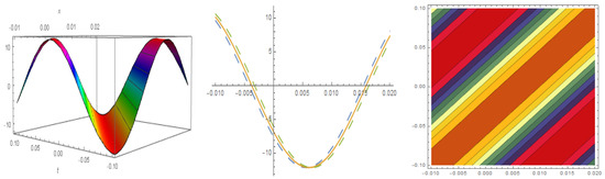
Figure 3.
The COS type-I graphs of in Equation (27) are presented via .
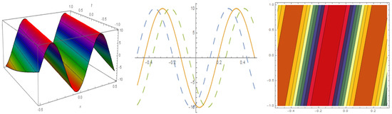
Figure 4.
The COS type-II graphs of in Equation (30) are plotted via .
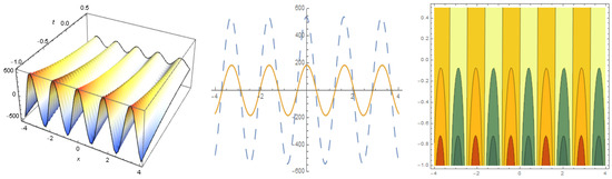
Figure 5.
The multiwave graphs of in Equation (42) are plotted with .
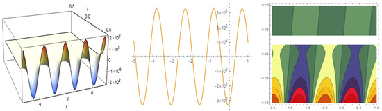
Figure 6.
The multiwave graphs of in Equation (42) are plotted with .
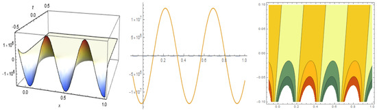
Figure 7.
The multiwave graphs of in Equation (42) are plotted with .
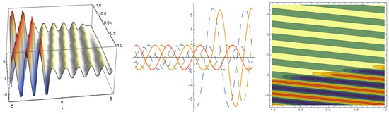
Figure 8.
The 3D, 2D and contour HB graphs of in Equation (42) are plotted with distinct parameters , respectively.
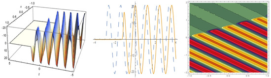
Figure 9.
The 3D, 2D and contour HB profiles of in Equation (42) are plotted with distinct parameters , respectively.
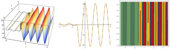
Figure 10.
The 3D, 2D and contour HB shapes of in Equation (42) are plotted with distinct parameters , respectively.
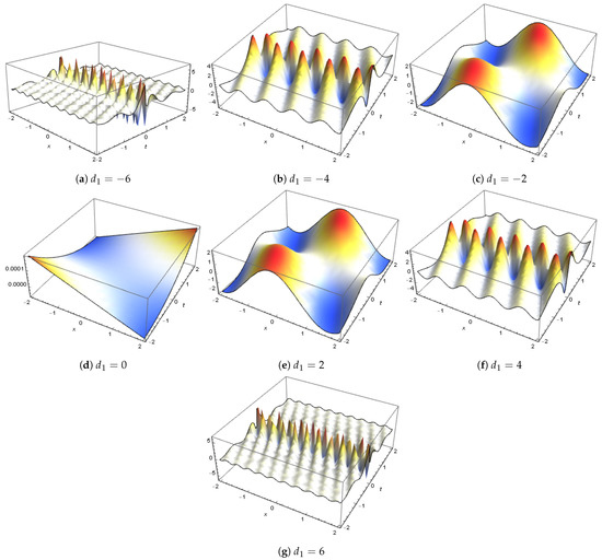
Figure 11.
The 3D M-shape soliton profiles for the solution in Equation (52) are constructed with .
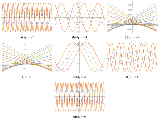
Figure 12.
The 2D M-shape soliton profiles for the solution in Equation (52) are constructed with .
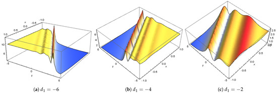
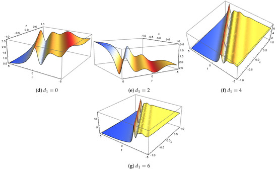
Figure 13.
One-kink interaction for M-shape soliton to Equation (57) via .
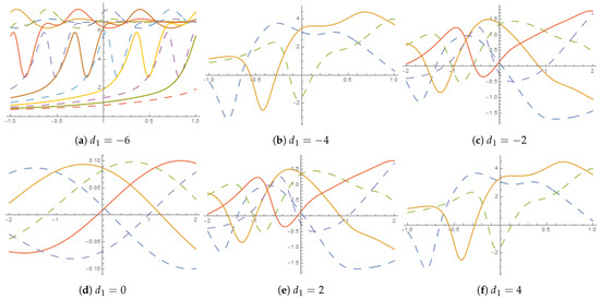
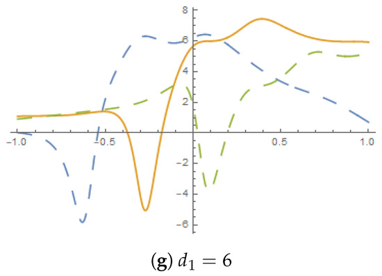
Figure 14.
The 2D profiles for Figure 13, respectively.
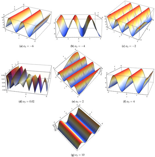
Figure 15.
The 3D M-shape soliton interaction profiles for the solution in Equation (60) are constructed with .
13. Conclusions
This article derived the grey and black optical solitons to the IP-NLSE with and dual power law nonlinearity via a complex envelope ansatz solution which arises in optical fibers and photovoltaic-photo-refractive materials. We thereafter applied the CLT to compute new forms of COS. Furthermore, the propagation of homoclinic breathers, multiwaves and M-shape solitons is analytically deliberated. All new analytical solutions are evaluated by ansatz functions techniques and transformation involving logarithmic functions. Multiwave solitons are successfully constructed by using the three-waves method. Two categories of interactions for M-shape solitons through exponential functions are successfully examined in Figure 13, Figure 14 and Figure 15.
Author Contributions
Methodology, S.T.R.R.; Formal analysis, S.A.M.A.; Supervision, A.R.S. All authors have read and agreed to the published version of the manuscript.
Funding
This research received no external funding.
Data Availability Statement
Not applicable.
Acknowledgments
The authors extend their appreciation to the Deanship for Research and Innovation, Ministry of Education in Saudi Arabia for funding this research work through the project number: IFP22UQU4290491DSR141.
Conflicts of Interest
The authors declare no conflict of interest.
References
- Baldelli, L.; Filippucci, R. Singular quasilinear critical Schrodinger equations in RN. Commun. Pure Appl. Anal. 2022, 21, 2561–2586. [Google Scholar] [CrossRef]
- Filippucci, R.; Pucci, P.; Souplet, P. A Liouville-type theorem in a half-space and its applications to the gradient blow-up behavior for superquadratic diffusive Hamilton-Jacobi equations. Comm. Partial. Differ. Equations 2020, 45, 321–349. [Google Scholar] [CrossRef]
- Seadawy, A.R.; Ahmed, S.; Rizvi, S.T.; Nazar, K. Applications for mixed Chen–Lee–Liu derivative nonlinear Schrödinger equation in water wave flumes and optical fibers. Optical Quantum Electron. 2023, 55, 34. [Google Scholar] [CrossRef]
- Seadawy, A.R.; Rizvi, S.T.; Ahmed, S.; Ahmad, A. Study of dissipative NLSE for dark and bright, multiwave, breather and M-shaped solitons along with some interactions in monochromatic waves. Opt. Quantum Electron. 2022, 54, 782. [Google Scholar] [CrossRef]
- Ahmed, S.; Seadawy, A.R.; Rizvi, S.T. Study of breathers, rogue waves and lump solutions for the nonlinear chains of atoms. Opt. Quantum Electron. 2022, 54, 320. [Google Scholar] [CrossRef]
- Ali, K.; Seadawy, A.R.; Ahmed, S.; Rizvi, S.T. Discussion on rational solutions for Nematicons in liquid crystals with Kerr Law. Chaos Solitons Fractals 2022, 160, 112218. [Google Scholar] [CrossRef]
- Seadawy, A.R.; Rizvi, S.T.; Ahmed, S. Weierstrass and Jacobi elliptic, bell and kink type, lumps, Ma and Kuznetsov breathers with rogue wave solutions to the dissipative nonlinear Schrödinger equation. Chaos Solitons Fractals 2022, 160, 112258. [Google Scholar] [CrossRef]
- Khater, A.H.; Obied Allah, M.H. Effects of rotation on Rayleigh-Taylor instabilities of an accelerating, compressible, perfectly conducting plane layer. Astrophys. Space Sci. 1984, 106, 245–255. [Google Scholar] [CrossRef]
- Helal, M.A. A Chebyshev spectral method for solving Korteweg–de Vries equation with hydrodynamical application. Chaos Solitons Fractals 2001, 12, 943–950. [Google Scholar] [CrossRef]
- Helal, M.A.; Mehanna, M.S. A comparative study between two different methods for solving the general Korteweg–de Vries Equation (GKdV). Chaos Solitons Fractals 2007, 33, 725–739. [Google Scholar] [CrossRef]
- Seadawy, A.R.; Cheemaa, N. Propagation of nonlinear complex waves for the coupled nonlinear Schrödinger Equations in two core optical fibers. Phys. A Stat. Mech. Appl. 2019, 529, 121330. [Google Scholar] [CrossRef]
- Ghaffar, A.; Ali, A.; Ahmed, S.; Akram, S.; Baleanu, D.; Nisar, K.S. A novel analytical technique to obtain the solitary solutions for nonlinear evolution equation of fractional order. Adv. Differ. Equ. 2020, 2020, 308. [Google Scholar] [CrossRef]
- Wazwaz, A.M. Higher dimensional nonlinear Schrödinger equations in anomalous dispersion and normal dispersive regimes: Bright and dark optical solitons. Optik 2020, 222, 165327. [Google Scholar] [CrossRef]
- Cheemaa, N.; Seadawy, A.R.; Chen, S. More general families of exact solitary wave solutions of the nonlinear Schrodinger equation with their applications in nonlinear optics. Eur. Phys. J. Plus 2018, 133, 547. [Google Scholar] [CrossRef]
- Arshad, M.; Seadawy, A.; Lu, D.; Wang, J. Travelling wave solutions of generalized coupled Zakharov–Kuznetsov and dispersive long wave equations. Results Phys. 2016, 6, 1136–1145. [Google Scholar] [CrossRef]
- Helal, M.A. Solitons, A Volume in the Encyclopedia of Complexity and Systems Science, 2nd ed.; Springer Science: Berlin, Germany, 2022. [Google Scholar]
- Seadawy, A.R. Stability analysis of traveling wave solutions for generalized coupled nonlinear KdV equations. Appl. Math. Inf. Sci. 2016, 10, 209–214. [Google Scholar] [CrossRef]
- Seadawy, A.R.; Iqbal, M.; Lu, D. Application of mathematical methods on the ion sound and Langmuir waves dynamical systems. Praman-J. Phys. 2019, 93, 10. [Google Scholar] [CrossRef]
- Liu, Y.; Li, B.; Wazwaz, A.M. Novel high-order breathers and rogue waves in the Boussinesq equation via determinants. Int. J. Mod. Phys. B 2020, 43, 3701–3715. [Google Scholar] [CrossRef]
- Shah, K.; Seadawy, A.R.; Arfan, M. Evaluation of one dimensional fuzzy fractional partial differential equations. Alex. Eng. J. 2020, 59, 3347–3353. [Google Scholar] [CrossRef]
- Wang, J.; Shehzad, K.; Seadawy, A.R. Muhammad Arshad and Farwa Asmat, Dynamic study of multi-peak solitons and other wave solutions of new coupled KdV and new coupled Zakharov–Kuznetsov systems with their stability. J. Taibah Univ. Sci. 2023, 17, 2163872. [Google Scholar] [CrossRef]
- Wazwaz, A.M.; Mehanna, M. Bright and dark optical solitons for a new (3+ 1)-dimensional nonlinear Schrödinger equation. Optik 2021, 241, 166985. [Google Scholar] [CrossRef]
- Triki, H.; Biswas, A.; Milovic, D.; Belic, M. Chirped femtosecond pulses in the higher-order nonlinear Schrödinger equation with non-Kerr nonlinear terms and cubic–quintic–septic nonlinearities. Opt. Commun. 2016, 366, 362–369. [Google Scholar] [CrossRef]
- Taghizadeh, N.; Mirzazadeh, M.; Farahrooz, F. Exact solutions of the nonlinear Schrödinger equation by the first integral method. J. Math. Anal. Appl. 2011, 374, 549–553. [Google Scholar] [CrossRef]
- Seadawy, A.R. The generalized nonlinear higher order of KdV equations from the higher order nonlinear Schrödinger equation and its solutions. Optik 2017, 139, 31–34. [Google Scholar] [CrossRef]
- Chen, J.; Luan, Z.; Zhou, Q.; Alzahrani, A.K.; Biswas, A.; Liu, W. Periodic soliton interactions for higher-order nonlinear Schrödinger equation in optical fibers. Nonlinear Dyn. 2020, 100, 2817–2821. [Google Scholar] [CrossRef]
- Savaissou, N.; Gambo, B.; Rezazadeh, H.; Bekir, A.; Doka, S.Y. Exact optical solitons to the perturbed nonlinear Schrödinger equation with dual-power law of nonlinearity. Opt. Quantum Electron. 2020, 52, 318. [Google Scholar] [CrossRef]
- Kudryashov, N.A. Almost general solution of the reduced higher-order nonlinear Schrödinger equation. Optik 2021, 230, 166347. [Google Scholar] [CrossRef]
- Kudryashov, N.A. Optical solitons of the resonant nonlinear Schrödinger equation with arbitrary index. Optik 2021, 235, 166626. [Google Scholar] [CrossRef]
- Ma, G.; Zhao, J.; Zhou, Q.; Biswas, A.; Liu, W. Soliton interaction control through dispersion and nonlinear effects for the fifth-order nonlinear Schrödinger equation. Nonlinear Dyn. 2021, 106, 2479–2484. [Google Scholar] [CrossRef]
- Wang, K.J.; Wang, G.D. Variational theory and new abundant solutions to the (1+ 2)-dimensional chiral nonlinear Schrödinger equation in optics. Phys. Lett. A 2021, 412, 127588. [Google Scholar] [CrossRef]
- Mo, Y.; Ling, L.; Zeng, D. Data-driven vector soliton solutions of coupled nonlinear Schrödinger equation using a deep learning algorithm. Phys. Lett. A 2022, 421, 127739. [Google Scholar] [CrossRef]
- Jiang, C.; Cui, J.; Qian, X.; Song, S. High-order linearly implicit structure-preserving exponential integrators for the nonlinear Schrödinger equation. J. Sci. Comput. 2022, 90, 66. [Google Scholar] [CrossRef]
- Weng, W.; Zhang, G.; Zhang, M.; Zhou, Z.; Yan, Z. Semi-rational vector rogon-soliton solutions and asymptotic analysis for any n-component nonlinear Schrödinger equation with mixed boundary conditions. Phys. D Nonlinear Phenom. 2022, 432, 133150. [Google Scholar] [CrossRef]
- Biswas, A.; Ekici, M.; Sonmezoglu, A.; Arshed, S.; Belic, M. Optical soliton perturbation with full nonlinearity by extended trial function method. Opt. Quantum Electron. 2017, 44, 125–138. [Google Scholar] [CrossRef]
- Ekici, M.; Sonmezoglu, A.; Zhou, Q.; Moshokoa, S.P.; Ullah, M.Z.; Arnous, A.H.; Belic, M. Analysis of optical solitons in nonlinear negative-indexed materials with anti-cubic nonlinearity. Opt. Quantum Electron. 2019, 53, 715. [Google Scholar] [CrossRef]
- Seadawy, A.R.; Rizvi, S.T.; Ashraf, M.A.; Younis, M.; Hanif, M. Rational solutions and their interactions with kink and periodic waves for a nonlinear dynamical phenomenon. Int. J. Mod. Phys. B 2021, 35, 2150236. [Google Scholar] [CrossRef]
- Manafian, J.; Mohammadi Ivatloo, B.; Abapour, M. Breather wave, periodic, and cross-kink solutions to the generalized Bogoyavlensky-Konopelchenko equation. Math. Methods Appl. Sci. 2020, 43, 1753–1774. [Google Scholar] [CrossRef]
- Alsallami, S.A.M.; Rizvi, S.T.R.; Seadawy, A.R. Study of Stochastic–Fractional Drinfel’d–Sokolov–Wilson Equation for M-Shaped Rational, Homoclinic Breather, Periodic and Kink-Cross Rational Solutions. Mathematics 2023, 11, 1504. [Google Scholar] [CrossRef]
- Aliyu, A.I.; Tchier, F.; Inc, M.; Yusuf, A.; Baleanu, D. Dynamics of optical solitons, multipliers and conservation laws to the nonlinear Schrödinger equation in (2+1)-dimensions with non-Kerr law nonlinearity. J. Mod. Opt. 2019, 1950, 1162–1174. [Google Scholar] [CrossRef]
- Ahmed, I.; Seadawy, A.R.; Lu, D. Kinky breathers, W-shaped and multi-peak solitons interaction in (2+1)-dimensional nonlinear Schrödinger equation with Kerr law of nonlinearity. Eur. Phys. J. Plus 2019, 134, 1–10. [Google Scholar] [CrossRef]
- Ahmed, I.; ASeadawy, R.; Lu, D. M-shaped rational solitons and their interaction with kink waves in the Fokas–Lenells equation. Phys. Scr. 2019, 94, 055205. [Google Scholar] [CrossRef]


Disclaimer/Publisher’s Note: The statements, opinions and data contained in all publications are solely those of the individual author(s) and contributor(s) and not of MDPI and/or the editor(s). MDPI and/or the editor(s) disclaim responsibility for any injury to people or property resulting from any ideas, methods, instructions or products referred to in the content. |
© 2023 by the authors. Licensee MDPI, Basel, Switzerland. This article is an open access article distributed under the terms and conditions of the Creative Commons Attribution (CC BY) license (https://creativecommons.org/licenses/by/4.0/).